Advancing density waves and phase transitions in a
velocity dependent randomization traffic cellular automaton

Abstract

Within the class of stochastic cellular automata models of traffic flows, we look at the velocity dependent randomization variant (VDR-TCA) whose parameters take on a specific set of extreme values. These initial conditions lead us to the discovery of the emergence of four distinct phases. Studying the transitions between these phases, allows us to establish a rigorous classification based on their tempo-spatial behavioral characteristics. As a result from the system’s complex dynamics, its flow-density relation exhibits a non-concave region in which forward propagating density waves are encountered. All four phases furthermore share the common property that moving vehicles can never increase their speed once the system has settled into an equilibrium.

I Introduction

In the field of traffic flow modeling, microscopic traffic simulation has always been regarded as a time consuming, complex process involving detailed models that describe the behavior of individual vehicles. Approximately a decade ago, however, new microscopic models were being developed, based on the cellular automata programming paradigm from statistical physics. The main advantage was an efficient and fast performance when used in computer simulations, due to their rather low accuracy on a microscopic scale. These so-called traffic cellular automata (TCA) are discrete in nature, in the sense that time advances with discrete steps and space is coarse-grained (allowing for high-speed simulations, especially when they are performed on a platform for parallel computation) Maerivoet and Moor (2003).

The seminal work done by Nagel and Schreckenberg in the construction of their stochastic traffic cellular automaton (i.e., the STCA) Nagel and Schreckenberg (1992), led to a global adoptation of the TCA modeling scheme. In order to generate traffic jams, their model needs some kind of fluctuations, which are introduced by means of a noise parameter. But one of the artefacts associated with this STCA model, is that it gives rise to (many) unstable traffic jams Nagel (1994). A possible approach to achieve stable traffic jams, is to reduce the outflow from such jams, which can be accomplished by implementing so-called slow-to-start behavior. The name is derived from the fact that vehicles exiting jam fronts are obliged to wait a small amount of time. One of these implementations, is the approach initially followed by Takayasu and Takayasu Takayasu and Takayasu (1993). They made the stochastic noise dependent on the distance between two consecutive vehicles. Another implementation is based on making this noise parameter dependent on the velocity of a vehicle, leading to the development of the velocity dependent randomization (VDR) TCA. This TCA model moreover exhibits metastability and hysteresis phenomena Barlović et al. (1998).

In this context, our paper addresses the VDR-TCA slow-to-start model whose parameters take on a specific set of extreme values. Even though this bears little direct relevance for the understanding of traffic flows, it will lead to an induced ‘anomalous’ behavior and complex system dynamics, resulting in four distinct emergent phases. We study these on the basis of the system’s relation between density and flow (i.e., the fundamental diagram) which exhibits a non-concave region where, in contrast to the properties of congested traffic flow, density waves are propagated forwards. We furthermore investigate the system’s tempo-spatial evolution in each of these four phases, and consider an order parameter that allows us to track the transitions between them.

Although some related studies exist (e.g., Awazu (1999); Grabolus (2001); Gray and Griffeath (2001); Leveque (2001); Nishinari et al. (2003); Zhang (2003)), the special behavior discussed in this paper has not been reported as such, as most previously done research is largely devoted to empirical and analytical discussions about these TCA models, operating under normal conditions. To strengthen our claims, we compare our results with the existing literature at the end of this paper.

In section II, we briefly describe the concept of a traffic cellular automaton and the experimental setup used when performing the simulations. The selected VDR-TCA model is presented in section III, as well as an account of some behavioral characteristics under normal operating conditions. The results of our various experiments with more complex system dynamics are subsequently presented and extensively discussed in section IV, after which the paper concludes with a comparison with existing literature in section V and a summary in section VI.

II Experimental setup

In this section, we introduce the operational characteristics of a standard single-lane traffic cellular automaton model. To avoid confusion with some of the notations in existing literature, we explicitly state our definitions.

II.1 Geometrical description

Let us describe the operation of a single-lane traffic cellular automaton as depicted in Fig. 1. We assume $N$ vehicles are driving on a circular lattice containing $K$ cells, i.e., periodic boundary conditions (each cell can be occupied by at most one vehicle at a time). Time and space are discretized, with $\Delta T=1$ s and $\Delta X=7.5$ m, leading to a velocity discretization of $\Delta V=27$ km/h. Furthermore, the velocity $v_{i}$ of a vehicle $i$ is constrained to an integer in the range $\{0,\ldots,v_{\mbox{max}}\}$, with $v_{\mbox{max}}$ typically 5 cells/s (corresponding to 135 km/h).

\psfrag{t}{\footnotesize{$t$}}\psfrag{t+1}{\footnotesize{$t+1$}}\psfrag{i}{\footnotesize{$i$}}\psfrag{j}{\footnotesize{$j$}}\psfrag{deltat}{\footnotesize{$\Delta T$}}\psfrag{deltax}{\footnotesize{$\Delta X$}}\psfrag{gsi}{\footnotesize{$g_{s_{i}}$}}\includegraphics[width=233.3125pt]{Figures/TXDiagrams/general/tca-basics.eps}

Figure 1: Schematic diagram of the operation of a single-lane traffic cellular automaton (TCA); here, the time axis is oriented downwards, the space axis extends to the right. The TCA’s configuration is shown for two consecutive time steps $t$ and $t+1$, during which two vehicles $i$ and $j$ propagate through the lattice. Without loss of generality, we denote the number of empty cells in front of vehicle $i$ as its space gap $g_{s_{i}}$.

Each vehicle $i$ has a space headway $h_{s_{i}}$ and a time headway $h_{t_{i}}$, defined as follows:

$$h_{s_{i}} = L_{i}+g_{s_{i}},$$ (1)

$$h_{t_{i}} = \rho_{i}+g_{t_{i}}.$$ (2)

In these definitions, $g_{s_{i}}$ and $g_{t_{i}}$ denote the space and time gaps respectively; $L_{i}$ is the length of a vehicle and $\rho_{i}$ is the occupancy time of the vehicle (i.e., the time it ‘spends’ in one cell). Note that in a traffic cellular automaton the space headway of a vehicle is always an integer number, representing a multiple of the spatial discretisation $\Delta X$ in real world measurement units. So in a jam, it is taken to be equal to the space the vehicle occupies, i.e., $h_{s_{i}}=$ 1 cell.

Local interactions between individual vehicles in a traffic stream are modeled by means of a rule set that reflects the car-following behavior of a cellular automaton evolving in time and space. In this paper, we assume that all vehicles have the same physical characteristics (i.e., homogeneous traffic). The system’s state is changed through synchronous position updates of all the vehicles, based on a rule set that reflects the car-following behavior.

Most rule sets of TCA models do not use the space headway $h_{s_{i}}$ or the space gap $g_{s_{i}}$, but are instead based on the number of empty cells $d_{i}$ in front of a vehicle $i$. Keeping equation (1) in mind, we therefore adopt the following convention from this moment on: we assume that, without loss of generality, for a vehicle $i$ its length $L_{i}=1$ cell. This means that when the vehicle is residing in a compact jam, its space headway $h_{s_{i}}=1$ cell and its space gap is consequently $g_{s_{i}}=0$ cells (i.e., equivalent to the number of empty cells $d_{i}$ in front of the vehicle). This abstraction gives us a rigorous justification to formulate the TCA’s update rules more intuitively using space gaps.

II.2 Performing measurements

In order to characterize the behavior of a TCA model, we perform global measurements on the system’s lattice. These measurements are expressed as macroscopic quantities, defining the global density $k$, the space mean speed $\overline{v}_{s}$, and the flow $q$ as:

$$k = \frac{N}{K},$$ (3)

$$\overline{v}_{s} = \frac{1}{N}\sum_{i=1}^{N}{v_{i}},$$ (4)

$$q = k\overline{v}_{s},$$ (5)

with $N$ the number of vehicles in the system and $K$ the number of cells in the lattice. The above measurements are calculated every time step, and they should be averaged over a large measurement period $T_{\mbox{sim}}$ in order to allow the system to settle into an equilibrium.

Correlation plots of these aggregate quantities lead to time-independent graphs conventionally called ‘fundamental diagrams’ (e.g., Fig. 3). An important remark is that is that these diagrams are actually only valid under stationary traffic conditions and for homogeneous traffic, which is almost never the case. As such, real-life traffic does not ‘lie’ on this curve because it represents the ‘average behavior’ of the vehicles in a traffic stream. And although we should more correctly refer to our measurements as points in a certain phase space (e.g., the ($k$,$q$) phase space), we will still use the terminology of ‘fundamental diagram’ in the remainder of this paper when we are in fact referring to this phase space.

Note that we also can calculate these macroscopic quantities as local averages (i.e., local in time and space), but these lead to the same results as for large systems and measurements periods Nagel (1995).

The previous global macroscopic measurements (density, average speed, and flow) from equations (3), (4), and (5), can be related to the microscopic equations (1) and (2) as follows:

$$k \propto \overline{h}_{s}^{-1},$$ (6)

$$q \propto \overline{h}_{t}^{-1},$$ (7)

with $\overline{h}_{s}$ and $\overline{h}_{t}$ the average space and time headway respectively. Note that with respect to the time gaps and time headways, we will work in the remainder of this paper with the median instead of the arithmetic mean because the former gives more robust results when $h_{t_{i}},g_{t_{i}}\rightarrow+\infty$ for a vehicle $i$.

All the fundamental diagrams in this paper, were calculated using systems of $10^{3}$ cells. The first $10^{3}$ s of each simulation were discarded in order to let initial transients die out; the system was then updated for $T_{\mbox{sim}}=10^{4}$ s.

For a deeper insight into the behavior of the space mean speed $\overline{v}_{s}$, the average space gap $\overline{g}_{s}$, and the median time gap $\overline{g}_{t}$, detailed histograms showing their distributions are provided. These are interesting because in the existing literature (e.g., Chowdhury et al. (1998); Schadschneider (2000); Helbing (2001)) these distributions are only considered at several distinct global densities, whereas we show them for all densities. Each of our histograms is constructed by varying the global density $k$ between 0.0 and 1.0, calculating the average speed, the average space gap and the median time gap for each simulation run. A simulation run consists of $5\times 10^{4}$ s (with a transient period of 500 s) on systems of 300 cells, varying the density in 150 steps. Note that a larger size of the system’s lattice, has no significant effects on the results, except for an increase of the variance.

All the experiments were carried out with our Java software ”Traffic Cellular Automata”, which can be found at http://smtca.dyns.cx Maerivoet (2004).

III Velocity dependent randomization

In this section, the rule set of the VDR-TCA model is explained, followed by a an overview of the model’s tempo-spatial behavior and its related macroscopic quantities (i.e., the fundamental diagrams and the distributions of the speeds and the space and time gaps) under normal conditions.

III.1 The VDR-TCA’s rule set

As indicated before, we focus our research on the VDR-TCA model for the implementation of the car-following behavior. The following equations (based on Barlović et al. (1998)) form its rule set; the rules are applied consecutively to all vehicles in parallel (i.e., synchronous updates):

R1:

determine stochastic noise

$$\left\{\begin{array}[]{lcl}v_{i}(t-1)=0&\Longrightarrow&p^{\prime}\leftarrow p_{0},\\ v_{i}(t-1)>0&\Longrightarrow&p^{\prime}\leftarrow p,\\ \end{array}\right.$$ (8)

R2:

acceleration and braking

$$v_{i}(t)\leftarrow\min\{v_{i}(t-1)+1,g_{s_{i}}(t-1),v_{\mbox{max}}\},$$ (9)

R3:

randomization

$$\xi_{i}(t)<p^{\prime}\Longrightarrow v_{i}(t)\leftarrow\max\{0,v_{i}(t)-1\},$$ (10)

R4:

vehicle movement

$$x_{i}(t)\leftarrow x_{i}(t-1)+v_{i}(t).$$ (11)

In the above equations, $v_{i}(t)$ is the speed of vehicle $i$ at time $t$ (i.e., in the current updated configuration of the system), $v_{\mbox{max}}$ is the maximum allowed speed, $g_{s_{i}}$ denotes the space gap of vehicle $i$ and $x_{i}\in\{1,\ldots,K\}$ an integer number denoting its position in the lattice. In the third rule, equation (10), $\xi_{i}(t)\in[0,1[$ denotes a uniform random number (specifically drawn for vehicle $i$ at time $t$) and $p^{\prime}$ is the stochastic noise parameter, dependent on the vehicle’s speed ($p_{0}$ is called the slow-to-start probability and $p$ the slowdown probability, with $p_{0},p\in[0,1]$).

In a nutshell, rule R1, equation (8), determines the correct velocity dependent randomization. Note that we only consider the case with two different noise parameters (i.e., $p_{0}$ and $p$), ignoring the more general case where we have a noise parameter for each possible speed (i.e., $p_{0}$, …, $p_{v_{\mbox{max}}}$). Rule R2, equation (9), states that a vehicle tries to increase its speed at each time step, as long as it hasn’t reached its maximal speed and it has enough space headway. It also states that when a vehicle hasn’t enough space headway, it abruptly adapts its speed in order to prevent a collision with the leading vehicle (the model thus exhibits an infinite braking capability). The randomization parameter determined in equation (8), is now used in rule R3, equation (10), to introduce a stochastic component in the system: a vehicle will randomly slow down with probability $p^{\prime}$. The last rule R4, equation (11), isn’t actually a ‘real’ rule; it just allows the vehicles to advance in the system.

III.2 Normal behavioral characteristics

Depending on their speed, vehicles are subject to different randomizations: typical metastable behavior results when $p_{0}\gg p$, meaning that stopped vehicles have to wait longer before they can continue their journey (i.e, they are ‘slow-to-start’). This has the effect of a reduced outflow from a jam, so that, in a closed system, this leads to an equilibrium and the formation of a compact jam. For such a typical situation (e.g., $p_{0}=0.5$ and $p=0.01$), the tempo-spatial evolution is depicted in Fig. 2; each vehicle is represented by a single colored dot; as time advances, vehicles move to the upper right corner, whereas congestion waves move to the lower right corner, i.e., backwards in space (note that the orientation of the axes is different than the one Fig. 1). We can see an initially homogeneous traffic pattern (one metastable phase) breaking down and kicking the system into a phase separated state (two phases: free-flowing traffic and a compact jam).

\psfrag{580s}{\footnotesize{Time (580~{}s)}}\psfrag{300cells}{\footnotesize{Space (300~{}cells)}}\includegraphics[width=244.69386pt]{Figures/TXDiagrams/vdrtca/tx-diagram-vdrtca-k0.1667-sp0.01-s2sp0.5.eps}

Figure 2: A typical time-space diagram of the VDR-TCA model. The shown lattice contains 300 cells (corresponding to 2.25 km), the visible time horizon is 580 seconds. The slow-to-start probability $p_{0}$ was set to 0.5, the slowdown probability $p$ to 0.01, and the global density equal to the system’s critical density. We can see a phase separation taking place, forming a persistent compact jam surrounded by free-flowing traffic. The significant decrease of the density in the regions outside the jam results from the jam’s reduced outflow.

Studying the ($k$,$q$) fundamental diagram in Fig. 3, gives us another view of this phase transition. The free-flow branch was obtained by initially distributing the vehicles homogeneously over the system’s lattice, whereas they were placed in a compact superjam (i.e., all vehicles are ‘bunched up’ behind each other) in order to obtain the congested branch. We can see a ‘capacity drop’ taking place at the critical density, where traffic in its vicinity behaves in a metastable manner. This metastability is characterized by the fact that sufficiently large disturbances of the fragile equilibrium can cause the flow to undergo a sudden decrease, corresponding to a first-order phase transition in statistical physics. The state of very high flow is then destroyed and the system settles into a phase separated state with a large megajam and a free-flow zone Barlović et al. (1998); Chowdhury et al. (2000). The large jam will persist as long as the density is not significantly lowered, meaning that recovery of traffic from congestion thus shows a hysteresis phenomenon Barlović et al. (1999).

\psfrag{Global density k}{\footnotesize{Global density $k$}}\psfrag{Flow q [vehicles/hour]}{\footnotesize{Flow $q$ [vehicles/h]}}\psfrag{Homogeneous state}[l][l]{\footnotesize{Homogeneous state}}\psfrag{Superjam}[l][l]{\footnotesize{Superjam}}\includegraphics[width=244.69386pt]{Figures/FundamentalDiagrams/vdrtca/fundamental-diagrams-k-q-vdrtca-metastability-c10000-tp1000-sp10000-vmax5-sp0.01-s2sp0.5.eps}

Figure 3: Typical ($k$,$q$) fundamental diagram of the VDR-TCA (with the slow-to-start probability $p_{0}$ set to 0.5 and the slowdown probability $p$ set to 0.01). The typical ‘reversed $\lambda$’ shape is obtained by going from the free-flowing to the congested traffic regime and vice versa, resulting in hysteretic behavior (i.e., the directions of the arrows); in the first case, traffic encounters a capacity drop, whereas in the second case, the recovery results in a lower value for the flow.

Considering the non-stochastic CA-184 (i.e., Wolfram’s rule 184 with $v_{\mbox{max}}>1$ Wolfram (2002)), we can calculate the critical density (where the transition between the free-flowing and congested phases occurs) as Schadschneider (2002):

$$k_{c}=\frac{1}{L+v_{\mbox{max}}}.$$ (12)

Setting $v_{\mbox{max}}=5$ cells/s (this equals $5\times 7.5\times 3.6=135$ km/h), we correspondingly get $k_{c}=(1+5)^{-1}=0.1\overline{6}$. Note that this number is dimensionless because $k_{c}$ represents the fraction of the maximum density, i.e., the jam density $k_{j}=(\Delta X)^{-1}=133.\overline{3}$ vehicles/km. Converting the value of the critical density to real world measurement units, we obtain $k_{c}=0.1\overline{6}\times 133.\overline{3}=22.\overline{2}$ vehicles/km. The associated capacity flow $q_{\mbox{cap}}=k_{c}\cdot\overline{v}_{\mbox{max}}=135\times 22.\overline{2}=3000$ vehicles/h. Note that this number is an overestimate for our system, as an exact formula expressing the capacity flow $q_{\mbox{cap}}$ in function of the maximum speed $v_{\mbox{max}}$, the slowdown probability $p$, and the lattice size $K$, has not yet been determined Maerivoet et al. (2003). If we perform a linear regression on the congested branch of Fig. 3, we get the speed of the backward propagating congestion waves, which is $\approx-13.5$ km/h, close to the empirical value of -15 km/h found in real-life traffic Helbing (2001).

\psfrag{Global density k}{\footnotesize{Global density $k$}}\psfrag{Speed v [cells/s]}{\footnotesize{Speed $v$ [cells/s]}}\psfrag{(A)}{\footnotesize{($A$)}}\psfrag{(B)}{\footnotesize{($B$)}}\psfrag{Histogram class [speed v in cells/s]}{}\psfrag{Histogram class probability}{\footnotesize{Class probability}}\includegraphics[width=233.3125pt]{Figures/Histograms/vdrtca/histogram-speed-vdrtca-c300-s150-tp500-sp50000-vmax5-sp0.01-s2sp0.5.eps}

\psfrag{Global density k}{\footnotesize{Global density $k$}}\psfrag{Speed v [cells/s]}{\footnotesize{Speed $v$ [cells/s]}}\psfrag{(A)}{\footnotesize{($A$)}}\psfrag{(B)}{\footnotesize{($B$)}}\psfrag{Histogram class [speed v in cells/s]}{}\psfrag{Histogram class probability}{\footnotesize{Class probability}}\includegraphics[width=233.3125pt,height=85.35826pt]{Figures/Histograms/vdrtca/histogram-cross-section-speed-vdrtca-c300-s150-tp500-sp50000-vmax5-sp0.01-s2sp0.5-d0.1325.eps} \psfrag{Global density k}{\footnotesize{Global density $k$}}\psfrag{Speed v [cells/s]}{\footnotesize{Speed $v$ [cells/s]}}\psfrag{(A)}{\footnotesize{($A$)}}\psfrag{(B)}{\footnotesize{($B$)}}\psfrag{Histogram class [speed v in cells/s]}{}\psfrag{Histogram class probability}{\footnotesize{Class probability}}\includegraphics[width=233.3125pt,height=85.35826pt]{Figures/Histograms/vdrtca/histogram-cross-section-speed-vdrtca-c300-s150-tp500-sp50000-vmax5-sp0.01-s2sp0.5-d0.4000.eps} Histogram class [speed $v$ in cells/s]

Figure 4: The distribution of the vehicles’ speeds $v$, as a function of the global density $k$ in the VDR-TCA (with $p_{0}=0.5$ and $p=0.01$). In the contourplot to the left, the thick solid line denotes the space mean speed, whereas the thin solid line shows its standard deviation. The grey regions denote the probability densities. The histograms ($A$) and ($B$) to the right, show two cross sections made in the left contourplot at $k=0.1325$ and $k=0.4000$ respectively: for example, in ($A$), the high concentration of probability mass at the histogram class $v=$ 5 cells/s corresponds to the dark region in the upper left corner of the contourplot.

If we look at the distribution of the vehicles’ speeds, we get the histogram in Fig. 4. Here we can clearly see the distinction between the free-flowing and the congested phase: the space mean speed remains constant at a high value, then encounters a sharp transition (i.e., the capacity drop), resulting in a steady declination as the global density increases. Note that as the critical density is encountered, the standard deviation jumps steeply; this means that vehicles’ speeds fluctuate wildly at the transition point (because they are entering and exiting the congestion waves). Once the compact jam is formed, the dominating speed quickly becomes zero (because vehicles are standing still inside the jam). Although most of the weight is attributed to this zero-speed, there is a non-negligible maximum speed present for intermediate densities. If the global density is increased further towards the jam density, this maximum speed disappears and the system settles into a state in which all vehicles either have speed zero or one (i.e., systemwide stop-and-go traffic).

Considering the distribution of the vehicles’ space gaps, we get Fig. 5; because of their tight coupling in the VDR-TCA’s rule set, the courses of both the space mean speed and the average space gaps are similar. Although the space gaps are rather large for low densities, at the critical density $k_{c}$ they leave a small cluster around an optimal value. This value can be calculated using equations (1), (6), and (12) (noting that $\overline{L}=L=1$ because we are dealing with homogeneous traffic):

$$\overline{g}_{s}=\overline{h}_{s}-\overline{L}=\frac{1}{k_{c}}-L,$$ (13)

resulting in $\lceil\overline{g}_{s}\rceil=\lceil 0.1669^{-1}-1\rceil=\lceil 4.99\rceil=5$ cells. This corresponds to the necessary minimal space gap in order to travel at the maximum speed, avoiding a collision with the leader. An important observation is that no recorded space gaps exist between this cluster of five cells and the space gaps of zero cells inside the compact jam. This means that there is a distinct phase separation taking place once beyond the critical density: vehicles are either completely in the free-flowing regime, or they are in the compact jam.

\psfrag{Global density k}{\footnotesize{Global density $k$}}\psfrag{Space gap gs [cells]}{\footnotesize{Space gap $g_{s}$ [cells]}}\psfrag{>= 10}{\footnotesize{$\geq$~{}10}}\includegraphics[width=244.69386pt]{Figures/Histograms/vdrtca/histogram-spacegap-vdrtca-c300-s150-tp500-sp50000-vmax5-sp0.01-s2sp0.5.eps}

Figure 5: The distribution of the vehicles’ space gaps $g_{s}$, as a function of the global density $k$ in the VDR-TCA (with $p_{0}=0.5$ and $p=0.01$). The thick solid line denotes the average of all the vehicles’ space gaps, whereas the thin solid line shows its standard deviation. The grey regions denote the probability densities.

Figure 6 shows the distribution of the vehicles’ time gaps: when traffic is in the free-flowing regime, time gaps are high, but finite. As the critical density is approached, the median time gap first decreases (because the vehicles’ speeds remain the same but their space gaps decrease). Once beyond the critical density, it increases towards infinity because vehicles come to a full stop inside the compact jam. Just as with the space gaps, we can also observe a small cluster around an optimal value. This optimal time gap, is the time needed to travel the distance formed by the optimal space gap, at the maximum speed. This means that $\overline{g}_{t}=\overline{g}_{s}\div v_{\mbox{max}}=1$ s. Because the previous train of thought is only exactly valid for the non-stochastic CA-184 and the VDR-TCA incorporates stochastic noise, the median optimal time gap lies somewhat above the previously calculated value ($\overline{g}_{t}\approx 1.2$ s).

\psfrag{Global density k}{\footnotesize{Global density $k$}}\psfrag{Time gap gt [seconds]}{\footnotesize{Time gap $g_{t}$ [seconds]}}\psfrag{+INF}{\footnotesize{$+\infty$}}\includegraphics[width=244.69386pt]{Figures/Histograms/vdrtca/histogram-timegap-vdrtca-c300-s150-tp500-sp50000-vmax5-sp0.01-s2sp0.5.eps}

Figure 6: The distribution of the vehicles’ time gaps $g_{t}$, as a function of the global density $k$ in the VDR-TCA (with $p_{0}=0.5$ and $p=0.01$). The thick solid line denotes the median of all the vehicles’ time gaps. The grey regions denote the probability densities.

IV More complex system dynamics

Most of the previous research dealt with the study of the behavioral characteristics of the VDR-TCA model operating under normal conditions. We now turn our attention to the specific case in which the model’s parameters take on extreme values $p_{0}\ll p$, more specifically considering the limiting case where $p_{0}=0.0$ and $p=1.0$.

We will first look at the change in tempo-spatial behavior when $p$ is increased towards 1.0, at which point a peculiar behavior is established in the system. We study the qualitative effects that the VDR-TCA’s rule set has on individual vehicles, and discuss shortly the prevailing initial conditions. This is followed by a quantitative analysis using the ($k$,$q$) and ($k$,$\overline{v}_{s}$) fundamental diagrams. The former diagram leads us to the discovery of four distinct phases, having a non-concave region with forward propagating density waves. More elaborate explanations are given based on the histograms of the space mean speed, the average space gap, and the median time gap. This is followed by a detailed analysis of the observations of the tempo-spatial behavior of the system in each of the four different phases (i.e., traffic regimes). The section concludes with a short discussion on the effects of different maximal speeds, after which we adopt the use of an order parameter that is able to track the phase transitions between the different traffic regimes.

IV.1 Increasing the stochastic noise $p$

Let us first consider the case in which $p_{0}=0.0$ and where we vary $p$ between 0.0 and 1.0. Figure 7 shows a time-space diagram where we simulated a system consisting of 300 cells. As time advances (over a period of 580 s), the slowdown probability $p$ is steadily increased from 0.0 to 1.0 (the global density $k$ was set to 0.1667 which is slightly below the critical density for a system with stochastic noise).

\psfrag{580s}{\footnotesize{Time (580~{}s) with $p\in[0\rightarrow 1]$}}\psfrag{300cells}{\footnotesize{Space (300~{}cells)}}\includegraphics[width=244.69386pt]{Figures/TXDiagrams/vdrtca/tx-diagram-vdrtca-k0.1667-sp0.0-1.0-s2sp0.0.eps}

Figure 7: A time-space diagram showing a system with a lattice of 300 cells (corresponding to 2.25 km); the visible time horizon is 580 seconds. As time advances, the slowdown probability $p$ varies between 0.0 and 1.0 (the slow-to-start probability $p_{0}$ was fixed at 0.0). The system’s global density $k$ is 0.1667.

When $p$ is very low, vehicles can keep driving in the free-flowing regime. As $p$ is increased, small unstable jams occur. Increasing $p$ even further, leads to even more pronounced jams. An important observation is that the propagation speed of these backward moving congestion waves increases; when $p$ reaches approximately 0.5, their speed equals 0, meaning that jams stay fixed at a position. Note that as these jams are unstable, they can be created or dissolved at arbitrary locations. Finally, as $p$ tends to 1.0, we can see the emergence of forward propagating congestion waves; ‘density’ is now being carried in the direction of the traffic flow. These forward propagating waves form ‘moving blockades’ that trap vehicles, which in turn leads to tightly packed clusters of vehicles that move steadily (but at a much slower pace than in the free-flowing regime). Note that this ‘clustering’ behavior is different from platooning, which typically occurs when vehicles are driving close to each other at relatively high speeds Lárraga et al. (2004). In our case, the clusters of vehicles advance more slowly.

IV.2 Qualitative effects of the rule set

From now on, we only consider the limiting case where $p_{0}=0.0$ and $p=1.0$. Let us now study the influence of the VDR-TCA’s rule set on an individual vehicle $i$. Assuming $v_{i}\in\{0,\ldots,v_{\mbox{max}}\}$, the rules described in section III.1 lead to the following four general cases:

• Case (1) with $v_{i}(t-1)=0$ and $g_{s_{i}}(t-1)=0$

  In this case, the vehicle is residing inside a jam and rule R2 (acceleration and braking) plays a dominant part: the vehicle’s speed $v_{i}(t)$ remains 0.
  

• Case (2) with $v_{i}(t-1)=0$ and $g_{s_{i}}(t-1)>0$

  This situation may arise when, for example, a vehicle is at a jam’s front. According to rule R1, the stochastic noise parameter $p^{\prime}$ becomes 0.0. Rule R2 then results in an updated speed $v_{i}(t)=\min\{1,g_{s_{i}}(t-1)\}=1$. Because there is no stochastic noise present in this case, rule R3 does not apply and the vehicle always advances one cell.
  

• Case (3) with $v_{i}(t-1)>0$ and $g_{s_{i}}(t-1)=0$

  Because there is no space in front of the vehicle, it has to brake in order to avoid a collision. Rule R2 consequently abruptly decreases the vehicle’s speed $v_{i}(t)$ to 0, as the vehicle needs to stop.
  

• Case (4) with $v_{i}(t-1)>0$ and $g_{s_{i}}(t-1)>0$

  This case deserves special attention, as there are now two discriminating possibilities:
  

  • Case (4a) with $v_{i}(t-1)<g_{s_{i}}(t-1)$

    According to rule R1, the stochastic noise $p^{\prime}$ becomes 1.0. Because the vehicle’s speed is strictly less than its space gap, rule R2 becomes $v_{i}(t)\leftarrow\min\{v_{i}(t-1)+1,v_{\mbox{max}}\}$. Finally, rule R3 is applied which always reduces the speed calculated in rule R2 (constrained to 0). In order to understand what is happening, consider the speeds $v_{i}(t-1)$ and $v_{i}(t)$ in the following table:

    $v_{i}(t-1)$		$v_{i}(t)$
    $v_{\mbox{max}}$	$\longrightarrow$	$v_{\mbox{max}}$ - 1
    $v_{\mbox{max}}$ - 1	$\longrightarrow$	$v_{\mbox{max}}$ - 1
    $v_{\mbox{max}}$ - 2	$\longrightarrow$	$v_{\mbox{max}}$ - 2
    ⋮		⋮
    2	$\longrightarrow$	2
    1	$\longrightarrow$	1

    We can clearly see that the maximum speed a vehicle can travel at, is constrained by $v_{\mbox{max}}$ - 1, which corresponds to $v_{\mbox{max}}-p^{\prime}$ Schreckenberg et al. (2001). From the table it follows that all vehicles traveling at $v_{i}<v_{\mbox{max}}$ can neither accelerate nor decelerate: the vehicles’ current speed is kept.
    

  • Case (4b) with $v_{i}(t-1)\geq g_{s_{i}}(t-1)$

    Just as in the previous case (4a), the stochastic noise $p^{\prime}$ becomes 1.0. Rule R2 now changes to $v_{i}(t)\leftarrow g_{s_{i}}(t-1)$. Because rule R3 is always applied, this results in $v_{i}(t)$ actually becoming $g_{s_{i}}(t-1)-1$ instead of just $g_{s_{i}}(t-1)$. So a vehicle always slows down too much (as opposed to solely avoiding a collision with its leader).

Conclusion: considering the previously discussed four general cases, the most striking feature is that, according to case (4a), in a VDR-TCA model with $p_{0}=0.0$ and $p=1.0$, a moving vehicle can never increase its speed, i.e., $v_{i}(t)\leq v_{i}(t-1)$.

IV.3 Effects of the initial conditions

As already mentioned, in this paper we study the limiting case where $p_{0}=0.0$ and $p=1.0$. This case is special, in the sense that the system’s behavior for light densities is extremely dependent on the initial conditions.

If we calculate the flow $q$ associated with each global density $k$ in the range $[0,\frac{1}{3}]$, we obtain Fig. 8. Here we show three curves for $v_{\mbox{max}}\in\{3,4,5\}$ where the system was initialized by distributing the vehicles homogeneously over the system’s lattice. A fourth curve is also shown, corresponding to $v_{\mbox{max}}=5$ where, as opposed to the previous initialization scheme, the system was initialized by distributing the vehicles randomly over the system’s lattice.

After the system has settled into an equilibrium, the resulting flow is limited by the fact that the maximum speed of a vehicle in the system is always equal to $v_{\mbox{max}}-1$. As proven in section IV.2, vehicles can never accelerate, which means that the slowest car in the system determines the maximum possible flow. Therefore, if the system (with $v_{\mbox{max}}=5$ cells/s) is initialized with a homogeneous distribution of the vehicles, then all of them will travel at $v_{\mbox{max}}-1=4$ cells/s (i.e., the upper branch in Fig. 8). If however, the system is initialized randomly, this has the effect that some vehicles are spaced more closely to each other. As a direct consequence of this, all vehicles will now travel at $v_{\mbox{max}}^{\prime}-1$ cells/s with $v_{\mbox{max}}^{\prime}$ the speed of the slowest vehicle in the system. In the extreme case, a single vehicle traveling at $v_{i}=1$ cell/s will cause all other vehicles to slow down to this speed, resulting in the lower branch in Fig. 8.

\psfrag{Global density k}{\footnotesize{Global density $k$}}\psfrag{Flow q [vehicles/hour]}{\footnotesize{Flow $q$ [vehicles/h]}}\psfrag{vMax = 5 (homogeneous)}[l][l]{\footnotesize{$v_{\mbox{max}}$ = 5 (homog.)}}\psfrag{vMax = 4 (homogeneous)}[l][l]{\footnotesize{$v_{\mbox{max}}$ = 4 (homog.)}}\psfrag{vMax = 3 (homogeneous)}[l][l]{\footnotesize{$v_{\mbox{max}}$ = 3 (homog.)}}\psfrag{vMax = 5 (random)}[l][l]{\footnotesize{$v_{\mbox{max}}$ = 5 (random)}}\includegraphics[width=244.69386pt]{Figures/FundamentalDiagrams/vdrtca/fundamental-diagrams-k-q-vdrtca-c1000-s1000-tp1000-sp10000-vmax345-sp0.0-1.0-s2sp0.0.eps}

Figure 8: The VDR-TCA (with $p_{0}=0.5$ and $p=0.01$) system’s behavior for light densities has a strong dependence on the initial conditions. The ($k$,$q$) fundamental diagrams are shown for $v_{\mbox{max}}\in\{3,4,5\}$ with $k\in[0,\frac{1}{3}]$. The systems have been initialized using either a homogeneous or a random distribution of the vehicles.

Note that the effects of different initial conditions (i.e., homogeneous versus random distributions of the vehicles) are only relevant for light densities. Because the phase transitions in this paper occur at moderate to high densities, it doesn’t matter what kind of initialization scheme is used, so from now on we always assume that all the vehicles are distributed randomly.

IV.4 Quantitative analysis

Whereas the previous sections dealt with the effects of the VDR-TCA’s changed rule set and the role of the initial conditions, this section considers the effects on the ($k$,$q$) and ($k$,$\overline{v}_{s}$) fundamental diagrams (i.e., three phase transitions and a non-concave region), as well as on the histograms of the space mean speed, the average space gap and the median time gap.

IV.4.1 Effects on the fundamental diagrams

Most existing ($k$,$q$) fundamental diagrams related to traffic flow models, show a concave course (although some (pedagogic) counter-examples such as Awazu (1999); Grabolus (2001); Gray and Griffeath (2001); Leveque (2001); Nishinari et al. (2003); Zhang (2003) exist). Non-concavity (i.e., convexity) of a function $f$ is defined as $\forall x_{1},x_{2}\in\mbox{dom}f~{}|~{}f(\frac{1}{2}(x_{1}+x_{2}))\leq\frac{1}{2}f((x_{1})+f(x_{2}))$. The property of concavity also holds true for the VDR-TCA model operating under normal conditions (cfr. Fig. 3). However, when $p_{0}\ll p$, this is no longer the case: in the limit where $p_{0}=0.0$ and $p=1.0$, the fundamental diagram exhibits two distinct sharp peaks. Between these peaks, there exists a region (II)+(III) where the fundamental diagram has a convex shape, as can be seen from Fig. 9. In region (III), traffic flow has a tendency to improve with increasing density. Note that we ignore the hysteretic behavior of the fundamental diagrams, as it gives no relevant contribution to the results of our experiments.

\psfrag{Global density k}{\footnotesize{Global density $k$}}\psfrag{Flow q [vehicles/hour]}{\footnotesize{Flow $q$ [vehicles/h]}}\psfrag{p = 0.00}{\footnotesize{$p=0.00$}}\psfrag{p = 0.25}{\footnotesize{$p=0.25$}}\psfrag{p = 0.50}{\footnotesize{$p=0.50$}}\psfrag{p = 0.75}{\footnotesize{$p=0.75$}}\psfrag{p = 0.90}{\footnotesize{$p=0.90$}}\psfrag{p = 1.00}{\footnotesize{$p=1.00$}}\psfrag{(I)}{\footnotesize{(\emph{I})}}\psfrag{(II)}{\footnotesize{(\emph{II})}}\psfrag{(III)}{\footnotesize{(\emph{III})}}\psfrag{(IV)}{\footnotesize{(\emph{IV})}}\includegraphics[width=244.69386pt]{Figures/FundamentalDiagrams/vdrtca/fundamental-diagrams-k-q-vdrtca-c1000-s500-tp1000-sp10000-vmax5-sp0.0-1.0-s2sp0.0.eps}

Figure 9: The ($k$,$q$) fundamental diagrams of the VDR-TCA with a fixed slow-to-start probability $p_{0}=0.0$ (the slowdown probability $p$ is increased from 0.0 to 1.0). In the limiting case where $p=1.0$, four distinct density regions (I)–(IV) appear.

As the slowdown probability $p$ is increased from 0.0 to 1.0, the critical density – at which the transition from the free-flowing regime occurs – is shifted to lower values (note that the magnitude of the capacity drop also diminishes). For a global density $k=\frac{1}{6}$ (i.e., the critical density of the non-stochastic CA-184), we can see that the speed of the backward propagating congestion waves increases, just as was visible in the time-space diagram of Fig. 7. The speed of these characteristics is defined as $\partial q/\partial k$ (i.e., the tangent to the fundamental diagram), and when $p\approx 0.5$, the sign of the speed is reversed, leading to the earlier mentioned forward propagating density waves. Furthermore, as is apparent in Fig. 9, for high densities there exists a region (IV) in which the flow $q$ is only dependent on $k$ and not on the stochastic noise $p$: all the measurements coincide on this heavily congested branch.

Increasing the slowdown probability $p$ has also an effect on the space mean speed in the free-flowing regime. As already stated in section III.2, this speed is equal to $v_{\mbox{max}}-p$ Schreckenberg et al. (2001). The effect is more pronounced if we look at the ($k$,$\overline{v}_{s}$) fundamental diagram in Fig. 10. Here we can see that the average maximum speed in the free-flowing regime shifts downwards, reaching a value of 4 cells/s when $p=1.0$. From then on, there are two regions (I) and (III) where the average speed remains constant. Note that, to be precise, region (I) actually contains a small capacity drop at a very low density, but we ignore this effect, thus treating region (I) in an overall manner. Finally, note that the ($k$,$\overline{v}_{s}$) fundamental diagram remains a decreasing function as $p\rightarrow 1.0$.

\psfrag{Global density k}{\footnotesize{Global density $k$}}\psfrag{Speed v [cells/s]}{\footnotesize{Space mean speed $\overline{v}_{s}$ [cells/s]}}\psfrag{p = 0.00}{\footnotesize{$p=0.00$}}\psfrag{p = 0.25}{\footnotesize{$p=0.25$}}\psfrag{p = 0.50}{\footnotesize{$p=0.50$}}\psfrag{p = 0.75}{\footnotesize{$p=0.75$}}\psfrag{p = 0.90}{\footnotesize{$p=0.90$}}\psfrag{p = 1.00}{\footnotesize{$p=1.00$}}\includegraphics[width=244.69386pt]{Figures/FundamentalDiagrams/vdrtca/fundamental-diagrams-k-v-vdrtca-c1000-s500-tp1000-sp10000-vmax5-sp0.0-1.0-s2sp0.0.eps}

Figure 10: The ($k$,$\overline{v}_{s}$) fundamental diagrams of the VDR-TCA with a fixed slow-to-start probability $p_{0}=0.0$ (the slowdown probability $p$ is increased from 0.0 to 1.0).

IV.4.2 Effects on the histograms

The distribution of the vehicles’ speeds is shown in Fig. 11: just as in the ($k$,$\overline{v}_{s}$) fundamental diagram in Fig. 10, we can clearly observe two ‘probability plateaus’. In the first region (I), vehicles’ speeds are highly concentrated in a small region around $\overline{v}_{s}=1$ cell/s. As the global density increases in region (II), the space mean speed declines until it reaches region (III) where the second plateau is met at $\overline{v}_{s}=0.5$ cell/s. From then on, it steadily decreases, reaching zero at the jam density ($k_{j}=1.0$). Note that in region (I), the standard deviation is zero, whereas it is non-zero but constant in region (III). This means that vehicles in the former region all drive at the same speed; in the latter region they drive at speeds alternating between 0 and 1 cell/s (i.e., stop-and-go traffic).

\psfrag{Global density k}{\footnotesize{Global density $k$}}\psfrag{Speed v [cells/s]}{\footnotesize{Speed $v$ [cells/s]}}\includegraphics[width=244.69386pt]{Figures/Histograms/vdrtca/histogram-speed-vdrtca-c300-s150-tp500-sp50000-vmax5-sp1.0-s2sp0.0.eps}

Figure 11: The distribution of the vehicles’ speeds $v$, as a function of the global density $k$ in the VDR-TCA (with $p_{0}=0.0$ and $p=1.0$). The thick solid line denotes the space mean speed, whereas the thin solid line shows its standard deviation. The grey regions denote the probability densities.

Considering the steep descending curve at the beginning of region (I), we state that although vehicles can drive at $v=v_{\mbox{max}}-1=4$ cell/s under free-flowing conditions, they nonetheless all slow down as soon as at least one vehicle has a too small space gap. In other words, when $g_{s_{i}}\leq v_{\mbox{max}}$, case (4b) from section IV.2 applies and the vehicle slows down. This leads to a chain reaction of vehicles slowing down, because vehicles can never accelerate, as was pointed out in section IV.3.

Under normal operating conditions (i.e., $p_{0}\gg p$), a vehicle’s average speed and average space gap show a high correlation in the congested density region beyond the critical density. This can be seen from the similarity between the histogram curves in Figs. 4 and 5. In high contrast with this, is the distribution of the vehicles’ space gaps as in Fig. 12, which shows a different scenario. More or less similar to the vehicles’ speeds, we can observe the formation of three plateaus of constant space gaps in certain density regions. These plateaus are located at 2, 1 and 0 cells for density regions (I), (III), and (IV) respectively. Note that the average space gaps themselves are not constant in these regions, as opposed to the space mean speed. This is due to the fact that vehicles encounter waves of stop-and-go traffic, whereby the frequency of these waves increases as the global density is augmented.

Another observation that we can make, is that the standard deviation goes to zero at the transition point between density regions (I) and (II). This means that, as expected, the traffic flow at this point consists of completely homogeneous traffic, in which all the vehicles drive with the same space gap $g_{s}=2$ cells (and as already mentioned, with the same speed $v=1$ cell/s).

\psfrag{Global density k}{\footnotesize{Global density $k$}}\psfrag{Space gap gs [cells]}{\footnotesize{Space gap $g_{s}$ [cells]}}\psfrag{>= 10}{\footnotesize{$\geq$~{}10}}\includegraphics[width=244.69386pt]{Figures/Histograms/vdrtca/histogram-spacegap-vdrtca-c300-s150-tp500-sp50000-vmax5-sp1.0-s2sp0.0.eps}

Figure 12: The distribution of the vehicles’ space gaps $g_{s}$, as a function of the global density $k$ in the VDR-TCA (with $p_{0}=0.0$ and $p=1.0$). The thick solid line denotes the average of all the vehicles’ space gaps, whereas the thin solid line shows its standard deviation. The grey regions denote the probability densities.

Just as with the previous histograms, there also appear to be plateaus of concentrated probability mass in the distribution of the vehicles’ time gaps in Fig. 13. As opposed to the standard behavior in Fig. 6, the concentration in the first region (I) is more elongated and more or less completely flat. This is expected because the majority of the space mean speeds and the average space gaps remain constant in this region. Furthermore, once the first phase transition occurs, the median time gap $\overline{g}_{t}\rightarrow+\infty$ as the space mean speeds and average space gaps tend to zero. This is expressed as the existence of a non-neglibible cluster of probability mass at the top of the histogram in Fig. 13; the concentration is formed by vehicles that are encountering the earlier mentioned stop-and-go waves, resulting in the fact that their time gaps periodically become infinity.

\psfrag{Global density k}{\footnotesize{Global density $k$}}\psfrag{Time gap gt [seconds]}{\footnotesize{Time gap $g_{t}$ [seconds]}}\psfrag{+INF}{\footnotesize{$+\infty$}}\includegraphics[width=244.69386pt]{Figures/Histograms/vdrtca/histogram-timegap-vdrtca-c300-s150-tp500-sp50000-vmax5-sp1.0-s2sp0.0.eps}

Figure 13: The distribution of the vehicles’ time gaps $g_{t}$, as a function of the global density $k$ in the VDR-TCA (with $p_{0}=0.0$ and $p=1.0$). The thick solid line denotes the median of all the vehicles’ time gaps. The grey regions denote the probability densities.

IV.5 Typical tempo-spatial behavior

Studying the ($k$,$q$) fundamental diagrams (Figs. 9 and 10) in the previous section, we saw the emergence of four distinct density regions (I)–(IV) as $p\rightarrow 1.0$ (formed by the $\bigtriangleup$-symbols). In this section, we discuss the tempo-spatial properties that are intrinsic to these regions, relating them to the previously discussed histograms.

As the global density $k$ is increased, the system undergoes three consecutive phase transitions (between these four traffic regimes). The densities at which these transitions occur, are not just inflection points (such as the finite-size effect in the TCA model of Takayasu and Takayasu Barlović et al. (1998)), but they signal a new behavior in the system. The next four paragraphs give a detailed account of the effects that appear in each density region (i.e., traffic regime), as well as the transitions that occur between them.

IV.5.1 Region (I) – free-flowing traffic [FFT]

For moderately low densities, typical time-space diagrams look as the ones in Fig. 14. According to the histogram in Fig. 11, we can see that the speed of all the vehicles is the same (namely 1 cell/s) in this density region. Although the standard deviation of the space mean speed is zero, this is not the case for the average space gap, explaining its rather ‘nervous’ behavior in Fig. 12.

As the global density increases, the transition point between regions (I) and (II) is reached. At this point, each vehicle $i$ has a speed $v_{i}=1$ cell/s, and a space gap $g_{s_{i}}=2$ cells. Because $v_{i}<g_{s_{i}}$, case (4a) from section IV.2 applies. Using equations (1) and (6), we can calculate the corresponding density:

$$k_{(I)\rightarrow(II)}=\overline{h}_{s}^{-1}=(\overline{L}+\overline{g}_{s})^{-1}=\frac{1}{3}.$$ (14)

Figure 14: Time-space diagrams of the VDR-TCA model with $p_{0}=0.0$ and $p=1.0$. The shown lattices each contain 300 cells (corresponding to 2.25 km), the visible time horizon is always 580 seconds. The upper diagram and lower diagrams have densities $k=0.2$ and $k=\frac{1}{3}$ respectively, corresponding to observations in density region (I), labeled free-flowing traffic (FFT).

Although the maximum speed any vehicle can (and will) travel at is limited to 1 cell/s, we still call this state ‘free-flowing traffic’ (FFT) because no congestion waves are present in the system and none of the vehicles has to stop.

IV.5.2 Region (II) – dilutely congested traffic [DCT]

If we increase the density to $k=\frac{1}{3}+\frac{1}{K}$ (i.e., adding one vehicle at the transition point), a new traffic regime is entered. In this regime, each extra vehicle leads to a backward propagating mini-jam of 3 stop-and-go cycles (see Fig. 15), bringing us to the description of ‘dilutely congested traffic’ (DCT).

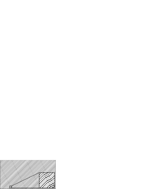
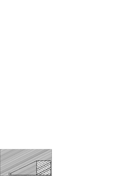
Figure 15: Time-space diagrams of the VDR-TCA model with $p_{0}=0.0$ and $p=1.0$. The shown lattices each contain 300 cells (corresponding to 2.25 km), the visible time horizon is always 580 seconds. The upper diagram and lower diagrams have densities $k=\frac{1}{3}+\frac{1}{K}$ and $k=0.4$ respectively, corresponding to observations in density region (II), labeled dilutely congested traffic (DCT).

In order to calculate the second transition point, we again observe the histogram of Fig. 12. A vehicle’s space gap now alternates between 1 and 2 cells in density region (II). And because its speed alternates between 0 and 1 cell/s respectively, the vehicles’ motions are controlled by cases (2) and (4a) from section IV.2. This means that stopped vehicles accelerate again in the next time step, after which they have to stop again, and so indefinitely repeating this cycle of stop-and-go behavior.

Consider now a pair of adjacent driving vehicles $i$ and $j$; it then follows from equation (1) that $h_{s_{i}}=1+1=2$ cells and $h_{s_{j}}=1+2=3$ cells. So each pair of vehicles ‘occupies’ 5 cells in the lattice, or 2.5 cells on average per vehicle. This leads to the second transition point being located at:

$$k_{(II)\rightarrow(III)}=\overline{h}_{s}^{-1}=\frac{1}{2.5}=0.4.$$ (15)

As the density is increased towards $k_{(II)\rightarrow(III)}$, the space mean speed decreases non-linearly. At the transition point itself, $\overline{v}_{s}=0.5$ cells/s and the system is now completely dominated by backward propagating dilute jams.

IV.5.3 Region (III) – densely advancing traffic [DAT]

Adding one more vehicle at the transition point between regions (II) and (III), leads to surprising behavior: a forward moving jam emerges, traveling at a speed of 0.5 cells/s (see Fig. 16). Another artefact is that the cycle of alternating space gaps of 1 and 2 cells, is broken with the introduction of a zero space gap at the location of this new ‘jam’. When the density reaches the third transition point, the system is completely filled with these forward moving ‘jams’ of dense traffic, leading to the description of ‘densely advancing traffic’ (DAT). Because the available space is more optimally used by the vehicles, an increase of the density thus has a (temporary) beneficial effect on the global flow measured in the system. This kind of behavior of forward moving density structures can also be observed in some models of anticipatory driving Lárraga et al. (2004).

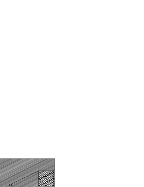
Figure 16: Time-space diagrams of the VDR-TCA model with $p_{0}=0.0$ and $p=1.0$. The shown lattices each contain 300 cells (corresponding to 2.25 km), the visible time horizon is always 580 seconds. The upper diagram and lower diagrams have densities $k=0.4+\frac{1}{K}$ and $k=\frac{2}{3}$ respectively, corresponding to observations in density region (III), labeled densely advancing traffic (DAT).

At the transition point itself, all vehicles exhibit the same behavior, comparable to the behavior at the second transition point. Traffic is more dense, as can be seen in the distribution of the space gaps in Fig. 12: all vehicles have alternatingly $g_{s}=0$ and $g_{s}=1$ cell (with corresponding speeds of 0 and 1 cell/s respectively). One pair of adjacent driving vehicles $i$ and $j$ thus ‘occupies’ $h_{s_{i}}+h_{s_{j}}=(1+0)+(1+1)=3$ cells, or 1.5 cells on average per vehicle. The third transition point thus corresponds to:

$$k_{(III)\rightarrow(IV)}=\overline{h}_{s}^{-1}=\frac{1}{1.5}=\frac{2}{3}.$$ (16)

IV.5.4 Region (IV) – heavily congested traffic [HCT]

Finally, as the system’s global density is pushed towards the jam density, each extra vehicle introduces at any point in time a backward propagating jam, consisting of a block of 5 consecutively stopped vehicles (see Fig. 17). The pattern of stable stop-and-go traffic gets destroyed, as vehicles remain stopped inside jams for longer time periods (cfr. density region (IV) in the distribution of the time gaps in Fig. 13), leading to the description of this traffic regime as ‘heavily congested traffic’ (HCT).

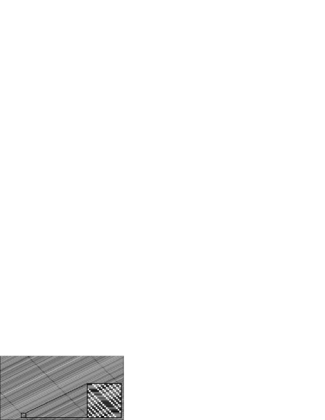
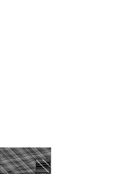
Figure 17: Time-space diagrams of the VDR-TCA model with $p_{0}=0.0$ and $p=1.0$. The shown lattices each contain 300 cells (corresponding to 2.25 km), the visible time horizon is always 580 seconds. The upper diagram and lower diagrams have densities $k=\frac{2}{3}+\frac{1}{K}$ and $k=0.85$ respectively, corresponding to observations in density region (IV), labeled heavily congested traffic (HCT).

IV.6 Varying the maximum speed

Up till now, the paper focused on VDR-TCA model’s behavior when $p_{0}=0.0$ and $p=1.0$, for $v_{\mbox{max}}=5$ cells/s. We can now ask the question: ”What would be the effect if we consider a lower maximum speed ?”

Considering the ($k$,$q$) fundamental diagrams in Fig. 18, we can see that a lower maximum speed has the significant effect of seemingly losing the first two transitions points $k_{(I)\rightarrow(II)}$ and $k_{(II)\rightarrow(III)}$. Put more correctly, when $v_{\mbox{max}}=1$ cell/s, the first transition point $k_{(I)\rightarrow(II)}$ gets drastically shifted towards a higher density of $\frac{2}{3}$. A side-effect is that the second and third transitions points vanish. This effect is also visible in the ($k$,$\overline{v}_{s}$) fundamental diagrams in Fig. 19. Note that we have set $p=0.9$ in order to make the differences between the fundamental diagrams more pronounced.

\psfrag{Global density k}{\footnotesize{Global density $k$}}\psfrag{Flow q [vehicles/hour]}{\footnotesize{Flow $q$ [vehicles/h]}}\psfrag{vMax = 1}{\footnotesize{$v_{\mbox{max}}=1$}}\psfrag{vMax = 2}{\footnotesize{$v_{\mbox{max}}=2$}}\psfrag{vMax = 5}{\footnotesize{$v_{\mbox{max}}=5$}}\includegraphics[width=244.69386pt]{Figures/FundamentalDiagrams/vdrtca/fundamental-diagrams-k-q-vdrtca-c1000-s500-tp1000-sp10000-vmax125-sp0.9-s2sp0.0.eps}

Figure 18: The ($k$,$q$) fundamental diagrams of the VDR-TCA with fixed slow-to-start and slowdown probabilities of $p_{0}=0.0$ and a $p=0.9$ respectively. The maximum speed was set at 1, 2, and 5 cells/s.

\psfrag{Global density k}{\footnotesize{Global density $k$}}\psfrag{Speed v [cells/s]}{\footnotesize{Space mean speed $\overline{v}_{s}$ [cells/s]}}\psfrag{vMax = 1}{\footnotesize{$v_{\mbox{max}}=1$}}\psfrag{vMax = 2}{\footnotesize{$v_{\mbox{max}}=2$}}\psfrag{vMax = 5}{\footnotesize{$v_{\mbox{max}}=5$}}\includegraphics[width=244.69386pt]{Figures/FundamentalDiagrams/vdrtca/fundamental-diagrams-k-v-vdrtca-c1000-s500-tp1000-sp10000-vmax125-sp0.9-s2sp0.0.eps}

Figure 19: The ($k$,$\overline{v}_{s}$) fundamental diagrams of the VDR-TCA with fixed slow-to-start and slowdown probabilities of $p_{0}=0.0$ and a $p=0.9$ respectively. The maximum speed was set at 1, 2, and 5 cells/s.

A decrease of the maximum speed thus has only a significant effect in the limiting case where $v_{\mbox{max}}=1$ cell/s, leading to a less rich dynamical behavior in the system. Any other maximum speed $v_{\mbox{max}}>1$ cell/s gives rise to different traffic regimes. Note that all the branches in the congested regions of the fundamental diagrams coincide once the first transition between regions (I) and (II) occurs at $k_{(I)\rightarrow(II)}=\frac{1}{3}$.

IV.7 Tracking the phase transitions

In order to track the transitions that occur between the different regimes (I)–(IV), we look for a suitable order parameter that expresses a qualitative behavior that changes between these regimes. In the following paragraphs, we describe the use of two such parameters: the first one is based on correlations between neighboring cells, whereas the second one is based on a comparison of the difference between the system’s global and local densities.

IV.7.1 Nearest neighbor correlations

One example of such a suitable measure, is the nearest neighbor order parameter $M_{1}$, which gives the time-space averaged density of those vehicles with speed $v=0$ cells/s which had to brake due to the next vehicle ahead Eisenblätter et al. (1998); Schadschneider (2002).

If we define the occupancy $\eta_{i}$ of cell $i$ as:

$$\left\{\begin{array}[]{lcl}\eta_{i}=1&\Leftrightarrow&\mbox{cell $i$ is occupied by a vehicle},\\ \eta_{i}=0&\Leftrightarrow&\mbox{cell $i$ is empty},\end{array}\right.$$ (17)

then we can define the order parameter $M_{1}$ as the following function that captures the density correlation between pairs of nearest neighbors (at a certain global density $k$):

$$M_{1}=\left<\frac{1}{K}\sum_{i=1}^{K}\eta_{i}\eta_{i+1}\right>_{T_{\mbox{sim}}},$$ (18)

with $\eta_{K+1}\equiv\eta_{1}$. Note that equation (18) is calculated as an average over the total simulation period $T_{\mbox{sim}}$. Figure 20 shows the results from an experiment for calculating $M_{1}$ when $K=300$ cells, $v_{\mbox{max}}=5$ cells/s and $T_{\mbox{sim}}=10^{5}$ s (with a transient period of $10^{3}$ s).

\psfrag{Global density k}{\footnotesize{Global density $k$}}\psfrag{Order parameter M1}{\footnotesize{Order parameter $M_{1}$}}\psfrag{p0 = 0.01 p = 0.50}{\footnotesize{$p_{0}=0.01$ $p=0.5$}}\psfrag{p0 = 0.00 p = 1.00}{\footnotesize{$p_{0}=0.0$ $p=1.0$}}\includegraphics[width=244.69386pt]{Figures/OrderParameters/vdrtca/nn-order-parameter-vdrtca-c300-s150-tp1000-sp100000-vmax5.eps}

Figure 20: The $M_{1}$ nearest neighbor order parameter for the two systems with $(p_{0},p)=(0.5,0.01)$ and $(p_{0},p)=(0.0,1.0)$ respectively. The system size was 300 cells and the total simulation period $T_{\mbox{sim}}=10^{5}$ s.

For the normal case where $p_{0}=0.5$ and $p=0.01$, we can see that $M_{1}$ is clearly able to detect the transition at the critical density: the order parameter shows a sudden significant increase. Although the VDR-TCA model exhibits metastability, it has only two distinct phases, namely free-flowing and jammed. These two phases are detected by the order parameter as it is constantly zero in the former, whereas it’s a linearly increasing function of the density in the latter. As stated, in the free-flowing regime, the nearest neighbor correlations are always zero because all the vehicles have large enough space gaps (i.e., at least the cell immediately in front of a vehicle is always empty).

If we consider the behavior of the order parameter $M_{1}$ in the second case, where $p_{0}=0.0$ and $p=1.0$, we see that it is not able to detect the first transition at $k_{(I)\rightarrow(II)}=\frac{1}{3}$. The reason for this can be determined by looking at the tempo-spatial evolutions in Figs. 14 and 15. Here we can see that, as described in sections IV.5.1 and IV.5.2, each vehicle always has at least one empty cell in front of it, leading to a nearest neighbor density correlation of zero.

The order parameter is however succesful in detecting the second transition at $k_{(II)\rightarrow(III)}=0.4$. The third transition at $k_{(III)\rightarrow(IV)}=\frac{2}{3}$ is detected, but in a non-intuitive manner: only the slope of the linear dependency between $M_{1}$ and $k$ changes when going from region (III) to region (IV).

We conclude this paragraph by stating that the $M_{1}$ order parameter is able to capture some transitions between different traffic regimes, but not all of them. Furthermore, it seems that the ability of the parameter to distinguish between two regimes is qualitively inferior: this can be witnessed by the weak behavioral change at the transition point $k_{(III)\rightarrow(IV)}$.

IV.7.2 A measure of inhomogeneity

A more suitable order parameter that can accurately track the transitions between the different regimes, is the order parameter $M_{2}$ defined by Jost and Nagel Jost and Nagel (2003). They partition the road into $L$ equal segments of integral length $K/L$. After calculating the local densities $k_{l_{i}}$ for all these segments $i$, they consider the variance of the local densities as their order parameter :

$$M_{2}=\left<\frac{1}{L}\sum_{i=1}^{L}(k_{l_{i}}-\mbox{E}[k_{l}])^{2}\right>_{T_{\mbox{sim}}}.$$ (19)

In equation (19), $\mbox{E}[k_{l}]$ denotes the expected value of the local density, which is equal to the global density $k$ because we consider a closed system. The local densities are calculated as:

$$k_{l_{i}}=\frac{1}{K/L}\sum_{j=i_{1}}^{j=i_{K/L}}\eta_{j},$$ (20)

with $i_{1}$ and $i_{K/L}$ denoting respectively the beginning and ending of segment $i$. The order parameter $M_{2}$ thus effectively tracks the differences in densities of individual segments, leading to a measure for the inhomogeneity in the system.

Note that $M_{2}$ is calculated as an average over $T_{\mbox{sim}}$ time steps, just as was done for the previous order parameter $M_{1}$. This means that we calculated the summation in equation (19) at each time step, and averaged all these results over a simulation period of $T_{\mbox{sim}}$. Care should be taken not to prematurely average the local densities over more than one time step, as this would significantly deteriorate the tracking quality of the order parameter: the longer the aggregation period for calculating the local densities, the more each segment ‘sees’ the densities recorded in the other segments as congestion waves are traveling around the closed system.

In Fig. 21 we can see the results for different slowdown probabilities $p$ (the slow-to-start probability $p_{0}$ was fixed at 0.0). The system size $K$ was set to 300 cells, $v_{\mbox{max}}=5$ cells/s and $T_{\mbox{sim}}=10^{5}$ s (with a transient period of $10^{3}$ s).

\psfrag{Global density k}{\footnotesize{Global density $k$}}\psfrag{Inhomogeneity measure M2}{\footnotesize{Inhomogeneity measure $M_{2}$}}\psfrag{p = 0.10}{\footnotesize{$p=0.10$}}\psfrag{p = 0.25}{\footnotesize{$p=0.25$}}\psfrag{p = 0.50}{\footnotesize{$p=0.50$}}\psfrag{p = 0.75}{\footnotesize{$p=0.75$}}\psfrag{p = 0.90}{\footnotesize{$p=0.90$}}\psfrag{p = 1.00}{\footnotesize{$p=1.00$}}\includegraphics[width=244.69386pt]{Figures/OrderParameters/vdrtca/inhomogeneity-measure-vdrtca-c300-s150-tp1000-sp100000-vmax5.eps}

Figure 21: The $M_{2}$ order parameter which measures the variance of the local densities. In each diagram, the slow-to-start probability $p_{0}$ was fixed at 0.0, whereas the slowdown probability $p$ was varied between 0.1 and 1.0 (the system size was 300 cells and the total simulation period $T_{\mbox{sim}}=10^{5}$ s). The thick line denotes the limiting case where $p_{0}=0.0$ and $p=1.0$.

From the graph of $M_{2}$ with $p_{0}=0.0$ and $p=1.0$, it is interesting to notice that this order parameter performs exquisitely well at tracking the transitions between the different traffic regimes. Each time a transition point is encountered, $M_{2}$ drops to zero. This specific behavior of the order parameter can be understood by looking at the tempo-spatial conditions that hold at these transitional densities: each time, the system settles in a complete homogeneous equilibrium (as can be seen from the lower time-space diagrams in Figs. 14, 15 and 16). The distribution of the vehicles’ space gaps (Fig. 12) also has a variance of zero at the first transition point, but not at the others. We thus conclude that this inhomogeneity measure is able to accurately track the four previously discussed phase transitions.

V Comparison with existing literature

A final word should be said about the behavior of the four phases discussed in this paper. Although the study is based on a well-known traffic flow model (i.e., the VDR-TCA model), it seems that this behavior is drastically different from that observed in real-life traffic. The research elucidated in this paper, is therefore relevant as it can be compared to phase transitions in other types of granular media, described by cellular automata.

Relating our findings to similar considerations in literature, we note the following aspects: Grabolus Grabolus (2001) gives a thorough discussion of several variants of the STCA, including so-called ‘fast-to-start’ TCA models that give rise to forward propagating density waves; the study refers to the two-fluid theory Williams (1997) as a possible explanation of this phenomenon. Gray and Griffeath Gray and Griffeath (2001) discuss the origin of non-concavity in the ($k$,$q$) fundamental diagram, where they propose an explanation in which the rear end of a jam is unstable, whereas its front is stable and growing. Leveque Leveque (2001) incorporates a non-concave fundamental diagram itself in a macroscopic model, thereby resembling night driving. Nishinari et al Nishinari et al. (2003) consider the tempo-spatial organization of ants using an ant trail model based on pheromones. In their model, the average speed of the ants varies non-monotonically with their density, leading to an inflection point in the ($k$,$q$) fundamental diagram. Zhang Zhang (2003) questions the property of anisotropy in multi-lane traffic, leading to strikingly similar non-concave ($k$,$q$) fundamental diagrams.

Finally, Awazu Awazu (1999) investigated the flow of various complex particles using a simple meta-model based on Wolfram’s CA-rule 184, but extended with rules that govern the change in speed of individual particles. As a result, he classified three types of fundamental diagrams, namely two phases (2P), three phases (3P), and four phases (4P) type systems. Of these types, the 4P-type complex granular particle systems closely resemble the regimes discovered in this paper. Awazu discusses the types of regimes and the transitions between them, using the terminology of ‘dilute slugs’ for the slow moving jams in the DCT-phase (see section IV.5.2), which he calls the ‘dilute jam-flow state’. Analogously, there are ‘advancing slugs’ in the ‘advancing jam-flow state’ (related to our DAT-phase in section IV.5.3) and the fourth phase is called the ‘hard jam-flow state’ (related to our HCT-phase in section IV.5.4).

As stated before, the behavior here is different from that of real-life traffic flows. Awazu expects that these transitions appear if there are more complex interactions between the particles. In the 4P-type systems, attractive forces between close neighbouring particles and an effective resistance on moving neighbouring particles, lead to the realization of the previously discussed flow phases.

VI Summary

In this paper, we first showed the behavioral characteristics resulting from the velocity dependent randomization traffic cellular automaton (VDR-TCA) model, operating under normal conditions (i.e., $p_{0}\gg p$). Then we investigated the more complex system dynamics that arise from this traffic flow model in the exceptional cases when $p_{0}\ll p$. This behavior was quantitavely compared against the VDR-TCA’s normal operation, using classical fundamental diagrams and histograms that show the distribution of the speeds, space, and time gaps.

Our main investigations were primarily directed at the limiting case where $p_{0}=0.0$ and $p=1.0$. We discovered the emergence of four different traffic regimes. These regimes were individually studied using diagrams that show the evolution of their tempo-spatial behavioral characteristics. This resulted in the following classification: free-flowing traffic (FFT), dilutely congested traffic (DCT), densely advancing traffic (DAT), and heavily congested traffic (HCT). Our main conclusions here are:

• all four phases share the common property that moving vehicles can never increase their speed once the system has settled into an equilibrium,

• the DAT regime experiences forward propagating density waves, corresponding to a non-concave region in the system’s flow-density relation.

In order to track the phase transitions between these traffic regimes, we looked at two order parameters: the first one $M_{1}$ was based on correlations between neighboring cells, whereas the second one $M_{2}$ was based on a comparison of the difference between the system’s global and local densities. We concluded that, as opposed to $M_{1}$, this latter order parameter $M_{2}$ performs exemplary at tracking the transitions between the different traffic regimes.

Comparing our results with those in existing literature, we conclude that the work of Awazu Awazu (1999), dealing with a cellular automaton model of various complex particles, gives the closest resemblance to our four phases.

References

- Maerivoet and Moor (2003) S. Maerivoet and B. D. Moor, in Proceedings of the 10th World Congress and Exhibition on Intelligent Transport Systems and Services (CD-ROM) (ERTICO, ITS Europe, Madrid, Spain, 2003).
- Nagel and Schreckenberg (1992) K. Nagel and M. Schreckenberg, Journal de Physique I France 2, 2221 (1992).
- Nagel (1994) K. Nagel, International Journal of Modern Physics C 5, 567 (1994).
- Takayasu and Takayasu (1993) M. Takayasu and H. Takayasu, Fractals 1 pp. 860–866 (1993).
- Barlović et al. (1998) R. Barlović, L. Santen, A. Schadschneider, and M. Schreckenberg, European Physics Journal B5 (1998).
- Awazu (1999) A. Awazu, Physics Letters A 261, 309 (1999).
- Grabolus (2001) S. Grabolus, Master’s thesis, Institut für Theoretische Physik, Universität zu Köln (2001).
- Gray and Griffeath (2001) L. Gray and D. Griffeath, Journal of Statistical Physics 105, 413 (2001).
- Leveque (2001) R. J. Leveque, in Minisymposium on traffic flow, (SIAM Annual Meeting, 2001).
- Nishinari et al. (2003) K. Nishinari, D. Chowdhury, and A. Schadschneider, Physical Review E 67, 036120 (2003).
- Zhang (2003) H. Zhang, Transportation Research B 37B, 561 (2003).
- Nagel (1995) K. Nagel, Ph.D. thesis, Universität zu Köln (1995).
- Chowdhury et al. (1998) D. Chowdhury, A. Pasupathy, and S. Sinha, European Physics Journal B - Condensed Matter 5, 781 (1998).
- Schadschneider (2000) A. Schadschneider, Physica A p. 101 (2000).
- Helbing (2001) D. Helbing, Review of Modern Physics 73, 1067 (2001).
-
Maerivoet (2004)
S. Maerivoet,
Traffic Cellular Automata,
Java software tested with JDK 1.3.1
(2004),
(URL : http://smtca.dyns.cx). - Chowdhury et al. (2000) D. Chowdhury, L. Santen, and A. Schadschneider, Physics Reports 329, 199 (2000).
- Barlović et al. (1999) R. Barlović, J. Esser, K. Froese, W. Knospe, L. Neubat, M. Schreckenberg, and J. Wahle, Traffic and Mobility : Simulation-Economics-Environment pp. 117–134 (1999), Institut für Kraftfahrwesen, RWTH Aachen, Duisburg.
- Wolfram (2002) S. Wolfram, A New Kind of Science (Wolfram Media, Inc., 2002), ISBN 1-579-955008-8.
- Schadschneider (2002) A. Schadschneider, Physica A 313, 153 (2002).
- Maerivoet et al. (2003) S. Maerivoet, S. Logghe, B. D. Moor, and B. Immers, in Proceedings of the Workshop on Traffic and Granular Flow ’03 (Delft University of Technology, Delft, The Netherlands, 2003).
- Lárraga et al. (2004) M. Lárraga, J. del Río, and A. Schadschneider, Journal of Physics A: Mathematical and General pp. 3769–3781 (2004).
- Schreckenberg et al. (2001) M. Schreckenberg, R.Barlović, W. Knospe, and H. Klüpfel, in Computational Statistical Physics, edited by K. H. Hoffmann and M. Schreiber (Springer, Berlin, 2001), pp. 113–126.
- Eisenblätter et al. (1998) B. Eisenblätter, L. Santen, A. Schadschneider, and M. Schreckenberg, Physical Review E 57, 1309 (1998).
- Jost and Nagel (2003) D. Jost and K. Nagel, in Transportation Research Board Annual Meeting (Washington, D.C., 2003), Paper 03-4266.
- Williams (1997) J. C. Williams, in Traffic Flow Theory: A State-of-the-Art Report, edited by N. Gartner, H. Mahmassani, C. J. Messer, H. Lieu, R. Cunard, and A. K. Rathi, Federal Highway Administration (Transportation Reseach Board, 1997), pp. 6.17–6.29.
- Lighthill and Whitham (1955) M. Lighthill and G. Whitham, in Proceedings of the Royal Society (1955), vol. A229, pp. 317–345.