Diffusion of passive scalar in a finite-scale random flow

Abstract

We consider a solvable model of the decay of scalar variance in a single-scale random velocity field. We show that if there is a separation between the flow scale $k_{\text{flow}}^{-1}$ and the box size $k_{\text{box}}^{-1}$, the decay rate $\lambda\propto(k_{\text{box}}/k_{\text{flow}})^{2}$ is determined by the turbulent diffusion of the box-scale mode. Exponential decay at the rate $\lambda$ is preceded by a transient powerlike decay (the total scalar variance $\sim t^{-5/2}$ if the Corrsin invariant is zero, $t^{-3/2}$ otherwise) that lasts a time $t\sim 1/\lambda$. Spectra are sharply peaked at $k=k_{\text{box}}$. The box-scale peak acts as a slowly decaying source to a secondary peak at the flow scale. The variance spectrum at scales intermediate between the two peaks ($k_{\text{box}}\ll k\ll k_{\text{flow}}$) is $\sim k+ak^{2}+\dots$ ($a>0$). The mixing of the flow-scale modes by the random flow produces, for the case of large Péclet number, a $k^{-1+\delta}$ spectrum at $k\gg k_{\text{flow}}$, where $\delta\propto\lambda$ is a small correction. Our solution thus elucidates the spectral make up of the “strange mode,” combining small-scale structure and a decay law set by the largest scales.

I Introduction

The problem of the decay of passive-scalar variance has recently been reexamined in the literature following the realization that the decay rates, spectra, and higher-order statistics based on small-scale Lagrangian-stretching theories Antonsen et al. (1996); Son (1999); Balkovsky and Fouxon (1999); Falkovich et al. (2001) are not consistent with either numerical Pierrehumbert (1994, 2000); Fereday et al. (2002); Sukhatme and Pierrehumbert (2002) or experimental Rothstein et al. (1999); Voth et al. (2003) results in the long-time limit. Instead, the scalar decay is dominated by an eigenmodelike solution dubbed “the strange mode” Pierrehumbert (1994) because it combines intricate small-scale structure with globally determined decay rate and self-similar statistics (self-similarity is also seen in numerical simulations of the related problem of kinematic dynamo Schekochihin et al. (2004)). There has been a growing understanding Voth et al. (2003); Thiffeault and Childress (2003); Chertkov and Lebedev (2003); Fereday and Haynes (2004); Sukhatme (2004) that the overall decay rate is set by the slowest-decaying system-scale modes. This brings to mind homogenization theory Majda and Kramer (1999), which considers the turbulent diffusion of passive scalar at scales much larger than the flow scale and where it is the largest-scale mode that decays most slowly. In this paper, we use a simple solvable example to demonstrate that the strange-mode decay rate is the rate of turbulent diffusion of the box-scale mode and show how the spectra of scalar variance accommodate both this box-scale diffusion and small-scale structure.

Qualitatively, the key idea quantified by our theory is as follows. A scalar field whose variance is at the scale smaller than or equal to the scale of the ambient random flow is mixed at a rate determined by the Lyapunov exponent of the flow — this is the Lagrangian-stretching approach. However, if the size of the box is larger than the scale of the flow, the scalar field can have variance at the scale of the box. The rate of transfer of this large-scale variance to the flow scale (turbulent diffusion) can be much smaller than the Lagrangian mixing rate, in which case this slow transfer sets the global decay rate.

Our model emphasizes scale separation between the box and the flow. Our results are complementary to Haynes and Vanneste (2005), where the decay of a scalar field is studied with more generality (in two dimensions).

We consider the advection-diffusion equation

$$\partial_{t}\theta+{\bf u}\cdot\nabla\theta=\eta\Delta\theta,$$ (1)

with a random Gaussian white-in-time velocity field $\langle u^{i}(t,{\bf x})u^{j}(t^{\prime},{\bf x}^{\prime})\rangle=\delta(t-t^{\prime})\kappa^{ij}({\bf x}-{\bf x}^{\prime})$ known as the Kraichnan model Kraichnan (1968). The mean scalar concentration has been subtracted — i.e., $\langle\theta\rangle=0$. For the Kraichnan velocity, the angle-integrated scalar-variance spectrum in $d$ dimensions $T(k)=\int d\Omega_{\bf k}\,k^{d-1}\langle|\theta({\bf k})|^{2}\rangle$ satisfies an integro-differential equation valid at all $k$ :

$$\partial_{t}T(t,k) + (2\eta+\kappa_{0})k^{2}T(t,k)$$ (2)

$$= k_{i}k_{j}\int d^{d}k^{\prime}\kappa^{ij}({\bf k}-{\bf k}^{\prime})\,T(t,k^{\prime}),$$

where ${\hat{\kappa}}^{ij}({\bf k})={\hat{\kappa}}(k)\bigl{(}\delta^{ij}-k_{i}k_{j}/k^{2}\bigr{)}$ is the Fourier transform of $\kappa^{ij}({\bf x}-{\bf x}^{\prime})$ and $\kappa_{0}=(1/d)\kappa^{ii}(0)$ is the turbulent diffusivity ($d$ is the dimension of space).

In Sec. II, we review the theory of scalar decay at small scales, which leads to the standard Lagrangian-stretching results. In Sec. III, the theory for a finite-scale flow is developed — this is the main part of the paper. Concluding remarks are in Sec. IV.

II Small-scale theory

If the Péclet number $\text{Pe}=uk_{\text{flow}}^{-1}/\eta$ is large, $\theta$ varies at scales as small as $\text{Pe}^{-1/2}$ times the scale of the flow. This small-scale structure can be considered in the approximation of spatially linear velocity field Batchelor (1959); Kraichnan (1974), — viz.,

$$\kappa^{ij}({\bf y})\simeq\kappa_{0}\delta^{ij}-{1\over 2}\,\kappa_{2}\left(y^{2}\delta^{ij}-{1\over 2}\,y^{i}y^{j}\right).$$ (3)

For the Kraichnan velocity, the Lagrangian-stretching theories Antonsen et al. (1996); Son (1999); Balkovsky and Fouxon (1999); Falkovich et al. (2001) amount to the approximation (3). The scalar-variance spectrum satisfies a Fokker-Planck-type equation Kraichnan (1968, 1974)

$$\partial_{t}T=D\,{\partial\over\partial k}\left[k^{2}{\partial T\over\partial k}-(d-1)kT\right]-2\eta k^{2}T,$$ (4)

where $D=[(d-1)/2(d+1)]\kappa_{2}$. This equation is valid for $k\gg k_{\text{flow}}$. In this limit, it either can be obtained from Eq. (2) by expanding the mode-coupling term on the right-hand side or derived directly by assuming linear velocity field Kraichnan (1974).

The solution of Eq. (4) that decays at $k\to\infty$ is

$$T(t,k)={C_{\lambda}}\,e^{-\lambda\gamma_{0}t}k^{-1+d/2}K_{(d/2)\sqrt{1-\lambda}}\,(k/k_{\eta}),$$ (5)

where ${C_{\lambda}}$ is a constant, $K_{\nu}(z)$ is the modified Bessel function of the second kind, $\gamma_{0}=(d^{2}/4)D$, $k_{\eta}=(D/2\eta)^{1/2}$, and $\lambda$ is the nondimensionalized decay rate, which must be calculated by applying the correct boundary condition at small $k$. If we assumed that the decay rate is fully determined by the small scales, a reasonable procedure would be to choose some infrared cutoff $k_{*}$ and require the flux of scalar variance through $k_{*}$ [the square brackets in Eq. (4)] to vanish (cf. Schekochihin et al. (2002a)). This can be satisfied only for $\lambda>1$. For $k_{*}\ll k_{\eta}$, the zero-flux condition becomes $\sin\bigl{[}(d/2)\sqrt{\lambda-1}\,\ln(k_{*}/2k_{\eta})\bigr{]}=0$. Placing the cutoff $k_{*}$ at the largest zero, ensures that $T(k)$ is everywhere positive. We get (cf. Haynes and Vanneste (2005))

$$\lambda=1+{(2\pi/d)^{2}\over\bigl{[}\ln(k_{*}/2k_{\eta})\bigr{]}^{2}}=1+O\bigl{(}1/\log^{2}\text{Pe}\bigr{)}.$$ (6)

This implies a $k^{(d-2)/2}$ spectrum at $k\gg k_{\eta}$. If the scalar variance is initially at $k\gg k_{\text{flow}}$, these results (or their analogs for other model flows) hold during the initial stage of the scalar decay. However, in the long-time limit for cases in which the system (box) size is (several times) larger than the flow scale, both numerical simulations Fereday and Haynes (2004) and experimental results Voth et al. (2003) obtain much smaller decay rates and spectra with negative exponents. The conclusion is that the zero-flux boundary condition is incorrect and the decay rate $\lambda<1$ must be determined by matching the solution (5) to the solution at nonlarge $k$ where Eq. (4) is invalid and Eq. (2) must be used instead. The spectrum at $k_{\text{flow}}\ll k\ll k_{\eta}$ is then $\sim k^{s(\lambda)}$, where [from Eq. (5)]

$$s(\lambda)=-1+(d/2)\bigl{(}1-\sqrt{1-\lambda}\bigr{)}.$$ (7)

Note that for $\lambda\ll 1$, $s(\lambda)\simeq-1+(d/4)\lambda$, which coincides with the formula proposed in Fereday and Haynes (2004).

For the initial spectrum concentrated at $k\sim k_{\eta}$, the period of validity of Eq. (6) is the time it takes the spectrum to spread to $k\sim k_{\text{flow}}$. The spreading can be shown to be exponentially fast with a rate $\sim\gamma_{0}$. Since $k_{\eta}\sim\text{Pe}^{1/2}k_{\text{flow}}$, the Lagrangian-stretching results are valid for $t\ll\gamma_{0}^{-1}\log\text{Pe}$.

III Theory for a finite-scale flow

The challenge now is to find $\lambda$ by solving Eq. (2). Let us specialize to three dimensions (theory in 2D is analogous) and choose a simple form for the velocity correlator: ${\hat{\kappa}}(k)=N\,\delta(k-k_{\text{flow}})$, where $N=15\kappa_{2}/16\pi k_{\text{flow}}^{4}$ [note that $\kappa_{2}=(2/5)k_{\text{flow}}^{2}\kappa_{0}$]. This describes a Kraichnan ensemble of randomly oriented “eddies” of size $k_{\text{flow}}$. We set $k_{\text{flow}}=1$ and carry out angle integrations in Eq. (2) to get

$$\partial_{t}T(t,k) + (2\eta+\kappa_{0})k^{2}T(t,k)$$ (8)

$$= {15\over 32}\,\kappa_{2}\,k\int_{|1-k|}^{1+k}{dk^{\prime}\over k^{\prime}}\,K(k,k^{\prime})T(t,k^{\prime}),$$

where $K(k,k^{\prime})=-k^{\prime 4}+2(1+k^{2})k^{\prime 2}-(1-k^{2})^{2}$. It is not hard to ascertain that Eq. (8) reduces to Eq. (4) when $k\gg 1$. Let us now consider the opposite limit $k\ll 1$ — i.e., the evolution of scale variance at scales much larger than the scale of the flow. In this limit, the integral in Eq. (8) is dominated by the modes in the neighborhood of the flow scale $k=1$. Neglecting $\eta$, we get

$$\partial_{t}T+k^{2}T={3\over 4}\,k\int_{-k}^{k}dq\,(k^{2}-q^{2})T(t,1+q)\equiv S(t,k),$$ (9)

where time is rescaled $t\kappa_{0}k_{\text{flow}}^{2}\to t$. The solution is

$$T(t,k)=\left[T(0,k)+\int_{0}^{t}dt^{\prime}S(t^{\prime},k)e^{k^{2}t^{\prime}}\right]e^{-k^{2}t}.$$ (10)

In order to complete the solution, we must determine $T(t,1+q)$. For $q\ll 1$, it satisfies

$$\partial_{t}T+T={3\over 4}\,\int_{|q|}^{2+q}{dk^{\prime}\over k^{\prime}}\left(k^{\prime 2}-{k^{\prime 4}\over 4}-q^{2}\right)T(t,k^{\prime}).$$ (11)

As we shall see, the solution (10) is sharply peaked at $k=k_{\text{peak}}\sim 1/\sqrt{t}$. In an infinite system, this peak would move indefinitely towards ever smaller $k$. In a finite system, $k_{\text{peak}}$ eventually becomes comparable to the inverse system size. Strictly speaking, this means that one must solve the problem with a discrete set of modes and application-specific boundary conditions (cf. Chertkov and Lebedev (2003); Lebedev and Turitsyn (2004); Haynes and Vanneste (2005)). Instead, we model the finite box by introducing an infrared cutoff $k_{\text{box}}$ into our continuous theory. All lower integration limits in $k$ space are subject to this cutoff. This is not a rigorous operation, but it is a reasonable modeling choice as long as $k_{\text{box}}\ll 1$. The time at which $k_{\text{peak}}\sim k_{\text{box}}$ is $t\sim 1/k_{\text{box}}^{2}$. Therefore, there will be two asymptotic regimes of scalar decay: the transient stage $t\ll 1/k_{\text{box}}^{2}$, when unmodified continuous theory can be used, and the long-time limit $t\gg 1/k_{\text{box}}^{2}$, when the box cutoff is important. Note that even for the transient stage, we assume $t\gg 1$; i.e., we consider times much longer than the “turnover time” of the flow. For spectra initially at small scales, we harden this condition to $t\gg\log\text{Pe}$, so that the Lagrangian-stretching theory ceases to be valid.

Consider Eq. (10). Since $k\ll 1$, we can Taylor-expand the initial spectrum: $T(0,k)=C_{2}k^{2}+C_{4}k^{4}+\dots$. Here $C_{2}$ is the Corrsin invariant, $C_{2}\propto\int d^{3}x\,\langle\theta({\bf x})\theta(0)\rangle$ Corrsin (1951a). Some aspects of the scalar decay differ for cases with $C_{2}>0$ and $C_{2}=0$. We shall first develop our theory for $C_{2}>0$. The case of $C_{2}=0$ will be treated in Sec. III.4.

III.1 Case of $C_{2}>0$

Consider first the transient stage $1\ll t\ll 1/k_{\text{box}}^{2}$. Let us assume that the dominant term in the solution (10) is

$$T(t,k)=C_{2}k^{2}e^{-k^{2}t},$$ (12)

which peaks at $k_{\text{peak}}=1/\sqrt{t}$. We shall justify this assumption a posteriori. Let us now determine the flow-scale solution [Eq. (11)]. Assuming that the main contribution to the integral in Eq. (11) is from $k^{\prime}\ll 1$ (also to be verified later) and substituting Eq. (12) for $T(t,k^{\prime})$, we get, to leading order in in $1/t$ (and neglecting $\partial_{t}T$),

$$T(t,1+q)={3\over 8}\,{C_{2}\over t^{2}}\,e^{-q^{2}t}\equiv T_{1}(t)e^{-q^{2}t},$$ (13)

where $T_{1}(t)=T(t,1)$. This describes the neighborhood of the flow scale, where the coupling to the small-$k$ modes produces a secondary peak with the width $\sim 1/\sqrt{t}$. We shall see below that Eq. (13) is, in fact, valid beyond the width of the peak and up to $|q|\sim(\ln t/t)^{1/2}$. We now substitute Eq. (13) back into Eq. (10) to see that Eq. (12) is, indeed, the dominant solution.

For $k\ll 1/\sqrt{t}$, we get $S(t,k)\simeq k^{4}T_{1}(t)$. Equation (10) becomes, to two leading orders in $k$,

$$T(t,k)\simeq\left[C_{2}k^{2}+\left(C_{4}+\int_{0}^{t}dt^{\prime}T_{1}(t^{\prime})\right)k^{4}\right]e^{-k^{2}t}.$$ (14)

Since $T_{1}(t)$ decays faster than $1/t$ [Eq. (13)], its time integral in Eq. (14) tends to a constant when $t\gg 1$ and is dominated by the initial stage of the evolution of $T_{1}(t^{\prime})$ [there is no divergence at $t^{\prime}=0$ because the solution (13) is only valid for $t^{\prime}\gg 1$]. This time integral represents a finite amount of scalar variance that is initially transferred from the flow scale to the large scales (small $k$). That the effect of nonlinear coupling only appears in the $k^{4}$ term is a reflection of the conservation of the Corrsin invariant: the coefficient in front of $k^{2}$ cannot be changed. We see that, as long as $C_{2}\gg\text{const}\times k_{\text{box}}^{2}$, the first term in Eq. (14) dominates. Note that for $k\sim 1/\sqrt{t}$, it is still true that the time integral in Eq. (10) is $\sim k^{4}$, so the above estimates remain valid.

Now consider $1/\sqrt{t}\ll k\ll 1$. In this limit, $S(t,k)\simeq(3/4)\sqrt{\pi}\,T_{1}(t)t^{-1/2}k^{3}$. Substituting into Eq. (10), we get

$$T(t,k)\simeq C_{2}k^{2}e^{-k^{2}t}+{3\over 4}\,\sqrt{\pi}\,T_{1}(t)t^{-1/2}k.$$ (15)

The second term becomes comparable to the first at $k\sim(\ln t/t)^{1/2}$. At larger $k$ (but still $k\ll 1$), it replaces the solution (12) as the dominant asymptotic. The solution (15) is uniformly valid across the transition region. Together with Eq. (11), this implies that the solution (13) is valid for $|q|\lesssim(\ln t/t)^{1/2}$.

In the long-time limit $t\gg 1/k_{\text{box}}^{2}$, Eq. (10) is still valid. Again, we assume that the dominant solution is Eq. (12). Its peak is at $k_{\text{peak}}=k_{\text{box}}$. In Eq. (11), the lower integration limit is adjusted to $\max\{|q|,\,k_{\text{box}}\}$, as explained above. The flow-scale peak is now confined to $|q|<k_{\text{box}}$. At these $q$, Eq. (13) is replaced by

$$T(t,1+q)={3\over 8}\,{C_{2}\over t}\,(k_{\text{box}}^{2}-q^{2})\,e^{-k_{\text{box}}^{2}t}.$$ (16)

This solution gives the dominant contribution to $S(t,x)$ [Eq. (9)], so we have (integrating from $-k_{\text{box}}$ to $k_{\text{box}}$) $S(t,k)=(3/8)C_{2}t^{-1}k(k^{2}-k_{\text{box}}^{2}/5)k_{\text{box}}^{3}\exp(-k_{\text{box}}^{2}t)$, which we substitute into Eq. (10). The box mode obeys

$$T(t,k_{\text{box}})\simeq\left(C_{2}k_{\text{box}}^{2}+{3\over 10}\,C_{2}k_{\text{box}}^{6}\ln t\right)e^{-k_{\text{box}}^{2}t}.$$ (17)

The time integral now has a logarithmic divergence, representing a small amount of transfer of scalar variance from the flow-scale mode to the box mode. This contribution is not significant because the second term in Eq. (17) only exceeds the first at $t=\exp(10/3k_{\text{box}}^{4})$, which is unphysically large even for moderately small values of $k_{\text{box}}$. The width of the box-scale peak, for which the decay law (17) is valid, is estimated by $k^{2}-k_{\text{box}}^{2}\lesssim 1/t$ — i.e., $k-k_{\text{box}}\lesssim 1/2k_{\text{box}}t$.

Outside the peak $(k^{2}-k_{\text{box}}^{2})t\gg 1$, we have

$$T(t,k) \simeq C_{2}k^{2}e^{-k^{2}t}$$ (18)

$$+\,\,{3\over 8}\,{C_{2}\over t}\,k\,{k^{2}-k_{\text{box}}^{2}/5\over k^{2}-k_{\text{box}}^{2}}\,k_{\text{box}}^{3}e^{-k_{\text{box}}^{2}t}.$$

The first and second terms are of the same order when $k^{2}-k_{\text{box}}^{2}\sim\ln t/t$ — i.e., $k-k_{\text{box}}\sim\ln t/k_{\text{box}}t$. In the intermediate scale range $k_{\text{box}}\ll k\ll 1$, we have

$$T(t,k)\simeq{3\over 8}\,{C_{2}\over t}\,kk_{\text{box}}^{3}e^{-k_{\text{box}}^{2}t}=T_{1}(t)k_{\text{box}}k.$$ (19)

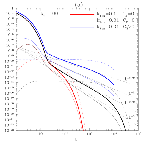
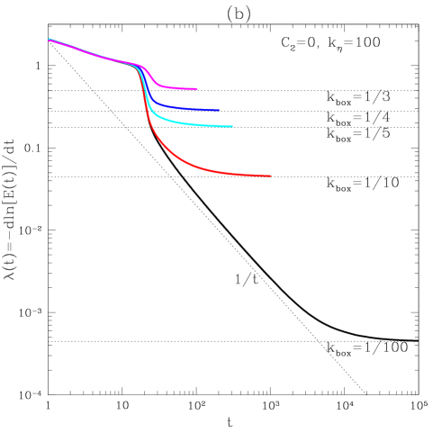
Figure 1: (a) Scalar-variance decay: bold lines depict the total variance $E(t)$, thin lines the flow-scale mode $T(t,1)$, and dashed lines the box mode $T(t,k_{\text{box}})$. Dotted lines are theoretical slopes. Time is in units of $\gamma_{0}^{-1}$. The $C_{2}=0$ runs are the same as in Fig. 2. (b) Effective decay rate $\lambda(t)=-d\ln E(t)/dt$. in units of the Lagrangian-stretching decay rate $\gamma_{0}$ for various values of $k_{\text{box}}$. Dotted lines correspond to $\lambda=(40/9)k_{\text{box}}^{2}$. The initial spectrum was the same as for Fig. 2.

Let us summarize what we have learned so far. We have been concerned with two narrow bands of modes: the flow-scale modes $T(t,1+q)$, $q\ll 1$, and the large-scale peak $T(t,k_{\text{peak}})$ at $k_{\text{peak}}=1/\sqrt{t}$, which became the box mode $T(t,k_{\text{box}})$ in the long-time limit $t\gg 1/k_{\text{box}}^{2}$. The width of the peak was $\sim 1/\sqrt{t}$ when $t\ll 1/k_{\text{box}}^{2}$ and $\sim 1/k_{\text{box}}t$ when $t\gg 1/k_{\text{box}}^{2}$. The flow-scale modes could be assumed to be coupled solely to the peak because of the peak’s sharp dominance of all other modes: indeed, $T(t,k_{\text{peak}})\sim tT_{1}(t)\gg T_{1}(t)$. The width of the secondary peak at the flow scale was determined by $k_{\text{peak}}$. This width can be parametrized by $\Lambda(t)=(k_{\text{box}}^{2}+1/t)^{1/2}$.

The large-scale peak and the flow-scale band are singularities of the scalar-variance spectrum. Note that in the long-time limit $t\gg 1/k_{\text{box}}^{2}$, the width of the flow-scale peak is $\Lambda=k_{\text{box}}$, while the width of the box mode is $1/k_{\text{box}}t\ll k_{\text{box}}$. In a finite system, the spacing of the modes cannot be smaller than $k_{\text{box}}$, so it is, of course, unphysical to talk about variation of the spectrum at distances less than $k_{\text{box}}$. In our continuous theory, the collapse of the singularities to profiles narrower than $k_{\text{box}}$ means that they should be interpreted as single modes. Formally, they can be represented as $\delta$ functions: thus, for the flow-scale band $1-\Lambda(t)<k<1+\Lambda(t)$, we write $T(t,k)=N_{1}T_{1}(t)\Lambda(t)\delta(k-1)$, where $N_{1}$ is a constant arising from integrating over the specific shape of the singularity: $N_{1}=\sqrt{\pi}$ in the transient stage and $N_{1}=4/3$ in the long-time limit.

III.2 Nonsingular spectrum

Let us now consider the nonsingular part of the spectrum. For all $k>\Lambda(t)$, we write

$$T(t,k)=N_{1}\Lambda(t)T_{1}(t)\bigl{[}\delta(k-1)+f(k)\bigr{]}.$$ (20)

Substituting this decomposition into Eq. (8) and neglecting $d\ln[\Lambda(t)T_{1}(t)]/dt$, we find the equation for $f(k)$:

$$\left(1+{1\over 10\,k_{\eta}^{2}}\right)f(k) = {3\over 4}\,k\left(1-{k^{2}\over 4}\right)H(2-k)$$ (21)

$$+ {3\over 16}\,{1\over k}\int_{|1-k|}^{1+k}{dk^{\prime}\over k^{\prime}}\,K(k,k^{\prime})f(k^{\prime}),\quad\quad$$

where $H(2-k)$ is the Heaviside step function [the term it multiplies comes from integrating $\delta(k-1)$ and vanishes for $k>2$]. For $k\ll 1$, we expand $f(k^{\prime})$ under the integral around $k^{\prime}=1$ and find that the lowest-order term is $f(1)k^{2}$. Clearly, $f(1)>0$. Thus, the spectrum at scales intermediate between the box scale and the flow scale is

$$T(t,k)=N_{1}\Lambda(t)T_{1}(t)\bigl{[}(3/4)k+f(1)k^{2}+\dots\bigr{]}.$$ (22)

Coefficients in higher-order terms will involve derivatives of $f$ at $k=1$. The first term in the expansion (22) comes from coupling to the flow-scale mode and is consistent with the asymptotics (15) and (19), so the nonsingular solution connects smoothly to the large-scale peak. The interaction of the nonsingular modes between themselves enters in the second order.

To complete the solution, we would have to find $f(k)$ at $k\geq 1$. For $k\leq 2$, this means solving the full integral equation, but we do not really need to do this. Note that the modes with $k>2$ are not directly coupled to the flow-scale mode. In a rough way, it can be said that the Fokker-Planck regime starts at $k=2$ and the solution of Eq. (4) must be matched to $T(t,2)=N_{1}\Lambda(t)T_{1}(t)f(2)$. The specific value of $f(2)$ is not important. The matching is done by setting ${C_{\lambda}}\propto\Lambda(t)T_{1}(t)$ and $\lambda=-\gamma_{0}^{-1}\,d\ln[\Lambda(t)T_{1}(t)]/dt$ (the effective decay rate) in Eq. (5). Here $\gamma_{0}=(9/16)\kappa_{2}=(9/40)k_{\text{flow}}^{2}\kappa_{0}$ is the decay rate from the Lagrangian-stretching theory. During the transient stage, $\lambda\sim 1/t$. In the long-time limit, $\lambda=(40/9)(k_{\text{box}}/k_{\text{flow}})^{2}\ll 1$. The spectral exponent at $k\gg 1$ is given by Eq. (7) and is only slightly shallower than $-1$. The spectrum at small scales is, thus, very similar to the Batchelor spectrum for the forced scalar turbulence Batchelor (1959). The physical reason for this similarity is that the modes at the flow scale and above act as a slowly decaying source to the small-scale part of the spectrum, thus making the small-scale physics similar to the forced case (cf. Fereday and Haynes (2004)).

III.3 Decay of scalar variance ($C_{2}>0$)

Finally, we estimate the decay of the total scalar variance. The total variance is the integral of the wave-number spectrum, which is made up of the nonsingular spectrum [Eq. (21)] and the two singular peaks. To obtain the contribution of the latter to the total variance, we must take into account their time-dependent widths. We see that the contributions from the flow-scale band and from the nonsingular spectrum are always of the same order $\sim\Lambda(t)T_{1}(t)$ [taking into account that the spectrum at $k\gg 1$ is $f(k)\sim k^{-1+(3/4)\lambda}$ up to $k_{\eta}\sim\text{Pe}^{1/2}$ gives an extra factor of $\text{Pe}^{(3/8)\lambda}$ to the nonsingular contribution]. Therefore, during the transient stage ($t\ll 1/k_{\text{box}}^{2}$), this part of the variance decays as $1/t^{5/2}$. In the long-time limit ($t\gg 1/k_{\text{box}}^{2}$), we have $\Lambda(t)T_{1}(t)\sim k_{\text{box}}T_{1}(t)\propto t^{-1}\exp(-\lambda t)$. The large-scale peak always decays as $t\,T_{1}(t)$. In the transient stage, its width is $\sim 1/\sqrt{t}$, which means that its contribution $\sim 1/t^{3/2}$ dominates the rest of the spectrum by a factor of $\sim t$ and determines the overall decay law of the total variance . In the long-time limit, the width of the box mode is $\sim 1/k_{\text{box}}t$, so its decay law is $\sim T_{1}(t)/k_{\text{box}}$; i.e., it has the same time dependence as the rest of the spectrum, but its contribution to the total variance exceeds that of all other modes by a factor of $\sim 1/k_{\text{box}}^{2}$.

Note that these arguments can be tested for consistency with the conservation law for the scalar variance in the following way. Pick some wave number $1\ll k\ll k_{\eta}$. Because of the dominance of the box mode, the scalar variance integrated up to $k$ is the same as the total variance. Its time derivative must be equal to the flux of variance through $k$ [the negative of the expression in square brackets in Eq. (4)] because dissipation is negligible at $k\ll k_{\eta}$. It is easy to check that this, indeed, holds true. This argument emphasizes that the turbulent diffusion at the box scale, which we have shown to control scalar decay, is not a dissipation mechanism, but rather describes transfer of scalar variance to small scales, where all the dissipation is done by molecular diffusion.

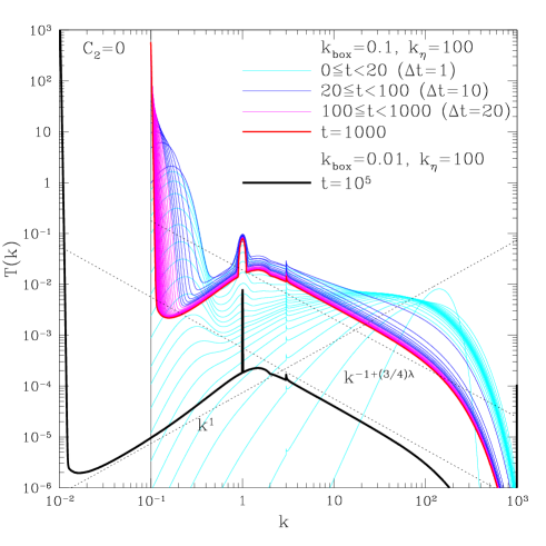
Figure 2: Evolution of normalized spectrum $T(t,k)/E(t)$ for $k_{\text{box}}=0.1$. The initial spectrum was $T(0,k)=k^{4}\exp[-(k/k_{\eta})^{2}]$. The long-term solution for $k_{\text{box}}=0.01$ is also shown. Spectra at $k<1$ are steeper than $k^{1}$ due to higher-order corrections: they can be well fitted by polynomials in the form $k+ak^{2}+\dots$ [Eq. (22)]. The blip at $k=3$ is the point where the solutions of Eq. (8) at $k<3$ and of Eq. (4) at $k>3$ are spliced together. This device allows us to achieve higher Pe. We have checked that moving around the splicing wave number or solving the full integral equation in the entire domain (at lower Pe) do not change the solution.

III.4 Case of $C_{2}=0$

When the Corrsin invariant is zero, the theory developed above has to be modified somewhat. The dominant term in the small-$k$ solution is $\sim k^{4}$ and includes contributions both from the initial spectrum and from the initial finite amount of nonlinear transfer of scalar variance from the flow-scale mode: Equation (12) is replaced by

$$T(t,k) = \left[C_{4}+\Phi(t,k)\right]k^{4}e^{-k^{2}t},$$ (23)

$$\Phi(t,k) = {3\over 4}\int_{0}^{t}\hskip-2.84526ptdt^{\prime}e^{k^{2}t^{\prime}}\hskip-2.84526pt\int_{-1}^{1}\hskip-2.84526ptdz(1-z^{2})T(t^{\prime},1+kz).\quad$$ (24)

In the transient stage ($1\ll t\ll 1/k_{\text{box}}^{2}$), we have, at $k\ll 1/\sqrt{t}$, $\Phi(t,k)\simeq\int_{0}^{t}dt^{\prime}T_{1}(t^{\prime})\to\text{const}$ as long as $T_{1}(t)$ decays faster than $1/t$ [cf. Eq. (14)]. Since $\Phi(t,k)$ also remains finite for $k\sim 1/\sqrt{t}$, we can estimate the flow scale modes $T(t,1+q)$ by substituting the solution (23) into Eq. (11) and assuming that $\Phi(t,k)$ is approximately constant at the values of $k$ that matter. This will produce errors of order unity in the prefactors but yield correct scalings and asymptotic decay laws. Note that because the nonlinear-transfer contribution is $\sim k^{4}$, the higher-order terms in the Taylor expansion for the initial spectrum do not affect the asymptotic solutions.

Further derivation for the $C_{2}=0$ case follows the same general scheme as the theory for $C_{2}>0$. In the transient stage, Eq. (13) is replaced by

$$T(t,1+q)\sim{2+q^{2}t\over t^{3}}\,e^{-q^{2}t},$$ (25)

where we have dropped prefactors of order unity. Note that the transient-stage decay of the flow-scale peak, $T_{1}(t)\sim 1/t^{3}$, is faster then for the $C_{2}>0$. This is the only important change that results from the vanishing of $C_{2}$. The intermediate asymptotic ($1/\sqrt{t}\ll k\ll 1$) is again $T(t,k)\sim T_{1}(t)t^{-1/2}k$ [cf. Eq. (15)]. In the long-time limit, Eq. (16) is replaced by

$$T(t,1+q)\sim{k_{\text{box}}^{2}\over t}\,(k_{\text{box}}^{2}-q^{2})\,e^{-k_{\text{box}}^{2}t},$$ (26)

the box mode decays according to [cf. Eq. (17)]

$$T(t,k_{\text{box}})\sim k_{\text{box}}^{4}e^{-k_{\text{box}}^{2}t}\left[C_{4}+O(k_{\text{box}}^{4}\ln t)\right],$$ (27)

and the intermediate asymptotic at $k_{\text{box}}\ll k\ll 1$ is $T(t,k)\sim T_{1}(t)k_{\text{box}}k$ [cf. Eq. (19)].

The developments for the nonsingular spectrum and for the total scalar variance are exactly as described in Sec. III.2 and Sec. III.3. The only change is in the transient-stage decay laws due to faster decay of the flow-scale mode [Eq. (25)]: the contribution to the scalar variance from the flow scale and the nonsingular spectrum is $\sim 1/t^{7/2}$; the contribution from the small-$k$ peak is $\sim 1/t^{5/2}$. The latter dominates and, therefore, determines the decay law for the total variance. The behavior in the long-time limit is the same as for $C_{2}>0$.

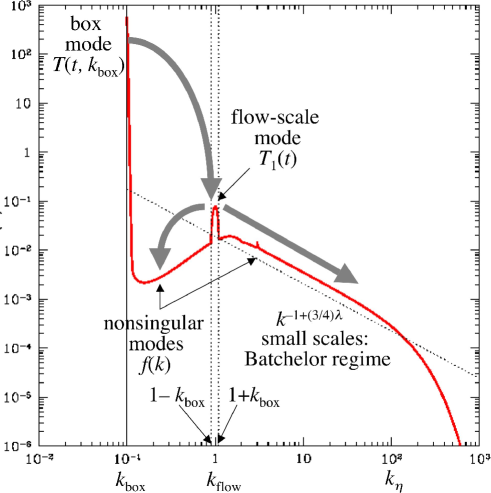
Figure 3: Structure of the “strange mode.” The spectrum is from a run with $k_{\text{box}}=0.1$, $k_{\eta}=100$ (the same as in Fig. 2, $t=1000$). Gray arrows show directions of couplings (transfer of scalar variance).

III.5 Numerical solution

We have checked our analytical solution by solving Eq. (8) numerically. The powerlike decay laws for the flow-scale mode $T(t,1)$ and for the total variance are in good agreement with theory, but they can only can be seen if the scale separation between the box and the flow is sufficiently large [$k_{\text{box}}\sim 0.01$; see Fig. 1(a)]. Spectra (Fig. 2) and long-term decay rates [Fig. 1(b)] are clearly in agreement with theory already at moderate scale separations. A simple way to estimate the threshold at which the decay rate ceases to be determined by box-scale diffusion is by requiring that the box decay rate should be smaller than the Lagrangian-stretching value: $\lambda=(40/9)k_{\text{box}}^{2}<1$, so $k_{\text{box}}\lesssim 0.47$. Consistent with this estimate, the box value still works for $k_{\text{box}}=1/3$ [Fig. 1(b); cf. Haynes and Vanneste (2005)]. Obviously, Eq. (8) itself with the cutoff at $k_{\text{box}}$ is only technically valid when $k_{\text{box}}\ll 1$, but we see that it continues to yield reasonable solutions even at moderate $k_{\text{box}}$.

IV Discussion

We now have a physical picture of the “strange mode”: the small-$k$ peak (singularity at the box scale) serves as a slowly decaying source to the flow-scale mode (singularity at $k=1$), which, in turn, is mixed by the random flow and thus excites the nonsingular modes at small [Eq. (5)] and large [Eq. (22)] scales. The structure of the spectrum is illustrated in Fig. 3.

The low-wave-number behavior of the decaying scalar field was previously analyzed in a heuristic way by Kerstein and McMurtry Kerstein and McMurtry (1994) (see also Gonzalez (2002) for a treatment based on one of the turbulence closure schemes, which gives mostly similar results). They considered advection by a narrow-band (i.e., single-scale) forced random flow in an unbounded domain — i.e., in the regime that we call the transient (powerlike-decay) stage. They recognized the defining role of coupling between the large scales ($k\lesssim k_{\text{peak}}$) and the flow scale ($k=k_{\text{flow}}=1$) and derived the $k^{4}$ scaling at $k\ll k_{\text{peak}}$ with a exponential fall off at $k>k_{\text{peak}}$ [Eq. (12)] and the ensuing powerlike-decay laws for the case of $C_{2}=0$ (see the end of Sec. III.4). For the intermediate rage $k_{\text{peak}}\ll k\ll 1$, they predicted a $k^{2}$ spectrum (in 3D) — in contrast to our $k^{1}$ result [Eqs. (15) and (22) and Sec. III.4]. The reason for the discrepancy is as follows. The analysis of Kerstein and McMurtry (1994) is based on Taylor-expanding the flow around $k=1$ — i.e., in terms of our theory — setting $T(t,1+q)\simeq T(t,1)$ in Eq. (9), which gives $S(t,k)\simeq k^{4}T(t,1)$. If we had used the resulting equation to solve for $T(t,k)$ at $k_{\text{peak}}\ll k\ll 1$, we would also have obtained $T(t,k)\sim k^{2}$. However, as we have seen above, the width of the flow-scale singularity is $\sim k_{\text{peak}}$ [Eqs. (13) and (25)], so Taylor expansion cannot be used in Eq. (9) for $k\gg k_{\text{peak}}$. In this intermediate range, the integral in Eq. (9) must instead be replaced by the integral over the entire flow-scale peak, resulting in our $k^{1}$ scaling. The $k^{2}$ term enters as a correction due to the interaction between nonsingular modes [Eq. (22)].

Finally, let us comment on our modeling assumptions. The white-noise approximation might appear drastic: the correlation time of any realistic flow is comparable to the flow time scale $\sim(uk_{\text{flow}})^{-1}\sim\kappa_{2}^{-1}$. However, since the scalar decay time is much longer than the flow time scale (provided $k_{\text{box}}\ll k_{\text{flow}}$), the white-noise model appears reasonable. We believe it also correctly captures the small-scale structure: the key factor here is the statistics of fluid displacements, which are integrals of velocity and are finite-time correlated even for a white-in-time velocity.

Our model flow was single scale. Although such flows can be set up in the laboratory Rothstein et al. (1999); Voth et al. (2003) , the real-world mixing problems usually contain (at sufficiently small scales) a wide (inertial) scale range of three-dimensional turbulent motions. While the variance spectrum in the inertial range should follow the Obukhov-Corrsin $k^{-5/3}$ law Obukhov (1949); Corrsin (1951b) and there will be another transient powerlike-decay stage Corrsin (1951a); Chasnov (1994); Eyink and Xin (2000); Chaves et al. (2001); Chertkov and Lebedev (2003), the long-term decay (after the scalar variance reaches $k<k_{\text{flow}}$) should still be qualitatively described by our theory. Another modification that results from the relaxation of the single-scale assumption concerns the intermediate wave-number range $k_{\text{peak}}\ll k\ll k_{\text{flow}}$. As noted in Kerstein and McMurtry (1994) and confirmed in pipe-flow mixing experiments Guilkey et al. (1997), the interaction between the $k=k_{\text{peak}}$ mode and the low-wave-number tail of the kinetic-energy spectrum ($\sim k^{4}$) can change the scaling of the scalar-variance spectrum in this range.

In conclusion, we emphasize that, in any laboratory experiment aiming to test our results, the stirring must be done at scales substantially smaller than the system size to ensure that $k_{\text{box}}\ll k_{\text{flow}}$. It was just such a set up (in 2D) that allowed Voth et al. Voth et al. (2003) to show experimentally that the global mixing rate was much smaller than that predicted by the Lagrangian-stretching theories and consistent with the box-scale turbulent-diffusion rate — precisely the point the theory presented above is meant to demonstrate.