Anisotropy in Turbulent Flows and in Turbulent Transport

Abstract

The problem of anisotropy and its effects on the statistical theory of high Reynolds-number (Re) turbulence (and turbulent transport) is intimately related and intermingled with the problem of the universality of the (anomalous) scaling exponents of structure functions. Both problems had seen tremendous progress in the last five years. In this review we present a detailed description of the new tools that allow effective data analysis and systematic theoretical studies such as to separate isotropic from anisotropic aspects of turbulent statistical fluctuations. Employing the invariance of the equations of fluid mechanics to all rotations, we show how to decompose the (tensorial) statistical objects in terms of the irreducible representation of the SO($d$) symmetry group (with $d$ being the dimension, $d=2$ or 3). This device allows a discussion of the scaling properties of the statistical objects in well defined sectors of the symmetry group, each of which is determined by the “angular momenta” sector numbers $(j,m)$. For the case of turbulent advection of passive scalar or vector fields, this decomposition allows rigorous statements to be made: (i) the scaling exponents are universal, (ii) the isotropic scaling exponents are always leading, (iii) the anisotropic scaling exponents form a discrete spectrum which is strictly increasing as a function of $j$. This emerging picture offers a complete understanding of the decay of anisotropy upon going to smaller and smaller scales. Next we explain how to apply the SO(3) decomposition to the statistical Navier-Stokes theory. We show how to extract information about the scaling behavior in the isotropic sector. Doing so furnishes a systematic way to assess the universality of the scaling exponents in this sector, clarifying the anisotropic origin of the many measurements that claimed the opposite. A systematic analysis of Direct Numerical Simulations (DNS) of the Navier-Stokes equations and of experiments provides a strong support to the proposition that also for the non-linear problem there exists foliation of the statistical theory into sectors of the symmetry group. The exponents appear universal in each sector, and again strictly increasing as a function of $j$. An approximate calculation of the anisotropic exponents based on a closure theory is reviewed. The conflicting experimental measurements on the decay of anisotropy are explained and systematized, showing agreement with the theory presented here.

1 Introduction

The statistical theory of fluid turbulence is concerned with correlation functions of the turbulent velocity vector field $\mbox{\boldmath$u$}(\mbox{\boldmath$x$},t)$ where $x$ is the spatial position and $t$ the time [1]. Since the velocity field is a vector, multi-point and multi-time correlation functions are in general tensor functions of the vector positions and the scalar times. Naturally such functions have rather complicated forms which are difficult to measure and to compute. Consequently, almost from its very beginning, the statistical theory of turbulence was discussed in the context of an isotropic and homogeneous model. The notion of isotropic turbulence was first introduced by G. I. Taylor in 1935 [2]. It refers to a turbulent flow, in which the statistical averages of every function of the velocity field and its derivatives with respect to a particular frame of axes is invariant to any rotation in the axes. This is a very effective mathematical simplification which, if properly used, can drastically reduce the mathematical complexity of the theory. For this reason, it was very soon adopted by others, such as T. D. Kármán and L. Howarth [3] who derived the Kármán-Howarth equation (see below), and A. N. Kolmogorov [4, 5] who derived the 4/5 law (re-derived below). In fact, most of the theoretical work in turbulence in the past sixty years was limited to the isotropic model.

Experimentally, however, we know that isotropy holds only as an approximation with a varying degree of justification. In all realistic flows there always exists some anisotropy at all scales; the statistical properties of the velocity field are effected by the geometry of the boundaries or the driving mechanism, which are never rotationally invariant [6, 7, 8, 9, 10, 11, 12, 13, 14]. Therefore, a realistic description of turbulence cannot be purely isotropic and must contain some anisotropic elements. Yet the problem is that once we take anisotropy into account, we face a drastic increase in the complexity of the theory. The number of variables that is needed to describe the common statistical quantities, such as correlation functions and structure functions of the velocity field, increases a lot. For example, under shear there is a characteristic length scale, which can be constructed from the typical velocity and the typical shear [8, 15]. This length has to be considered in order to distinguish those scales where the turbulent evolution is mainly dominated by the inertial effects of fluid mechanics or by the direct input of energy due to the anisotropic shear [16, 17, 18, 19]. Similarly, all dimensional estimates acquire a significant degree of ambiguity because of the proliferation of different dimensional quantities related to the parameters of anisotropy. As a consequence of these inherent difficulties the existing anisotropic effects were simply ignored in many of the experimental and simulational studies of statistical turbulence. This attitude gave rise to ambiguous assessments of important fundamental issues like the universality of the scaling exponents in turbulence.

The standard justification for ignoring anisotropic effects is that the basic phenomenology, since the pioneering works of Kolmogorov [4, 5], predicts a recovery of isotropy at sufficiently small scales of the turbulent flows. Nevertheless, both recent experimental works and theoretical analysis suggested that the actual rate of recovery is much slower than predicted by simple dimensional analysis, pointing out even the possibility that some anisotropic correlation function, based on velocity gradients, stays $O(1)$ for any Re [20, 21, 7, 22]. In order to settle this kind of problems, theoretically or experimentally, it is crucial to possess systematic tools to disentangle isotropic from anisotropic fluctuations and to distinguish among different kinds of anisotropic fluctuations. Thus a central challenge in the theory of anisotropy in turbulence is the construction of an efficient mathematical language to describe it. Without a proper description, the complexities of the formalism can soon obscure the physical content of the processes that we wish to study.

The problem of anisotropy is not disconnected from the other fundamental problem which has to do with the nature of universality in turbulence. By universality, we mean the tendency of different turbulent systems to show the same small-scales statistical behavior when the measurements are done far away from the boundaries. Consider, for example, the longitudinal two-point structure function

$$S^{(2)}(\mbox{\boldmath$r$})\equiv\left<\delta u_{\ell}^{2}(\mbox{\boldmath$x$},\mbox{\boldmath$r$},t)\right>\ ,\quad\delta u_{\ell}(\mbox{\boldmath$x$},\mbox{\boldmath$r$},t)\equiv\hat{\mbox{\boldmath$r$}}\cdot\big{[}\mbox{\boldmath$u$}(\mbox{\boldmath$x$}+\mbox{\boldmath$r$},t)-\mbox{\boldmath$u$}(\mbox{\boldmath$x$},t)\big{]}\ ,$$ (1)

with $\hat{\mbox{\boldmath$r$}}$ being the unit vector in the direction of $r$, and $\left<\cdot\right>$ stands for an appropriate ensemble average. This function shows essentially the same dependence on the separation vector $r$, whether it is measured in the atmospheric boundary layer, in a wind tunnel or in a DNS, provided it is measured for sufficiently small separations and far from the boundaries. This high-degree of universality cannot be expected if anisotropic fluctuations were the dominant contributions to the two-point structure functions. Different boundary conditions and different forcing mechanism necessarily introduce different large-scale anisotropies in the flow, which would translate to different small-scale anisotropic fluctuations. Small-scale universality can be achieved only if anisotropic fluctuations are sub-leading with respect to the isotropic fluctuations. In the following, we also discuss which aspects of the anisotropic fluctuations are universal and which are not. We will see that some aspects of the anisotropic fluctuations depend on the boundary conditions while other aspects do not. In fact we will show that scaling exponents are expected to be universal whereas amplitudes depend on the boundary conditions.

In the last 5 years, a tremendous progress in the understanding of the two aforementioned problems, i.e., finding a mathematical language that properly describes anisotropic turbulence and its universal properties has been achieved. Not surprisingly, the two problems are closely related, as it often happens in physics - a problem becomes considerably simpler if described in the proper mathematical language. The technical core of these recent achievements is the SO($3$) decomposition [23]. This tool enjoys the advantages of being mathematically simple, yet very powerful and systematic. By using it, many of the mathematical complexities of dealing with anisotropy in turbulence and in other hydrodynamic problems are greatly simplified. The principal idea is to represent the main statistical observables, such as structure functions and correlation functions, in terms of their projections on the different $(j,m)$ sectors of the group of rotations. It can be applied to all the statistical quantities in turbulence, creating a detailed profile of the effects of anisotropy. Additionally, and perhaps more importantly, the SO($3$) decomposition reveals some new universal properties of fully developed turbulence. It is expected that each sector of the SO($3$) group has its own universal exponents. In particular, it is shown that the exponents associated with the anisotropic sectors are larger than the isotropic exponents, in accordance with the isotropization of the statistics as smaller and smaller scales are observed.

As already mentioned, the SO($3$) decomposition is useful also to investigate isotropic and anisotropic fluctuations in other hydrodynamic problems. In particular we will focus on the case of scalar and vector quantities passively advected by a turbulent velocity field. In these cases, one may often elevate the phenomenological assumptions made for turbulent anisotropic fluctuations to the status of rigorous statements [24]. By using a systematic decomposition in different sectors of the SO($3$) group one may show that passive scalars, advected by stochastic self-similar Gaussian velocity fields, always possess isotropic leading small-scale fluctuations. Moreover, one may quantitatively distinguish among different kinds of anisotropies, assessing their rate of decay by going to smaller and smaller scales. It turns out that the rate of recovery of isotropy is typically much slower than expected on the basis of dimensional analysis. Moreover, all different anisotropic fluctuations decay in a self-similar way but with different rates; the scaling exponents being universal, while prefactors are non-universal [25]. The very same can be rigorously proved for the passive advection of vector-like quantities, as for the case of magnetic fields when the feedback on the velocity evolution due to the Lorentz force is neglected. There, the vector nature of the transported quantity leads to an even richer, and more complex, list of possible anisotropic fluctuations [26, 27]. Another important problem which we address in detail is the case of the passive advection of a vector-like incompressible quantity, i.e. a passive vector with pressure [28]. Although without any counterpart in nature, such a system is particularly interesting because it can be seen, for some aspects, as the closest linear approximation to the non-linear Navier-Stokes evolution. For example, it allows to study in a systematic way some problems connected to the convergence of integrals involving the pressure term. Similar technical problems arise also in the analysis of both isotropic and anisotropic multi-point velocity correlations in Navier-Stokes equations.

Of course, a significant part of this review will be devoted to applications of the theoretical and technical tools to physical experimental data [29, 10, 13, 30, 31, 32, 33] and numerical data sets [34, 35, 36, 15, 37, 38]. In order to exploit the entire potentiality of the SO($3$) decomposition one needs to measure the whole velocity field, $\mbox{\boldmath$u$}(\mbox{\boldmath$x$})$, in a 3 dimensional volume. This is because in order to disentangle different projections on different sectors one needs to integrate the given correlation function against the proper eigenfunction of the rotation group on the 3$d$ sphere of radius $r$. By doing that, the exact projection on each different sector of the SO($3$) decomposition is under control, with the only practical limitations for reaching highly anisotropic sectors being the lack of resolution of highly fluctuating angular properties. At the present stage of experimental capabilities the exact decomposition can be carried out explicitly only in data sets coming from DNS. Here the velocity field in the whole testing volume is available. For experimental data, the best way to exploit the SO($3$) decomposition is to either select observables with vanishing isotropic components, in order to focus directly on anisotropic sectors, or to perform a multi-sector analysis, i.e. to fit simultaneously the isotropic and anisotropic components.

The review is organized as follows. Sect. 2 offers a historical review of isotropic turbulence. We present a modern derivation of the exact results pertaining to the 3’rd order structure function and the celebrated 4/5 law. We review the standard theory for all correlation functions, and discuss the experimental difficulties with the isotropic theory. These difficulties included apparent persistence of anisotropies into the small scales for high Re, apparent location dependent scaling exponents etc. In Sect. 3 we review the history of attempts to deal with anisotropy. In Section 4, the technical basis of the SO($3$) decomposition is introduced focusing on the particular statistical problems of anisotropic fluctuations discussed in the previous section. Then, in Sect. 5 we switch to study exactly solvable hydrodynamic problems with emphasis on either those aspects peculiar to each different model and to those features in common with the non-linear Navier-Stokes case. Among the common aspects we cite the possibility to study in these models in full details the foliation of the equations of correlation functions in different anisotropic sectors; the universality of isotropic and anisotropic exponents; the hierarchical organization of exponents –leading to recovery of small-scales isotropy. At the end of this section we present closure results for two-point turbulent structure function in the anisotropic sectors $j=2,4,6$. In Sect. 6, the utility of this language is demonstrated by discussing experimental data in atmospheric boundary layer and on homogeneous-shear flows. In Sect. 7, we present the analysis of anisotropy in DNS of typical strongly anisotropic flows. Two cases are discussed in depth: channel flows and random Kolmogorov flows, the latter being homogeneous flows stirred at the large scales. Sect. 8 presents a summary and conclusions. Technical details are collected in the appendices.

2 Historical Review: Isotropic Turbulence

In the first two sections we present a historical review. We start with the model of homogeneous isotropic turbulence, and then turn to previous attempts to treat theoretically anisotropy in turbulence.

2.1 Homogeneous and Isotropic Turbulence

The Navier-Stokes equations for the velocity field are invariant to all rotations:

$$\frac{\partial\mbox{\boldmath$u$}(\mbox{\boldmath$x$},t)}{\partial t}+\left[\mbox{\boldmath$u$}(\mbox{\boldmath$x$},t)\cdot\mbox{\boldmath$\nabla$}\right]\mbox{\boldmath$u$}(\mbox{\boldmath$x$},t) = -\mbox{\boldmath$\nabla$}p(\mbox{\boldmath$x$},t)+\nu\Delta^{2}\mbox{\boldmath$u$}(\mbox{\boldmath$x$},t)\ ,$$ (2)

$$\mbox{\boldmath$\nabla$}\cdot\mbox{\boldmath$u$}(\mbox{\boldmath$x$},t) = 0,$$

with $p(\mbox{\boldmath$x$},t)$ and $\nu$ being the pressure and kinematic viscosity respectively. Since the gradient and Laplacian operators are both rotationally invariant, the rotation symmetry of the equation can be broken only by anisotropic forcing terms or anisotropic boundary conditions. Rather naturally then the statistical theory of turbulence was mostly developed in the framework of isotropic turbulence [2]. The central idea of this approximation is that the statistical average of any function of the velocity components in any coordinate system is unaltered if this coordinate system is rotated or reflected in any manner. The assumption of isotropy was widely adopted. In 1938, Kármán and Howarth [3] used it to explore the second- and third-order correlation-functions of the velocity field. Their use of tensor notation was more elegant and compact than that used by Taylor. It enabled them to derive some constraints on these correlation functions and express them in terms of a few scalar functions. For example, for the second-order correlation-function in homogeneous turbulence

$$C^{\alpha\beta}(\mbox{\boldmath$r$},t)\equiv\left<u^{\alpha}(\mbox{\boldmath$x$}+\mbox{\boldmath$r$},t)u^{\beta}(\mbox{\boldmath$x$},t)\right>\ ,$$ (3)

they used the representation

$$C^{\alpha\beta}(\mbox{\boldmath$r$},t)=[f(r,t)-g(r,t)]\hat{r}^{\alpha}\hat{r}^{\beta}+g(r,t)\delta^{\alpha\beta}\ ,$$ (4)

and then derived a linear differential relation between $f(r,t)$ and $g(r,t)$ using the solenoidal condition of $\partial_{\alpha}C^{\alpha\beta}(\mbox{\boldmath$r$},t)=0$,

$$2f(r,t)-2g(r,t)=-r\frac{\partial f(r,t)}{\partial r}\ .$$

This means that under the assumption of isotropy, and using the solenoidal condition, the second-order correlation-function can be written in terms of one scalar function instead of nine. Similarly, Kármán and Howarth analyzed the third-order correlation function by representing it as an isotropic tensor and then reducing the number of scalar functions using the solenoidal condition. They were also able to connect it to the second-order correlation function in decaying turbulence using the Navier-Stokes equations. These computations have since found their way into every standard text-book on the statistical theory of turbulence.

The mathematical representation of isotropic turbulence has reached its most elegant and powerful form in a paper by H. P. Robertson from 1940 [39]. Robertson provided a systematic way to represent isotropic tensors using the theory of invariants. For example, to derive the general representation (4) in the stationary case using Robertson’s method, we consider the scalar function

$$C(\mbox{\boldmath$a$},\mbox{\boldmath$b$},\mbox{\boldmath$r$})\equiv C^{\alpha\beta}(\mbox{\boldmath$r$})a_{\alpha}b_{\beta}\ ,$$

with $a$ and $b$ being two arbitrary vectors. If $C^{\alpha\beta}(\mbox{\boldmath$r$})$ were an isotropic tensor, $C(\mbox{\boldmath$a$},\mbox{\boldmath$b$},\mbox{\boldmath$r$})$ would preserve its functional form upon an arbitrary (simultaneous) rotation of the three vectors $\mbox{\boldmath$r$},\mbox{\boldmath$a$},\mbox{\boldmath$b$}$. Using invariant theory, Robertson deduced that $C(\mbox{\boldmath$a$},\mbox{\boldmath$b$},\mbox{\boldmath$r$})$ must be a function of the six possible scalar products $(\mbox{\boldmath$r$}\cdot\mbox{\boldmath$r$})$, $(\mbox{\boldmath$r$}\cdot\mbox{\boldmath$a$})$,… and of the determinant $[\mbox{\boldmath$r$}\mbox{\boldmath$a$}\mbox{\boldmath$b$}]\equiv\epsilon_{\mu\alpha\beta}r^{\mu}a^{\alpha}b^{\beta}$. Additionally, by definition, it must be a bilinear function of $a$ and $b$ and therefore must have the following form:

$$C(\mbox{\boldmath$a$},\mbox{\boldmath$b$},\mbox{\boldmath$r$})=A(r)(\mbox{\boldmath$r$}\cdot\mbox{\boldmath$a$})(\mbox{\boldmath$r$}\cdot\mbox{\boldmath$b$})+B(r)(\mbox{\boldmath$a$}\cdot\mbox{\boldmath$b$})+C(r)[\mbox{\boldmath$r$}\mbox{\boldmath$a$}\mbox{\boldmath$b$}]\ ,$$

where $A(r)$, $B(r)$ and $C(r)$ are arbitrary functions. Finally, recalling that $C(\mbox{\boldmath$a$},\mbox{\boldmath$b$},\mbox{\boldmath$r$})$ is the contraction of $C^{\alpha\beta}(\mbox{\boldmath$r$})$ with $a$ and $b$, we find that

$$C^{\alpha\beta}(\mbox{\boldmath$r$})=A(r)r^{\alpha}r^{\beta}+B(r)\delta^{\alpha\beta}+C(r)\epsilon^{\mu\alpha\beta}r_{\mu}\ .$$

If we further demand $C^{\alpha\beta}(\mbox{\boldmath$r$})$ to be invariant to improper rotations as well (i.e., rotations plus reflections), we can drop the skew-symmetric part $\epsilon^{\mu\alpha\beta}$, thus retaining a representation which is equivalent to Eq. (4).

2.2 The 4/5 law in Isotropic Turbulence and its Generalization

By using the isotropic representation of the third-order correlation function, in 1941 Kolmogorov proved the “four-fifth law” well inside the inertial range of a fully developed turbulence. This law pertains to the third order moment of longitudinal velocity differences, stating that in homogeneous, isotropic and stationary turbulence, in the limit of vanishing kinematic viscosity $\nu\to 0$

$$\left<[\delta u_{l}(\mbox{\boldmath$x$},\mbox{\boldmath$r$},t)]^{3}\right>=-\frac{4}{5}\bar{\epsilon}r\ ,$$

where $\bar{\epsilon}$ is the mean energy flux per unit time and mass, $\bar{\epsilon}\equiv\nu\left<|\nabla_{\alpha}u_{\beta}|^{2}\right>$. The fundamental assumption needed to derive this law is the so-called “dissipation anomaly” which means that the dissipation is finite in the limit $\nu\to 0$. As noted in [5], “this is one of the most important results in fully developed turbulence because it is both exact and nontrivial. It thus constitutes a kind of ‘boundary condition’ on theories of turbulence: such theories, to be acceptable, must either satisfy the four-fifth law, or explicitly violate the assumptions made in deriving it”.

To demonstrate how isotropy helps in deriving this result, we present a re-derivation in which we will obtain an additional exact relation that appears to have the same status as the four-fifth law, pertaining to homogeneous, stationary and isotropic turbulence with helicity [40, 41]. Defining the velocity $\mbox{\boldmath$v$}(\mbox{\boldmath$x$},t)$ as $\mbox{\boldmath$v$}(\mbox{\boldmath$x$},t)\equiv\mbox{\boldmath$u$}(\mbox{\boldmath$x$},t)-\left<\mbox{\boldmath$u$}\right>$ we consider the simultaneous 3rd order tensor correlation function which depends on two space points:

$$J^{\alpha,\beta\gamma}(\mbox{\boldmath$r$})\equiv\left<v^{\alpha}(\mbox{\boldmath$x$}+\mbox{\boldmath$r$},t)v^{\beta}(\mbox{\boldmath$x$},t)v^{\gamma}(\mbox{\boldmath$x$},t)\right>\ .$$ (5)

We show that in the limit $\nu\to 0$, under the same assumption leading to the fourth-fifth law, this correlation function reads [41]

$$J^{\alpha,\beta\gamma}(\mbox{\boldmath$r$})=-{\bar{\epsilon}\over 10}(r^{\gamma}\delta_{\alpha\beta}+r^{\beta}\delta_{\alpha\gamma}-{2\over 3}r^{\alpha}\delta_{\beta\gamma})-{h\over 30}(\epsilon_{\alpha\beta\delta}r^{\gamma}+\epsilon_{\alpha\gamma\delta}r^{\beta})r^{\delta}\ ,$$ (6)

where $\delta_{\alpha\beta}$ is the Kronecker delta and $\epsilon_{\alpha\beta\gamma}$ is the fully antisymmetric tensor. The quantity $h$ is the mean dissipation of helicity per unit mass and time,

$$h\equiv\nu\left<(\nabla^{\alpha}u^{\beta})(\nabla^{\alpha}[\mbox{\boldmath$\nabla$}\times\mbox{\boldmath$u$}]^{\beta})\right>\ ,$$

where repeated indices are summed upon. In the derivation below it assumed that $h$ remains constant when $\nu\rightarrow 0$ in the same spirit of the dissipation anomaly [42, 43, 44]. The first term in Eq. (6) is just the 4/5 law. The new part of result (6) can be also displayed in a form that depends on $h$ alone by introducing the longitudinal and transverse parts of $u$: the longitudinal part is $\mbox{\boldmath$u$}_{l}\equiv\mbox{\boldmath$r$}(\mbox{\boldmath$u$}\cdot\mbox{\boldmath$r$})/r^{2}$ and the transverse part is $\mbox{\boldmath$u$}_{t}\equiv\mbox{\boldmath$u$}-\mbox{\boldmath$u$}_{l}$. In terms of these quantities we can present a “two fifteenth law”

$$\left<[\delta\mbox{\boldmath$u$}_{l}(\mbox{\boldmath$x$},\mbox{\boldmath$r$},t)]\cdot[\mbox{\boldmath$u$}_{t}(\mbox{\boldmath$r$}+\mbox{\boldmath$x$},t)\times\mbox{\boldmath$u$}_{t}(\mbox{\boldmath$x$},t)]\right>=\frac{2}{15}hr^{2}\ .$$ (7)

We note that this result holds also when we replace $u$ by $v$ everywhere.

To derive the result (6) we start from the correlation function $J^{\alpha,\beta\gamma}(\mbox{\boldmath$r$})$ which is symmetric with respect to exchange of the indices $\beta$ and $\gamma$ as is clear from the definition. In an isotropic homogeneous medium with helicity (no inversion symmetry), the most general form of this object is [41]:

$$J^{\alpha,\beta\gamma}(\mbox{\boldmath$r$})=a_{1}(r)[\delta_{\alpha\beta}r^{\gamma}+\delta_{\alpha\gamma}r^{\beta}+\delta_{\beta\gamma}r^{\alpha}]+\tilde{a}_{1}(r)[\delta_{\alpha\beta}r^{\gamma}+\delta_{l}{\alpha\gamma}r^{\beta}-2\delta_{\beta\gamma}r^{\alpha}]$$

$$+b_{2}(r)[\epsilon_{\alpha\beta\delta}r^{\gamma}+\epsilon_{\alpha\gamma\delta}r^{\beta}]r^{\delta}+a_{3}(r)[\delta_{\alpha\beta}r^{\gamma}+\delta_{\alpha\gamma}r^{\beta}+\delta_{\beta\gamma}r^{\alpha}-5r^{\alpha}r^{\beta}r^{\gamma}/r^{2}]\ .$$

This general representation is invariant to the choice of orientation of the coordinates. Not all the coefficients are independent for incompressible flows. Requiring $\partial J^{\alpha,\beta\gamma}(\mbox{\boldmath$r$})/\partial r^{\alpha}=0$ leads to two relations among the coefficients:

$$\Big{(}{d\over dr}+{5\over r}\Big{)}a_{3}(r)={2\over 3}{d\over dr}\big{[}a_{1}(r)+\tilde{a}_{1}(r)\big{]}\ ,\qquad\Big{(}{d\over dr}+{3\over r}\Big{)}\big{[}5a_{1}(r)-4\tilde{a}_{1}(r)\big{]}=0\ .$$

As we have two conditions relating the three coefficients $a_{1},\tilde{a}_{1}$ and $a_{3}$ only one of them is independent. Kolmogorov’s derivation related the rate of energy dissipation to the value of the remaining unknown. Here the coefficient $b_{2}$ remains undetermined by the incompressibility constraint; it will be determined by the rate of helicity dissipation.

Kolmogorov’s derivation can be paraphrased in a simple manner. Begin with the second order structure function $\tilde{S}^{(2)}(r)\equiv\langle|\mbox{\boldmath$u$}(\mbox{\boldmath$x$}+\mbox{\boldmath$r$})-\mbox{\boldmath$u$}(\mbox{\boldmath$x$})|^{2}\rangle$. Computing the rate of change of this (time-independent) function from the Navier-Stokes equations (2) we find

$$0={\partial\tilde{S}^{(2)}(r)\over 2\partial t}=-{\mathcal{D}}^{(2)}(r)-2\bar{\epsilon}+\nu\nabla^{2}\tilde{S}^{(2)}(r)\ ,$$ (8)

where ${\mathcal{D}}^{(2)}(r)$ stems from the nonlinear term $(\mbox{\boldmath$u$}\cdot\mbox{\boldmath$\nabla$})\mbox{\boldmath$u$}$ and as a result it consists of a correlation function including a velocity derivative. The conservation of energy allows the derivative to be taken outside the correlation function:

$${\mathcal{D}}^{(2)}(r)\equiv{\partial\over\partial r^{\beta}}\langle u^{\alpha}(\mbox{\boldmath$x$},t)u^{\alpha}(\mbox{\boldmath$x$}+\mbox{\boldmath$r$},t)\big{[}u^{\beta}(\mbox{\boldmath$x$},t)-\!u^{\beta}(\mbox{\boldmath$x$}+\mbox{\boldmath$r$},t)\big{]}\rangle\ .$$ (9)

In terms of the function of Eq. (5) we can write

$${\mathcal{D}}^{(2)}(r)={\partial\over\partial r^{\beta}}\Big{[}J^{\alpha,\beta\alpha}(\mbox{\boldmath$r$},t)-J^{\alpha,\beta\alpha}(-\mbox{\boldmath$r$},t)\Big{]}\ .$$ (10)

Note that Eq. (5) is written in terms of $v$ rather than $u$, but using the incompressibility constraint we can easily prove that Eq. (9) can also be identically written in terms of $v$ rather than $u$. We proceed using Eq. (2.2) in Eq. (10), and find

$${\mathcal{D}}^{(2)}(r)=2{\partial\over\partial r^{\beta}}r^{\beta}\big{[}5a_{1}(r)+2\tilde{a}_{1}(r)\big{]}\ .$$ (11)

For $r$ in the inertial interval, and for $\nu\to 0$, we can read from Eq. (8) ${\mathcal{D}}^{(2)}(r)=-2\bar{\epsilon}$ and therefore have the third relation that is needed to solve all the three unknown coefficients. A calculation leads to

$$a_{1}(r)=-2\bar{\epsilon}/45\ ,\quad\tilde{a}_{1}=-\bar{\epsilon}/18\ ,\quad a_{3}=0\ .$$

The choice of the structure function $\tilde{S}_{2}(r)$ leaves the coefficient $b_{2}(r)$ undetermined, and another correlation function is needed in order to remedy the situation. Since the helicity is $\mbox{\boldmath$u$}\cdot[\mbox{\boldmath$\nabla$}\times\mbox{\boldmath$u$}]$, we seek a correlation function which is related to the helicity of eddys of scale of $r$:

$$T^{(2)}(r)\equiv\langle\big{[}\mbox{\boldmath$u$}(\mbox{\boldmath$r$}+\mbox{\boldmath$x$},t)-\mbox{\boldmath$u$}(\mbox{\boldmath$x$},t)\big{]}\cdot\big{[}\mbox{\boldmath$\nabla$}\times\mbox{\boldmath$u$}(\mbox{\boldmath$x$}+\mbox{\boldmath$r$},t)-\mbox{\boldmath$\nabla$}\times\mbox{\boldmath$u$}(\mbox{\boldmath$x$},t)\big{]}\rangle\ .$$

Using the Navier-Stokes equations to compute the rate of change of this quantity we find

$$0={\partial T^{(2)}(r)\over 2\partial t}=-G^{(2)}(r)-2h-\nu\nabla^{2}T^{(2)}(r)\ ,$$ (12)

which is the analog of (8), and where

$$G^{(2)}(r) = \left\{\langle\mbox{\boldmath$u$}(\mbox{\boldmath$x$},t)\cdot\left[\mbox{\boldmath$\nabla$}_{r}\times\left[\mbox{\boldmath$u$}(\mbox{\boldmath$x$}+\mbox{\boldmath$r$},t)\times\left[\mbox{\boldmath$\nabla$}_{r}\times\mbox{\boldmath$u$}(\mbox{\boldmath$x$}+\mbox{\boldmath$r$},t)\right]\right]\right]\rangle\right\}$$ (13)

$$+ \{{\rm term}~{}\mbox{\boldmath$r$}\to-\mbox{\boldmath$r$}\}\ .$$

The conservation of helicity allows the extraction of two derivatives outside the correlation functions. The result can be expressed in terms of the definition (5):

$$G^{(2)}(r)={\partial\over\partial R^{\lambda}}{\partial\over\partial r^{\kappa}}\epsilon_{\alpha\lambda\mu}\epsilon_{\mu\beta\nu}\epsilon_{\nu\kappa\gamma}\big{[}J^{\alpha,\beta\gamma}(\mbox{\boldmath$r$})+J^{\alpha,\beta\gamma}(-\mbox{\boldmath$r$})\big{]}\ .$$

Substituting Eq. (2.2) we find

$$G^{(2)}(r)=2{\partial^{2}\over\partial r^{\lambda}\partial r^{\kappa}}b_{2}(r)\big{[}r^{\lambda}r^{\kappa}-\delta_{\lambda\kappa}r^{2}\big{]}\ ,$$

which is the analog of Eq. (11). Using Eq. (12) in the inertial interval in the limit $\nu\to 0$ we find the differential equation

$$r^{2}{d^{2}b_{2}(r)\over dr^{2}}+9r{db_{2}(r)\over dr}+15b_{2}(r)=-{h\over 2}\ .$$

The general solution of this equation is $b_{2}(r)=-h/30+\alpha_{1}r^{-5}+\alpha_{2}r^{-3}$. Requiring finite solutions in the limit $r\to 0$ means that $\alpha_{1}=\alpha_{2}=0$. Accordingly we end up with Eq. (6). The moral of this example is that even in isotropic and homogeneous systems there exist sub-leading terms which can become dominant for specially selected objects like (7). Once anisotropy exists, there are many more (in fact infinitely many) sub-leading contributions that need to be assessed carefully. Similar results for slightly different correlation functions have also been found in [45, 46]

2.3 Kolmogorov’s Theory for 2’nd, 4’th, and Higher Order Structure Functions

Unfortunately, the exact result pertaining to the 3’rd order structure function is rather unique. The moment we consider 2’nd, 4’th or higher order correlation functions there is no exact result for the scaling exponents. Kolmogorov’s 1941 theory states that, for Re large enough, small-scales turbulent fluctuations should recover isotropy and homogeneity (if measured far enough from boundaries) and should possess universal scaling properties depending only on the mean energy flux, $\bar{\epsilon}$. For homogeneous and isotropic ensembles one defines

$$S^{(n)}(r)\equiv\left<\delta u_{\ell}^{n}(\mbox{\boldmath$x$},\mbox{\boldmath$r$},t)\right>\ =(\bar{\epsilon}r)^{n\over 3}f^{(n)}({r\over L_{0}},{\eta\over r}),$$ (14)

where $L_{0}$ and $\eta$ are the integral length scale and the viscous scale, respectively. The function $f^{(n)}$ is supposed to be well behaved in the limit of infinite Reynolds numbers for fixed separation, $r$: $\lim_{x,y\rightarrow 0}f^{(n)}(x,y)=$ const. In this limit, the celebrated K41 scaling prediction for structure functions in the inertial range, $\eta\ll r\ll L_{0}$, follows:

$$S^{(n)}(r)\sim C^{(n)}(\bar{\epsilon}r)^{\zeta^{(n)}},\qquad\mbox{with}\;\;\zeta^{(n)}=\frac{n}{3}.$$ (15)

In (15) the constants $C^{(n)}$ depend only on the large scale properties. Because of stationarity, the mean energy flux in Eq. (15) can be equally taken to be the mean energy input or the mean energy dissipation.

Kolmogorov’s theory goes beyond the scaling prediction (15). For example, any non-vanishing $p$th order structure functions, including purely transversal and mixed longitudinal-transversal velocity increments, must possess the same scaling exponents:

$$S^{(n,m)}(r)\equiv\left<\delta u_{\ell}^{n}(\mbox{\boldmath$r$})\delta u_{t}^{m}(\mbox{\boldmath$r$})\right>\sim C^{(n,m)}(\bar{\epsilon}r)^{\frac{(n+m)}{3}},$$ (16)

where $p=n+m$, $\delta\mbox{\boldmath$u$}_{t}(\mbox{\boldmath$r$})\equiv\delta\mbox{\boldmath$u$}(\mbox{\boldmath$r$})-\delta u_{\ell}(\mbox{\boldmath$r$})\hat{\mbox{\boldmath$r$}}$, and $\delta u_{t}(\mbox{\boldmath$r$})$ is one of the components of the two-dimensional transverse velocity difference. Notice that due to the assumption of isotropy, only even combinations of transversal increment in (16) have a non vanishing average. It is also not difficult to extend the K41 reasonings to describe also correlation functions at the viscous scales, i.e. observables based on gradients statistics [47, 48].

2.4 Experimental Difficulties with the Isotropic Theory

On the whole, experimental tests of Kolmogorov’s theory ran into increasing difficulties when the data were analyzed with greater detail. The first systematic attempt to check the isotropic scaling (15) for high Re number turbulence was [49]. These authors performed a high statistical test of K41 theory by going beyond the usual two-point correlations. They measured structure functions of higher order, reaching good evidence that there exist anomalous deviations from the scaling exponents (15). Their data substantiate a power-law behavior with $\zeta(n)\neq n/3$. At that time, and for many year later, the situation was very controversial both theoretically and experimentally. There appeared many claims that the observed deviations were due to sub-leading finite-Reynolds effects. One should not underestimate the difficulties of getting reliable estimates of the scaling exponents. First, one must expect finite Reynolds numbers corrections which may strongly reduce the inertial range where scaling laws are expected or introduce anisotropic corrections to the isotropic K41 predictions. Both effects are usually present in all experiments and numerical simulations. Nowadays, state-of-the-art experiments of turbulence in controlled geometries reach a maximum Re numbers measured on the gradient scales, $\lambda^{-1}=\langle|\mbox{\boldmath$\nabla$}\mbox{\boldmath$u$}|\rangle/\langle|\mbox{\boldmath$u$}|\rangle$, of $R_{\lambda}\sim 5000$ where $R_{\lambda}=\frac{\lambda U}{\nu}$ and $U$ is the typical large scale velocity. In atmospheric flows $R_{\lambda}$ can be as high as $R_{\lambda}\sim 20000$ but at the expense of high anisotropy. More complex is the situation of DNS where the best resolution ever reached up to now is $4096^{3}$ [50], corresponding to a $R_{\lambda}\sim 1100$. DNS allow a minimization of the anisotropic corrections, by implementing periodic boundary conditions and fully isotropic forcing, something which is not experimentally feasible. However, also in DNS the discrete symmetries induced by the finite lattice-spacing do not allow for perfect isotropic statistics. We thus either have high-Reynolds-numbers experiments which are strongly perturbed by anisotropic effects, or DNS isotropic flow at moderate Reynolds numbers. Therefore, one has to face the problem of how to disentangle isotropic from anisotropic fluctuations and how to extract information on the asymptotic scaling with a finite –often short– inertial-range extension. Only recently, after many experimental and numerical confirmations of the results of [49], the situation became clearer [51]. We may affirm now with some degrees of certitude that the isotropic scaling exponents are anomalous, the K41 prediction $\zeta(n)=n/3$ is wrong, except for $n=3$ which is fixed to be $\zeta(3)=1$ by the exact $4/5$ law. Moreover, the possibility to show analytically the existence of anomalous scaling in turbulent advection [24], definitely eliminated those arguments supporting the impossibility to have a Re-independent anomalous scaling in any hydrodynamic system. From a phenomenological point of view, it is easy to extend the K41 theory such as to include anomalous scaling. Already Kolmogorov noticed, after Landau’s criticism in 1962, that it is unrealistic to expect the isotropic inertial range fluctuations to depend only on the mean energy dissipation, $\bar{\epsilon}$. Kolmogorov proposed in 1962 [52] to employ the coarse-grained energy dissipation over a box of size $r$,

$$\tilde{\epsilon}(r,\mbox{\boldmath$x$})={1\over r^{3}}\int_{|y|<r}d\mbox{\boldmath$y$}\bar{\epsilon}(\mbox{\boldmath$x$}+\mbox{\boldmath$y$}),$$ (17)

to match the correct dimensions of structure functions in (14), the so-called Refined Kolmogorov Hypothesis:

$$S^{(n)}(r)=C^{(n)}\langle\tilde{\epsilon}^{n\over 3}(r)\rangle r^{n\over 3}.$$ (18)

This hypothesis connects the deviation from the K41 prediction, $\zeta(n)-n/3=\tau(n/3)$, to the anomalous scaling of the coarse-grained energy dissipation : $\langle\tilde{\epsilon}^{n\over 3}(r)\rangle\sim r^{\tau(n/3)}$. Anomalous scaling of isotropic structure functions is therefore connected to the multifractal properties of the three dimensional energy dissipation field [5]. It should be noted however that the Refined Kolmogorov Hypothesis related inertial range scaling to scaling of dissipative quantities, and delicate issues connected to small distance expansions and fusion rules are being disregarded here [53, 54]. At any rate, the relation presented by Eq.(18) did not advance the calculation of the scaling exponents beyond crude phenomenology.

2.5 Persistence of Anisotropies

A central issue of K41 phenomenology is the assumption of return-to-isotropy for smaller and smaller scales. Recently this assumption had been put to test in experiments and simulations [21, 55, 10, 35]. A useful experimental set-up to test the return to isotropy is a homogeneous shear flow [6] where the large-scale mean-velocity has a linear profile: $\mbox{\boldmath$V$}=(V_{0}y,0,0)$. The shear is given by ${\mathcal{S}}_{ij}=\partial_{i}V_{j}=\delta_{iy}\delta_{jx}V_{0}$. We thus have a homogeneous but anisotropic flow, close to the ideal case for studying the influence of large scale anisotropies on the small scale statistics. “Small scales” are defined here in comparison to the characteristic shear length, $L_{\mathcal{S}}=\bar{\epsilon}^{1/3}/{\mathcal{S}}$; for $r\ll L_{\mathcal{S}}$ we may expect that anisotropic fluctuations are sub-leading with respect to the isotropic ones. The case $r\gg L_{\mathcal{S}}$ is of interest in situations where the shear is very intense, as very close to the walls in bounded flows. In such cases we expect a dramatic change from the K41 phenomenology [16, 18, 19]. Fortunately, it is not that difficult to design experiments or DNS possessing an almost perfect linear profile with homogeneous shear [21, 7, 55, 16]. A popular way to measure small-scales anisotropies is to focus on the Re dependence of isotropic and anisotropic statistical observables built in terms of velocity gradients. For example, due to the symmetries of the mean flow, gradients of the stream-wise component in the shear direction, $\partial_{y}u_{x}$, may have a skewed distribution only due to the anisotropic fluctuations; they have a symmetric PDF in a perfectly isotropic flow. A natural measure of the residual anisotropy at small scales as a function of Re is the mixed generalized skewness based on gradients:

$$M^{(2n+1)}(R_{\lambda})\frac{\langle(\partial_{y}u_{x})^{2n+1}\rangle}{\langle(\partial_{y}u_{x})^{2}\rangle^{\frac{2n+1}{2}}}.$$ (19)

These objects vanish in isotropic ensembles. Of course, at finite Reynolds numbers one expects that the large-scale anisotropy introduced by the shear still remains, even on the gradient scale. Therefore, the rate of decay of (19) as a function of Re is a quantitative indication of the rate of decay of anisotropy at small scales. In the next section we review Lumley’s dimensional arguments [8] for anisotropic fluctuations, which predicts:

$$M^{(2n+1)}(R_{\lambda})\sim R^{-{1\over 2}}_{\lambda},\qquad\forall\;\;n.$$ (20)

In fact, both numerical [21, 20] (at low Reynolds numbers) and experimental tests (up to $R_{\lambda}\sim 1000$) showed a clear disagreement with the dimensional prediction (20). For example in [7] the authors quote a decay in agreement with the prediction for $M^{(3)}(R_{\lambda})$, an almost constant behavior as a function of Re for the fifth order, $M^{(5)}(R_{\lambda})\sim O(1)$ and an increasing behavior for the seventh order $M^{(7)}(R_{\lambda})\sim R^{+0.63}_{\lambda}$ ! These results have cast a severe doubt on the fundamental assumption of the K41 theory. Similar results, with even more striking contradictions with the hypothesis of the return-to-isotropy, have been measured in the problem of passive scalar fluctuations, $\theta=T-\langle T\rangle$, advected by an isotropic velocity field in the presence of a mean homogeneous scalar gradient, $\mbox{\boldmath$\nabla$}\langle T\rangle=(g,0,0)$. The equation of motions for the passive advected field in this case are:

$$\partial_{t}\theta+\mbox{\boldmath$u$}\cdot\mbox{\boldmath$\nabla$}\theta=gu_{x}+\chi\partial^{2}\theta.$$

Both experimental and numerical data show a strong disagreement with the prediction that generalized skewness of temperature gradients becomes smaller upon increasing Reynolds and Peclet numbers [56, 57, 58, 59, 60, 61].

We will show below how the analysis based on SO(3) decomposition and its theoretical consequences settles this puzzle of strong persistence of anisotropies [35]. In fact, contrary to what appears, the K41 phenomenology with its assumption of return-to-isotropy and the above experimental results are not at all in contradiction (see section 6.2.1).

2.6 Longitudinal and Transversal Isotropic Structure Functions

Another debated issue concerning the K41 phenomenology and its multifractal generalization (18) has to do with the observed discrepancies between the scaling properties of longitudinal, transversal, and mixed longitudinal-transversal structure functions in (supposedly) isotropic fully developed turbulence [30, 62, 63, 64, 65]. As previously stated, K41 theory, for isotropic flows, predicts the same scaling behavior, in the limit of high Re, independent of the Cartesian components of the velocity increments in the structure functions. For a given order $p=m+n$ only prefactors in (16) may depend on the particular choice of $n$ and $m$. Let us denote with $\zeta^{(n,m)}$ the scaling exponent of the mixed structure function (16) made of $n$ longitudinal increments and of $m$ transversal increments in a isotropic ensemble:

$$S^{(n,m)}(r)\sim C^{(n,m)}r^{\zeta^{(n,m)}}.$$

For $p<4$ the issue does not exist; due to the incompressibility constraint all second and third order longitudinal or transversal structure functions have the same scaling in a isotropic ensemble. For $p>3$ many experiments and numerical simulations found that $\zeta^{(n,m)}<\zeta^{(n^{\prime},m^{\prime})}$ if $n<n^{\prime}$ and $m>m^{\prime}$ when $n+m=n^{\prime}+m^{\prime}$. It appears that with increasing $m$ the scaling exponents reduce (the signal is more intermittent). The largest difference for a structure function of order $p$ is therefore achieved when we compare the purely longitudinal scaling $\zeta(p,0)$ with the purely transversal scaling $\zeta(0,p)$. Other experimental data suggests the possibility of a slow tendency of the longitudinal and transversal scaling exponents to coalesce for increasing Re [66, 67, 68].

We will argue below that the experimental measurements of different exponents stems from anisotropic corrections that affect differently the longitudinal and transverse components. In other words, by not removing the anisotropic contributions, one cannot expect pure power-law behavior. The situation is more complex for the analysis of data from DNS. There, one may implement highly isotropic forcing and boundary conditions, such that in most cases any residual anisotropic effects may safely be neglected even at moderate Re numbers. On the other hand, state-of-the-art numerical simulations are still strongly limited in the maximum Re achievable. Only very recently reliable data with high-statistics became available at resolution $1024^{3}$ [64], while most of the previous DNS where limited to lower resolutions. At resolution of $1024^{3}$ one reaches a moderate $R_{\lambda}\sim 400$, far below many experiments. Because of the consequent limited extension of the inertial range, such DNS did not resolve the puzzle of longitudinal vs transversal scaling. The numerical results oscillate between evidence for different scaling properties and for its opposite [62, 64, 69, 70, 71]. The issue is complicated by the fact that longitudinal and transversal structure functions possess different finite Re effects. For example, in [64] it was shown that structure functions of different order have different dependence on the viscous cut-off; this introduces ambiguity in defining a common inertial range where power law is expected. We thus propose that until high resolution isotropic measurements became available, all evidence for different scaling exponents for longitudinal and transverse structure functions should be considered with suspicion.

2.7 Position Dependent Scaling Exponents

In some inhomogeneous simulations and experiments it was claimed that the measured scaling exponents depended on the point of measurement within the flow domain [72, 9, 18, 19, 73, 74]. If true, such finding would deal a death blow to the idea of universality of the scaling exponents in turbulence. It should be stressed that in all the examples where such findings were reported the flow contained strong anisotropic and inhomogeneous components and/or the scaling range was not sufficient to actually present direct log-log plots for the structure functions vs. $r$. In some of these cases, scaling was extracted by using the method called “Extended Self Similarity” (ESS) [51]; the use of this method can be dangerous in presence of anisotropic and inhomogeneous effects. Whenever strong anisotropies are present one has to distinguish among two scaling ranges. At scales larger than the shear length, the energy cascade mechanism of the Kolmogorov theory is overwhelmed by shearing effects [16, 19]. Only for scales smaller than the shear length the meaning of anisotropic corrections to the isotropic K41 scaling theory is well posed. We argue below that the reported position-dependent isotropic exponents in the latter case stem from anisotropic components which appear with different amplitudes at different points in the flow. The different “exponents” that were measured were not real exponents but the result of a crossover between the isotropic and anisotropic corrections. Once the data is projected onto the isotropic sector the leading exponents become position independent as expected.

3 Historical Review: Attempts at Anisotropy

3.1 Bachelor’s Approach

The first systematic approach to anisotropy in turbulence was suggested by G. K. Batchelor in 1946 [75]. Batchelor did not attempt to describe the most general form of anisotropy in turbulence, but instead confined himself to the easier case of axisymmetric turbulence. In axisymmetric turbulence the mean value of any function of the velocity field and its derivatives is invariant to all rotations of the axes in a given direction. Therefore, the anisotropy in axisymmetric turbulence is induced by a single direction in space. We denote this symmetry axis by the unit vector $n$. Being the easiest case of anisotropic turbulence, axisymmetric turbulence was the main model for studying anisotropy in subsequent years.

Batchelor used the invariant theory in order to take the anisotropy vector $n$ into account in the tensor representations. His method is simple: add the vector $n$ to the list of vectors in Robertson’s method. For example, suppose we wish to construct an axisymmetric representation of the second-order correlation function $C^{\alpha\beta}(\mbox{\boldmath$r$})$ defined in (3). Then, just as in the isotropic case, we create a scalar function by contracting the two indices of $C^{\alpha\beta}(\mbox{\boldmath$r$})$ with two arbitrary vector $a$ and $b$, with the difference that now we assume that the resultant scalar function depends on the unit vector $n$ as well as on the other vectors $r$, $a$ and $b$. We therefore look for an invariant representation of the scalar function $C(\mbox{\boldmath$r$},\mbox{\boldmath$n$},\mbox{\boldmath$a$},\mbox{\boldmath$b$})$, which depends only on the different scalar products $\mbox{\boldmath$r$}\cdot\mbox{\boldmath$r$}$, $\mbox{\boldmath$r$}\cdot\mbox{\boldmath$n$}$, $\mbox{\boldmath$r$}\cdot\mbox{\boldmath$a$}\$,… and the various determinants $[\mbox{\boldmath$r$}\mbox{\boldmath$n$}\mbox{\boldmath$a$}]$, $[\mbox{\boldmath$r$}\mbox{\boldmath$n$}\mbox{\boldmath$b$}]\$,… For some reason, Batchelor decided to ignore the skew-symmetric parts and considered only the scalar products. Using the fact that $C(\mbox{\boldmath$r$},\mbox{\boldmath$n$},\mbox{\boldmath$a$},\mbox{\boldmath$b$})$ is a bilinear function of $a$ and $b$, Batchelor found that

$$C^{\alpha\beta}(\mbox{\boldmath$r$})=Ar^{\alpha}r^{\beta}+B\delta^{\alpha\beta}+Cn^{\alpha}n^{\beta}+Dn^{\alpha}r^{\beta}+Er^{\alpha}n^{\beta}\ ,$$

where $A,B,C,D,E$ are functions of the amplitude $r$ and of the scalar product $\hat{\mbox{\boldmath$r$}}\cdot\mbox{\boldmath$n$}$. Notice that in this expansion the number of unknowns has grown from two to five with respect to the isotropic expansion. It would have been nine, had we taken the skew-symmetric parts into account. Indeed, a prominent characteristic of anisotropic representations is that they are far more complex than their isotropic counterparts.

Using this sort of representations, Batchelor was able to generalize Kármán-Howarth results to the case of axisymmetric turbulence. That is, after representing the second- and third-order correlation-functions in terms of few scalar functions, Batchelor used the solenoidal condition and the Navier-Stokes equations to derive some linear differential relations among them.

3.2 Chandrasekhar and Lindborg’s Approaches

A somewhat more elegant approach to axisymmetric turbulence was offered a few years later by S. Chandrasekhar [76]. Chandrasekhar’s treatment is similar to Batchelor’s in following Robertson’s work [39]. Chandrasekhar took advantage of the skew-symmetric tensor $\epsilon^{\mu\alpha\beta}$ for creating a representation of solenoidal axisymmetric tensors. He noticed that the curl of an axisymmetric tensor automatically satisfies the solenoidal condition. Therefore, by representing the second- and third- correlation-functions as a curl of auxiliary tensors, Chandrasekhar automatically solved the solenoidal equations, and was left with the dynamical equations (which are derived from the Navier-Stokes equation) only. Chandrasekhar’s dynamical equations are considerably simpler than those of Batchelor. Nevertheless, they are still very complicated and this, perhaps, explains why there was no serious attempt to continue Chandrasekhar’s work in subsequent years.

In 1995 there was another attempt to formulate the kinematics of homogeneous axisymmetric turbulence in [77]. The representation in this paper was “experimentally oriented”, in the sense that the scalar functions that are used can be measured directly in experiment. To accomplish that, one defines two auxiliary unit vectors (that were also used in [78]): $\mbox{\boldmath$e$}_{1}(\mbox{\boldmath$r$})\equiv\mbox{\boldmath$n$}\times\mbox{\boldmath$r$}/|\mbox{\boldmath$n$}\times\mbox{\boldmath$r$}|\ ,\quad\mbox{\boldmath$e$}_{2}(\mbox{\boldmath$r$})\equiv\mbox{\boldmath$e$}_{1}(\mbox{\boldmath$r$})\times\mbox{\boldmath$n$}\$. The triplet $(\mbox{\boldmath$n$},\mbox{\boldmath$e$}_{1},\mbox{\boldmath$e$}_{2})$ is an orthonormal basis of $\mathbb{R}^{3}$. But since it is made out of $r$ and $n$ using invariant operations (i.e., vectorial products), it is invariant to simultaneous rotations of $r$ and $n$, and thus it is invariant to rotations of $r$ alone around $n$ (because in these rotations $n$ remains fixed anyhow). Therefore any tensor that is built from these unit vectors and the products $\mbox{\boldmath$r$}\cdot\mbox{\boldmath$r$}$, $\mbox{\boldmath$r$}\cdot\mbox{\boldmath$n$}$ is necessarily an axisymmetric tensor. For example, in order to represent the second-order correlation-function $C^{\alpha\beta}(\mbox{\boldmath$r$})$, one writes

$$C^{\alpha\beta}(\mbox{\boldmath$r$}) = R_{1}n^{\alpha}n^{\beta}+R_{2}e_{2}^{\alpha}e_{2}^{\beta}+R_{3}e_{1}^{\alpha}e_{1}^{\beta}+R_{4}\big{[}n^{\alpha}e_{2}^{\beta}+n^{\beta}e_{2}^{\alpha}\big{]}$$

$$+\ Q_{1}\big{[}n^{\alpha}e_{1}^{\beta}+n^{\beta}e_{1}^{\alpha}\big{]}+Q_{2}\big{[}e_{2}^{\alpha}e_{1}^{\beta}+e_{2}^{\beta}e_{1}^{\alpha}\big{]}\ ,$$

where the six scalar functions $R_{1},{\ldots},R_{4}$ and $Q_{1},Q_{2}$ are functions of $\mu\equiv\mbox{\boldmath$r$}\cdot\mbox{\boldmath$n$}$ and $\rho\equiv|\mbox{\boldmath$r$}\times\mbox{\boldmath$n$}|$. Notice that this representation takes into account the skew-symmetric part of $C^{\alpha\beta}(\mbox{\boldmath$r$})$ using the scalar functions $Q_{1}$ and $Q_{2}$.

The major advantage in this representation is that the scalar functions have an immediate interpretation in terms of measurable quantities. With respect to the example above, if $(u,v,w)$ are the velocity components in the direction of $(\mbox{\boldmath$n$},\mbox{\boldmath$e$}_{2},\mbox{\boldmath$e$}_{1})$ respectively, then due to the orthonormality of triplet $(\mbox{\boldmath$n$},\mbox{\boldmath$e$}_{2},\mbox{\boldmath$e$}_{1})$, we get

$$R_{1}=\left<u(\mbox{\boldmath$x$})u(\mbox{\boldmath$x$}+\mbox{\boldmath$r$})\right>\ ,\quad R_{2}=\left<v(\mbox{\boldmath$x$})v(\mbox{\boldmath$x$}+\mbox{\boldmath$r$})\right>\ ,$$

$$R_{3}=\left<w(\mbox{\boldmath$x$})w(\mbox{\boldmath$x$}+\mbox{\boldmath$r$})\right>\ ,\quad R_{4}=\left<u(\mbox{\boldmath$x$})v(\mbox{\boldmath$x$}+\mbox{\boldmath$r$})\right>\ ,$$

$$Q_{1}=\left<u(\mbox{\boldmath$x$})w(\mbox{\boldmath$x$}+\mbox{\boldmath$r$})\right>\ ,\quad Q_{2}=\left<v(\mbox{\boldmath$x$})w(\mbox{\boldmath$x$}+\mbox{\boldmath$r$})\right>\ .$$

Next one uses the solenoidal condition to derive linear differential relations between the scalar functions. One can also consider the triple correlation function and the velocity-pressure correlation function in the very same method. This way one derives a representation for the dynamical equation of $C^{\alpha\beta}(\mbox{\boldmath$r$})$. Mathematically speaking, this representation is no better than Batchelor’s representation, and may even be considered worse than Chandrasekhar’s. This is because there is no reduction in the number of scalar functions and there is no simplification in the resulting equations. The motivation for this representation is experimental without compelling physical or mathematical contents.

3.3 Case Specific Approaches

The above mentioned works can be viewed as systematic attempts to deal with the problem of anisotropic turbulence, where a general method to describe the anisotropic (or, more exactly, axisymmetric) quantities in turbulence is suggested. In that respect they differ from most research that followed on the subject, which was usually confined to a particular model or a specific problem related to anisotropy.

3.3.1 Temporal Return to Isotropy

One such problem is the temporal return to isotropy in which one tries to understand the mechanisms that drive a decaying turbulence which is initially anisotropic into being statistically isotropic. As in the works of Batchelor and Chandrasekhar, the statistics was usually assumed to be spatially homogeneous to simplify the problem. The theoretical attempts to explain this phenomenon can be roughly divided into two groups. The first group, which was initiated by Rotta [79] in 1951, consists of attempts to model the decay of anisotropy using one-point closures. In that framework, one usually considers the dynamical equation of the Reynolds stress, which is the same-point correlation-function of the velocity field $C^{\alpha\beta}(t)\equiv\left<u^{\alpha}(\mbox{\boldmath$x$},t)u^{\beta}(\mbox{\boldmath$x$},t)\right>\ .$ In a homogeneous, decaying turbulence, this correlation obeys the following equation

$$\partial_{t}C^{\alpha\beta}=-\bar{\epsilon}\phi^{\alpha\beta}-\frac{2}{3}\bar{\epsilon}\delta^{\alpha\beta}\ ,$$

with

$$\bar{\epsilon}\phi^{\alpha\beta}\equiv\left<u^{\alpha}\partial^{\beta}p\right>+\left<u^{\beta}\partial^{\alpha}p\right>+2\left[\nu\left<\partial_{\mu}u^{\alpha}\partial^{\mu}u^{\beta}\right>-\frac{1}{3}\bar{\epsilon}\delta^{\alpha\beta}\right]\ .$$ (21)

Notice that $C^{\alpha\beta}$ is a second-rank $r$-independent tensor that contains an isotropic part (which is its trace) and an anisotropic (traceless) part. This explains the motivation behind the definition of $\phi^{\alpha\beta}$, which is to capture the anisotropic part of the decay rate of $C^{\alpha\beta}$. To solve Eq. (21), one must model the $\phi^{\alpha\beta}$ tensor. Usually this has been done on a phenomenological basis. A systematic treatment to this problem was offered by in [80]. In that paper, the authors suggested that $\phi^{\alpha\beta}$ should depend on time implicitly through $C^{\alpha\beta}$, $\bar{\epsilon}$ and $\nu$. Additionally, since $\phi^{\alpha\beta}$ is a dimensionless tensor, it must depend only on dimensionless parameters. There are six such independent dimensionless quantities. The authors chose to represent them in a way which isolates the property of anisotropy from other properties, and form the tensor

$$b^{\alpha\beta}\equiv C^{\alpha\beta}/q^{2}-\frac{1}{3}\delta^{\alpha\beta}\ ,\quad q^{2}=C^{\alpha\alpha}=\left<\mbox{\boldmath$u$}^{2}(\mbox{\boldmath$x$})\right>\ .$$

The tensor $b^{\alpha\beta}$ is proportional to the anisotropic, traceless part of $C^{\alpha\beta}$ and hence contains five independent components. It is often denoted as the “Reynolds stress anisotropy” or simply as the “anisotropy tensor”. This tensor has become a central measure for anisotropy in turbulence and has been used extensively in experimental and numerical analysis of anisotropy in turbulence. The sixth component was defined to be proportional to the isotropic part of $C^{\alpha\beta}$ (the energy) by $R_{l}\equiv\frac{q^{4}}{9\bar{\epsilon}\nu}$. With these dimensionless quantities, $\phi^{\alpha\beta}$ can be written as $\phi^{\alpha\beta}=\phi^{\alpha\beta}(\mbox{\boldmath$b$},R_{l})\$. They further simplified that expression by noticing that if $\phi^{\alpha\beta}$ depends solely on $b$ and $R_{l}$ then it must depend on them in an isotropic manner, since any anisotropic dependence necessarily means that $\phi^{\alpha\beta}$ also depends on the boundary conditions. To represent this isotropic dependence explicitly, they used the invariant theory [81] and introduced the second- and third- principal-invariants of the traceless tensor $b$:

$$II\equiv Tr[\mbox{\boldmath$b$}^{2}]\ ,\quad III\equiv Tr[\mbox{\boldmath$b$}^{3}]\ .$$

According to the invariant theory, $\phi^{\alpha\beta}$ can be most generally written as

$$\phi^{\alpha\beta}=\beta(II,III,R_{l})b^{\alpha\beta}+\gamma(II,III,R_{l})\Big{[}b^{\alpha\mu}b^{\mu\beta}-\frac{1}{3}II\delta^{\alpha\beta}\Big{]}\ ,$$ (22)

and the problem is reduced to determining the functional form of $\beta(II,III,R_{l})$ and $\gamma(II,II,R_{l})$. Based on this formalism, there have been many attempts to model the functions $\beta(II,III,R_{l})$ and $\gamma(II,III,R_{l})$ to match experimental results [82]. For example, Rotta’s model is considered a linear model for the anisotropy decay because he used

$$\beta(II,III,R_{j})=C_{1}\approx 3.0\ ,\qquad\gamma(II,III,R_{j})=0\ .$$

Consequently, the decay of the anisotropy tensor is given by

$$\partial_{t}b^{\alpha\beta}=-(\bar{\epsilon}/q^{2})(C_{1}-2)b^{\alpha\beta}\,$$

which is a linear equation in $b^{\alpha\beta}$, provided that the isotropic quantities $\bar{\epsilon},q^{2}$ are independent of $b^{\alpha\beta}$. This sort of equation predicts that $b^{\alpha\beta}(t)$ is proportional to $b^{\alpha\beta}(t=0)$ and that every component of the tensor decays at the same rate. Experimentally however linearity is not supported. For example, it has been observed experimentally that the return to isotropy is relatively rapid, at least at the beginning of the process, when the invariant $III$ is negative, whereas the return to isotropy is fairly slow in the case where the invariant is positive [83].

The other line of research that was used to study the problem of the return-to-isotropy consists of attempts to model the decay with two-point closures. In these models one considers the different correlation functions of the velocity field across a separation vector $r$, instead of using the same-point correlations as in the one-point closures. The mathematical structure here is usually much more complicated than that of the one-point closures, but in return, the two-points models often provide a deeper understanding of the physics involved.

An important example for such a model is given by [78]. In this work the author used the direct-interaction approximation (DIA) [84] to study the decay of an axisymmetric turbulence into isotropy. The DIA is a well-known truncation of the renormalized perturbation theory for turbulence. The perturbation is done in the interaction strength parameter (which is set to unity in the end), and is truncated at the second-order - i.e., at the direct-interaction terms. The calculations are done in Fourier space. They result in two coupled equations for the time evolution of the two-time, second-order correlation-function $C^{\alpha\beta}(\mbox{\boldmath$k$},t,t^{\prime})\equiv\left<u^{\alpha}(\mbox{\boldmath$k$},t)u^{\beta}(-\mbox{\boldmath$k$},t^{\prime})\right>$ and the response function $G^{\alpha\beta}(\mbox{\boldmath$k$},t,t^{\prime})$. The latter is defined as the average of the change in the velocity field at time $t$ as a result of an infinitesimal change in the forcing at time $t^{\prime}$. The equations for $C^{\alpha\beta}(\mbox{\boldmath$k$},t,t^{\prime})$ and $G^{\alpha\beta}(\mbox{\boldmath$k$},t,t^{\prime})$ determine their time evolution. They are nonlinear, nonlocal integro-differential equations and are therefore very hard to deal with. In the isotropic case the equations can be considerably simplified by noting that both $C^{\alpha\beta}(\mbox{\boldmath$k$},t,t^{\prime})$ and $G^{\alpha\beta}(\mbox{\boldmath$k$},t,t^{\prime})$ must satisfy the solenoidal condition, which in Fourier space means that both tensors must vanish once we contract any of their indices with the vector $k$. It is easy to see that under such a condition, $C^{\alpha\beta}(\mbox{\boldmath$k$},t,t^{\prime})$ and $G^{\alpha\beta}(\mbox{\boldmath$k$},t,t^{\prime})$ can be represented in terms of one scalar function:

$$C^{\alpha\beta}(\mbox{\boldmath$k$},t,t^{\prime})=c(k,t,t^{\prime})D^{\alpha\beta}(\hat{\mbox{\boldmath$k$}})\ ,\quad G^{\alpha\beta}(\mbox{\boldmath$k$},t,t^{\prime})=g(k,t,t^{\prime})D^{\alpha\beta}(\hat{\mbox{\boldmath$k$}})\ ,$$ (23)

where

$$D^{\alpha\beta}(\hat{\mbox{\boldmath$k$}})\equiv\delta^{\alpha\beta}-\hat{k}^{\alpha}\hat{k}^{\beta}\ .$$ (24)

When turning to the axisymmetric case, the representation of the tensors become much more complex. Instead of one scalar function for each tensor, two functions must be used corresponding to the two scalar functions that where used by Batchelor [75] and Chandrasekhar [76] to describe the second-order correlation-function in real space. One uses the separating vector $k$ and the anisotropy unit-vector $n$ to create two unit vectors which are orthogonal to $k$:

$$\mbox{\boldmath$e$}_{1}(\mbox{\boldmath$k$})\stackrel{{\scriptstyle\mathrm{def}}}{{=}}\mbox{\boldmath$k$}\times\mbox{\boldmath$n$}/|\mbox{\boldmath$k$}\times\mbox{\boldmath$n$}|\ ,\quad\mbox{\boldmath$e$}_{2}(\mbox{\boldmath$k$})\stackrel{{\scriptstyle\mathrm{def}}}{{=}}\mbox{\boldmath$k$}\times(\mbox{\boldmath$k$}\times\mbox{\boldmath$n$})/|\mbox{\boldmath$k$}\times(\mbox{\boldmath$k$}\times\mbox{\boldmath$n$})|\ .$$ (25)

With these vectors, $C^{\alpha\beta}(\mbox{\boldmath$k$},t,t^{\prime})$ was written as

$$C^{\alpha\beta}(\mbox{\boldmath$k$},t,t^{\prime})=c_{1}(\mbox{\boldmath$k$},t,t^{\prime})\mbox{\boldmath$e$}_{1}^{\alpha}\mbox{\boldmath$e$}_{1}^{\beta}+c_{2}(\mbox{\boldmath$k$},t,t^{\prime})\mbox{\boldmath$e$}_{2}^{\alpha}\mbox{\boldmath$e$}_{2}^{\beta}\ ,$$ (26)

and $G^{\alpha\beta}(\mbox{\boldmath$k$},t,t^{\prime})$ was written in a similar way using the functions $g_{1}(\mbox{\boldmath$k$},t,t^{\prime})$ and $g_{2}(\mbox{\boldmath$k$},t,t^{\prime})$. To parameterize the angular dependence of the scalar functions, one expands the four scalar functions in terms of Legendre polynomials,

$$c_{i}(\mbox{\boldmath$k$},t,t^{\prime})=\sum_{j}c_{i,j}(k,t,t^{\prime})P_{j}(\hat{\mbox{\boldmath$k$}}\cdot\mbox{\boldmath$n$})\ ,\quad g_{i}(\mbox{\boldmath$k$},t,t^{\prime})=\sum_{j}g_{i,j}(k,t,t^{\prime})P_{j}(\hat{\mbox{\boldmath$k$}}\cdot\mbox{\boldmath$n$})\ ,$$

obtaining an infinite set of coupled equations for the infinite set of functions $c_{i,j}(k,t,t^{\prime})$ and $g_{i,j}(k,t,t^{\prime})$. These equations were solved numerically after truncating all the $j>0$ part of the expansion. Doing so,one finds the time evolution of $c_{i,0}(k,t,t^{\prime})$ and $g_{i,0}(k,t,t^{\prime})$ and connects them to the physical observables of the one-point closures, such as Rotta’s constant. The conclusions (partially numerical and partially obtained after a long series of uncontrolled approximations) were that the return-to-isotropy is much stronger at small scales (large $k$) and that in some classes of initial conditions, the return-to-isotropy is indeed a linear phenomenon.

This calculation was soon revised in [85]. In this paper, the authors compared the DIA calculation to the results of a numerical simulation of a homogeneous and axisymmetric turbulence. This time, however, the Legendre polynomials expansion in the DIA calculation was extended to include also the $j=2$ components. Their conclusions were that the DIA calculation that included the $j=2$ parts were in a good agreement with the numerical simulation, especially the $j=0$ parts, provided that the initial anisotropy was small. Additionally, the authors found that the previous calculation [78], which considered the $j=0$ part only, was quite inadequate to describe the process of return-to-isotropy - even in the case of weak anisotropy.

Other attempts to study the problem of return-to-isotropy in an axisymmetric turbulence used two-point closures. For example, eddy-damped quasinormal Markovian approximation (EDQNM) [86, 87] have been used in [88]. In this closure scheme, one approximates the fourth order cumulants of the velocity field by a linear damping term of the third-order correlation-function of the velocity field (the eddy dumping). Additionally, a “Markov” assumption is used that allows one to integrate the history integral in the equations and retain an equation for the same time second-order correlation-function $C^{\alpha\beta}(\mbox{\boldmath$k$},t)$. As in the DIA model, this equation is formulated in Fourier space and is both nonlinear and nonlocal. To parameterize the axisymmetric correlation function in Fourier space, the authors used the following representation

$$C^{\alpha\beta}(\mbox{\boldmath$k$},t)=\frac{1}{4\pi k^{2}}\big{[}D^{\alpha\beta}(\hat{\mbox{\boldmath$k$}})E(k,\mu,t)+n^{\tau}n^{\sigma}D^{\alpha\tau}(\hat{\mbox{\boldmath$k$}})D^{\beta\sigma}(\hat{\mbox{\boldmath$k$}})F(k,\mu,t)\big{]}\ ,$$

where here $\mu\equiv\mbox{\boldmath$k$}\cdot\mbox{\boldmath$n$}$ and $D^{\alpha\beta}(\hat{\mbox{\boldmath$k$}})$ is defined in Eq. (24). This representation incorporates the solenoidality condition and is more elegant than (26) in the sense that the isotropic case is very easily recovered once we set $F(k,\mu,t)=0$ and let $E(k,\mu,t)$ become $\mu$-independent. Plugging this expansion to the dynamical equation of $C^{\alpha\beta}(\mbox{\boldmath$k$},t)$, the authors obtained two coupled equations for $E(k,\mu,t)$ and $F(k,\mu,t)$ which they solved numerically for “medium” and “strong” anisotropic initial conditions. Their results indicate that in the medium anisotropy cases, Rotta’s constant approaches a constant of the order of unity, qualitatively agreeing with Rotta’s model and with the results [78]. On the other hand, in the strong anisotropy case this constant does not show any saturation, indicating the failure of Rotta’s model. Additionally, their results support the idea that the decay isotropy strengthens when the $III$ invariant is negative.

3.4 Dimensional Analysis in the Presence of Strong Shear

An important discussion of the effects of strong shear on the energy spectrum was presented in [8]. In this paper the author included anisotropic corrections in to the K41 framework extending the phenomenological dimensional reasonings leading to (14). He considered the dependence on anisotropic mean observables, like the large-scale Shear proportional to the large-scale mean gradient: ${\mathcal{S}}\propto\partial\langle V\rangle$:

$$S^{(n)}(\mbox{\boldmath$r$})=(\bar{\epsilon}r)^{n\over 3}f^{(n)}({r\over L_{0}},{\eta\over r},{\mathcal{S}}).$$

By further assuming that anisotropic corrections are “small” and analytic in the intensity of the shear ${\mathcal{S}}$, he proposed the following form for the anisotropic correction to the isotropic two-point longitudinal structure functions, in the inertial range [8]:

$$S^{(2)}(\mbox{\boldmath$r$})\sim C^{(2)}(\bar{\epsilon}r)^{2\over 3}+D^{(2)}(\hat{\mbox{\boldmath$r$}}){\mathcal{S}}r^{4\over 3}$$ (27)

where the coefficient $D^{(2(}(\hat{\mbox{\boldmath$r$}})$ takes into account the dependence on the direction $\hat{\mbox{\boldmath$r$}}$ in the anisotropic term. The counterpart of (27) for the spectrum and co-spectrum in Fourier space is:

$$\langle k^{2}u_{i}(\mbox{\boldmath$k$})u_{l}(-\mbox{\boldmath$k$})\rangle\sim k^{-{5\over 3}}(\delta_{il}-{k_{i}k_{l}\over k^{2}})+A_{il}k^{-{7\over 3}}$$ (28)

where the first term on the RHS is the isotropic K41 scaling and the second term is the anisotropic contribution with $A_{il}$ being a traceless matrix depending on the details of the large scale shear.
In the past, most of the measurements of the anisotropic contributions to $S^{(2)}(r)$ concentrated on the Fourier representation (28), [9, 12, 89, 11]. In [9] the authors showed that the prediction (27 28) is well verified in a wind tunnel flow. Later, many other experiments have confirmed this result in different experimental situations (see for example the recent results for an homogeneous shear in [7]). Only recently, a more extensive study of anisotropies has been carried out, considering also higher order statistical objects [7, 30, 10, 29]. The situation became immediately less clear: the prediction (28) is not the end of the story (see below the section on anomalous scaling for anisotropic fluctuations). We show later that in the jargon of the SO(3) decomposition the anisotropic part of a spherically averaged and solenoidal second-rank tensor is made from $j=2$ contribution only, for this reason the dimensional analysis is often viewed as predicting a $4/3$ exponent for the $j=2$ sector of the second-order structure function. This result was later derived by several authors in terms of Clebsch variables, but again by dimensional reasoning [90, 91, 92]. Another, more systematic attempt to derive the scaling behavior of the second order structure function in a weakly anisotropic turbulent flow was presented in [93] within a variable scale mean field theory. In that paper the authors reached the conclusion that all anisotropic contribution to the second order structure function must scale $\sim r^{4/3}$. To reach this result the authors had to simplify the tensorial structure of the equations for the second order correlation functions; we argue below that this uncontrolled simplification biased the estimate of the anisotropic exponents.

4 The Modern Approach to Anisotropy

In the past 10 years, the subject of anomalous scaling in turbulence has gained a great deal of attention, as it became more and more accepted that in the infinite Re limit, the scaling exponents of the structure functions in the inertial range do not conform with the classical prediction of the Kolmogorov theory. The numerical values of these exponents, as well as the physical mechanism which is responsible for the anomalous scaling, have been the target of an extensive experimental, numerical, and theoretical research.

On the theoretical side, important progress was made by studying Kraichnan’s model of passive scalar advection [94]. This model describes the advection of a passive scalar field by a synthetic, solenoidal velocity field with a Gaussian, white-in-time statistics. The linearity of the equations for the passive scalar field and the white-in-time statistics of the velocity field make it possible to write down a closed set of equations for the same-time correlation functions of the passive scalar [94]. In [95, 96], it was shown that the solution of these equations can lead to anomalous scaling. The key point is that the homogeneous solutions of these equations are scale invariant with nontrivial anomalous scaling exponents, which are different from the dimensional scaling exponents that characterize the inhomogeneous, “forced” solutions. Being usually smaller than the dimensional scaling exponent, the anomalous exponents dominate the small scales statistics of the passive scalar field. The homogeneous solutions are commonly referred to as “zero modes”, and have been calculated to first order perturbatively in refs. [95, 96] for the fourth order structure function and for all even structure functions in ref. [97]. Exact computer assisted calculations of the exponents of the third order structure functions were presented in [98]. Besides suggesting an elegant mechanism for anomalous scaling, Kraichnan’s model also provided an example in which the scaling of the anisotropic parts of structure functions is different from the isotropic scaling. In the paper [99] it was shown how such a thing can happen, by expanding the second-order structure function of the passive field in terms of spherical harmonics $Y_{j,m}(\hat{r})$. It was found that this expansion leads to a set of decoupled $j$-dependent equations for the expansion prefactors. These equations can be easily solved by a power law whose exponent is an increasing function of $j$. These exponents are universal in the sense that they are independent of the forcing and boundary conditions.

The authors in [99] also noticed that the fact that the anisotropic exponents are higher than the isotropic exponent neatly explains the isotropization of the statistics as smaller and smaller scales are probed. Based on this example, it was suggested in [100] that a similar mechanism may exist in a Navier-Stokes turbulence. The authors expanded the second-order structure function in terms of spherical harmonics

$$S^{(2)}(\mbox{\boldmath$r$})=\sum_{j,m}S^{(2)}_{jm}(r)Y_{jm}(\hat{\mbox{\boldmath$r$}})\ ,$$ (29)

and argued that in the case of weak anisotropy, one can linearize the equations for the anisotropic corrections of the second-order structure function around the isotropic solution. In such a case, the kernel of the linearized equation is invariant under rotations (isotropic), and as a result the equations for the different $(j,m)$ components decouple, and are $m$-independent - much as in the case of the second-order structure function in Kraichnan’s model. In a scale-invariant situation, this leads to anisotropic, $j$-dependent exponents

$$S^{(2)}_{jm}(r)\sim(\bar{\epsilon}r)^{2/3}\left(\frac{r}{L}\right)^{\delta_{j}}\sim r^{\zeta^{(2)}_{j}}\ .$$

If one accepts that homogeneous turbulence enjoys universal statistics in the inertial range, then the kernel of the above linearized equation is universal, and consequently so are the anisotropic scaling exponents $\zeta^{(2)}_{j}$. All of these statements could not have been proved rigorously (and still haven’t been proved rigorously), yet they offered a new approach to understanding anisotropy in turbulence, an approach that is explored in the rest of this review.

4.1 Mathematical Framework

Experiments in fluid turbulence are usually limited to the measurement of the velocity field at one single spatial point as a function of time. This situation has begun to improve recently, but still much of the analysis of the statistical properties of Navier-Stokes turbulence is influenced by this tradition: the Taylor hypothesis [101] is used to justify the identification of velocity differences at different times with differences of longitudinal velocity components across a spatial length scale $r$. Most of the available statistical information is therefore about properties of longitudinal two-point differences of the Eulerian velocity field and their moments. Recent research [53] has pointed out the advantages of considering not only the longitudinal structure functions, but tensorial multi-point correlations of velocity field differences

$${\mbox{\boldmath$w$}}({\mbox{\boldmath$x$}},{\mbox{\boldmath$x$}}^{\prime},t)\equiv{\mbox{\boldmath$u$}}({\mbox{\boldmath$x$}}^{\prime},t)-{\mbox{\boldmath$u$}}({\mbox{\boldmath$x$}},t),$$

given by

$$F^{\alpha_{1}\dots\alpha_{n}}({\mbox{\boldmath$x$}}_{1},{\mbox{\boldmath$x$}}_{1}^{\prime},t_{1};;\dots;{\mbox{\boldmath$x$}}_{n},{\mbox{\boldmath$x$}}_{n}^{\prime},t_{n})=\langle w^{\alpha}_{1}({\mbox{\boldmath$x$}}_{1},{\mbox{\boldmath$x$}}_{1}^{\prime},t_{1})\dots w^{\alpha}_{n}({\mbox{\boldmath$x$}}_{n},{\mbox{\boldmath$x$}}_{n}^{\prime},t_{n})\rangle$$ (30)

where all the coordinates are distinct. When the coordinates fuse to yield time-independent structure functions depending on one separation only, these are the so-called tensorial structure functions, denoted as

$$S^{\alpha_{1}\dots\alpha_{n}}({\mbox{\boldmath$r$}})\equiv\langle[u^{\alpha_{1}}({\mbox{\boldmath$x$}}+{\mbox{\boldmath$r$}})-u^{\alpha_{1}}({\mbox{\boldmath$x$}})]\cdots[u^{\alpha_{n}}({\mbox{\boldmath$x$}}+{\mbox{\boldmath$r$}})-u^{\alpha_{n}}({\mbox{\boldmath$x$}})]\rangle\ .$$ (31)

Needless to say, the tensorial information is partially lost in the usual measurements conducted at a single point. One of the main stresses of the present review is that keeping as much of tensorial information as possible can help significantly in disentangling different scaling contributions to the statistical objects. Especially when anisotropy implies different tensorial components with possible different scaling exponents characterizing them, careful control of the various contributions is called for.

To understand why irreducible representations of the symmetry group may have an important role in determining the form of correlation functions, we need to discuss the equations of motion which they satisfy. We shall show that the isotropy of the Navier-Stokes equation and the incompressibility condition implies the isotropy of the hierarchical equations which the correlation functions satisfy. We will use this symmetry to show that every component of the general solution with a definite behavior under rotations (i.e., components of a definite irreducible representation of the $SO(3)$ group) has to satisfy these equations by itself - independently of components with different behavior under rotations. This “foliation” of the hierarchical equations may possibly lead to different scaling exponents for each component of the general solution which belong to a different $SO(3)$ irreducible representation.

4.2 Tensorial Correlation Functions and $SO(3)$ Irreducible Representations: General Theory

The physical objects that we deal with are the moments of the velocity field at different space-time locations. In this section we follow Ref. [23] which suggests a way of decomposing these objects into components with a definite behavior under rotations [23]. It will follow that components with different behavior under rotation are subject to different dynamical equations, and therefore, possibly, scale differently. Essentially, we are about to describe the tensorial generalization of the well-known procedure of decomposing a scalar function $\Psi({\bf r})$ into components of different irreducible representations using the spherical harmonics:

$$\Psi({\bf r})=\sum_{j,m}a_{jm}(r)Y_{jm}(\hat{{\bf r}})\ .$$ (32)

4.2.1 Formal Definition

Consider the correlation function ${\bf F}^{(n)}$ of Eq. (30). This $n$-rank tensor is a function of $2n$ spatial variables and $n$ temporal variables. It transforms as a tensor field: if ${\bf F}^{(n)}$ is measured in two frames $I$ and $\overline{I}$ which are connected by the spatial transformation (say, a rotation) $\overline{x}^{\alpha}=\Lambda^{\alpha\beta}x^{\beta}$ then, the measured quantities in each frame will be connected by the relation:

$$\overline{{F}}^{\alpha_{1}\ldots\alpha_{n}}(\overline{{\bf x}}_{1},\overline{{\bf x}}_{1}^{\prime},\overline{t}_{1};\ldots;\overline{{\bf x}}_{n},\overline{{\bf x}}_{n}^{\prime},\overline{t}_{n})=\Lambda^{\alpha_{1}\beta_{1}}\cdots\Lambda^{\alpha_{n}\beta_{n}}{F}^{\beta_{1}\ldots\beta_{n}}({\bf x}_{1},{\bf x}_{1}^{\prime},t_{1};\ldots;{\bf x}_{n},{\bf x}_{n}^{\prime},t_{n})$$

$$=\Lambda^{\alpha_{1}\beta_{1}}\cdots\Lambda^{\alpha_{n}\beta_{n}}{F}^{\beta_{1}\ldots\beta_{n}}(\Lambda^{\!\!\scriptscriptstyle-1}\overline{{\bf x}}_{1},\Lambda^{\!\!\scriptscriptstyle-1}\overline{{\bf x}}_{1}^{\prime},\overline{t}_{1};\ldots;\Lambda^{\!\!\scriptscriptstyle-1}\overline{{\bf x}}_{n},\Lambda^{\!\!\scriptscriptstyle-1}\overline{{\bf x}}_{n}^{\prime},\overline{t}_{n}).$$ (33)

We see that as we move from one frame to another, the functional form of the tensor field changes. We want to classify the different tensor fields according to the change in their functional form as we make that move. We can omit the time variables from our discussion since under rotation they merely serve as parameters. We thus define $\mbox{\boldmath$T$}(\{\mbox{\boldmath$x$}_{i}\})\equiv\mbox{\boldmath$F$}(\{\mbox{\boldmath$x$}_{i}\},\{t_{i}=0\})$. Consider coordinate transformations which are pure rotations. For such transformations we may simplify the discussion further by separating the dependence on the amplitude of ${\bf x}_{i}$ from the dependence on the directionality of ${\bf x}_{i}$:

$$T^{\alpha_{1}\ldots\alpha_{n}}({\bf x}_{1},\ldots,{\bf x}_{p})\\ =T^{\alpha_{1}\ldots\alpha_{n}}(x_{1},\ldots,x_{p};\hat{{\bf x}}_{1},\ldots,\hat{{\bf x}}_{p}),$$

where here we have $p\leq n$, i.e we consider also the possibility that $n-p$ spatial locations in (33) coincide. For pure rotations we may treat the amplitudes $x_{1},\ldots,x_{p}$ as parameters: the transformations properties of $T^{\alpha_{1}\ldots\alpha_{n}}$ under rotation are determined only by the dependence of $T^{\alpha_{1}\ldots\alpha_{n}}$ on the unit vectors $\hat{{\bf x}}_{1},\ldots,\hat{{\bf x}}_{p}$. Accordingly it seems worthwhile to discuss tensor fields which are functions of the unit vectors only. Notice that in the scalar case we follow the same procedure: by restricting our attention to scalar functions that depend only on the unit vector $\hat{{\bf x}}$, we construct the spherical harmonics. These functions are defined such that each one of them has unique transformation properties under rotations. We then represent the most general scalar function as a linear combination of the spherical harmonics with $x$-dependent coefficients, see Eq. (32).

The classification of the tensor fields $T^{\alpha_{1}\ldots\alpha_{n}}(\hat{{\bf x}}_{1},\ldots,\hat{{\bf x}}_{p})$ according to their functional change under rotations follows immediately from group representation theory [102, 103]. But in order to demonstrate that, we must first make some formal definitions. We define ${\mathcal{S}}_{p}^{n}$ to be the space of all smooth tensor fields of rank $n$ which depend on $p$ unit vectors. This is obviously a linear space of infinite dimension. With each rotation $\Lambda\in SO(3)$, we may now associate a linear transformation ${\mathcal{O}}_{\Lambda}$ on that space via the relation (33):

$$\left[{\mathcal{O}}_{\Lambda}T\right]^{\alpha_{1}\ldots\alpha_{n}}(\hat{{\bf x}}_{1},\ldots,\hat{{\bf x}}_{p})\equiv\Lambda^{\alpha_{1}\beta_{1}}\cdots\Lambda^{\alpha_{n}\beta_{n}}T^{\beta_{1}\ldots\beta_{n}}(\Lambda^{\!\!\scriptscriptstyle-1}\hat{{\bf x}}_{1},\ldots,\Lambda^{\!\!\scriptscriptstyle-1}\hat{{\bf x}}_{p}).$$

Using this definition, it is easy to see that the set of linear operators ${\mathcal{O}}_{\Lambda}$ furnishes a representation of the rotation group $SO(3)$ since they satisfy the relations:

$${\mathcal{O}}_{\Lambda_{1}}{\mathcal{O}}_{\Lambda_{2}}={\mathcal{O}}_{\Lambda_{1}\Lambda_{2}},\qquad{\mathcal{O}}_{\Lambda}^{-1}={\mathcal{O}}_{\Lambda^{-1}}.$$

General group theoretical considerations imply that it is possible to decompose ${\mathcal{S}}_{p}^{n}$ into subspaces which are invariant to the action of all the group operators ${\mathcal{O}}_{\Lambda}$. Moreover, we can choose these subspaces to be irreducible in the sense that they will not contain any invariant subspace themselves (excluding themselves and the trivial subspace of the zero tensor field). For the $SO(3)$ group each of these subspaces is conventionally characterized by an integer $j=0,1,2,\ldots$ and is of dimension $2j+1$ [102, 103]. It should be noted that unlike the scalar case, in the general space ${\mathcal{S}}_{p}^{n}$, there might be more than one subspace for each given value of $j$. We therefore use the index $q$ to distinguish subspaces with the same $j$. For each irreducible subspace $(q,j)$ we can now choose a basis with $2j+1$ components labeled by the index $m$:

$$B_{q,jm}^{\alpha_{1},\ldots,\alpha_{n}}(\hat{{\bf x}}_{1},\ldots,\hat{{\bf x}}_{p})\;;\;m=-j,\ldots,+j.$$

In each subspace $(q,j)$, the group operators ${\mathcal{O}}_{\Lambda}$ furnish a $2j+1$ dimensional irreducible representation of $SO(3)$. Using the basis $B_{q,jm}^{\alpha_{1},\ldots,\alpha_{n}}(\hat{{\bf x}}_{1},\ldots,\hat{{\bf x}}_{p})$, we can represent each operator ${\mathcal{O}}_{\Lambda}$ as a $(2j+1)\times(2j+1)$ matrix $D_{m^{\prime}m}^{(j)}(\Lambda)$ via the relation:

$$\left[{\mathcal{O}}_{\Lambda}B\right]_{q,jm}^{\alpha_{1},\ldots,\alpha_{n}}(\hat{{\bf x}}_{1},\ldots,\hat{{\bf x}}_{p}) = \Lambda^{\alpha_{1}\beta_{1}}\cdots\Lambda^{\alpha_{n}\beta_{n}}B_{q,jm}^{\beta_{1}\ldots\beta_{n}}(\Lambda^{\!\!\scriptscriptstyle-1}\hat{{\bf x}}_{1},\ldots,\Lambda^{\!\!\scriptscriptstyle-1}\hat{{\bf x}}_{p})$$

$$\equiv \sum_{m^{\prime}=-j}^{+j}D_{m^{\prime}m}^{(j)}(\Lambda)B_{q,jm^{\prime}}^{\alpha_{1},\ldots,\alpha_{n}}(\hat{{\bf x}}_{1},\ldots,\hat{{\bf x}}_{p}).$$

It is conventional to choose the basis ${\bf B}_{q,jm}$ such that the matrices $D_{m^{\prime}m}^{(j)}(\phi)$, that correspond to rotations of $\phi$ radians around the 3 axis, will be diagonal, and given by: $D_{m^{\prime}m}^{(j)}(\phi)=\delta_{mm^{\prime}}e^{im\phi}$. The ${\mathcal{S}}_{p}^{n}$ space possesses a natural inner-product:

$$\left\langle{\bf T},{\bf U}\right\rangle\!\!\equiv\!\!\int\!\!d\hat{{\bf x}}_{1}\dots d\hat{{\bf x}}_{p}\cdot T^{\alpha_{1}\dots\alpha_{n}}(\hat{{\bf x}}_{1}\dots\hat{{\bf x}}_{p})g_{\alpha_{1}\beta_{1}}\ldots g_{\alpha_{n}\beta_{n}}U^{{}^{\beta_{1}\ldots\beta_{n}}}(\hat{{\bf x}}_{1}\dots\hat{{\bf x}}_{p})^{\ast}\$$

where $g_{\alpha\beta}$ is the 3-dimensional Euclidean metric tensor. By definition, the rotation matrices $\Lambda^{\alpha\beta}$ preserve this metric, and therefore it is easy to see that for each $\Lambda\in SO(3)$ we get:

$$\left\langle{\mathcal{O}}_{\Lambda}{\bf T},{\mathcal{O}}_{\Lambda}{\bf U}\right\rangle=\left\langle{\bf T},{\bf U}\right\rangle$$

so that, ${\mathcal{O}}_{\Lambda}$ are unitary operators. If we now choose the basis ${\bf B}_{q,jm}$ to be orthonormal with respect to the inner-product defined above, then the matrices $D_{m^{\prime}m}^{(j)}(\Lambda)$ will be unitary.

Finally, consider isotropic tensor fields. An isotropic tensor field is a tensor field which preserves its functional form under any arbitrary rotation of the coordinate system. In other words, it is a tensor field which is invariant to the action of all operators ${\mathcal{O}}_{\Lambda}$. The one dimensional subspace spanned by this tensor-field is therefore invariant under all operators ${\mathcal{O}}_{\Lambda}$ and therefore it must be a $j=0$ subspace.

Once the basis ${\bf B}_{q,jm}$ has been selected, we may expand any arbitrary tensor field $F^{\alpha_{1}\ldots\alpha_{n}}({\bf x}_{1},\ldots,{\bf x}_{p})$ in this basis. As mentioned above, for each fixed set of amplitudes $x_{1},\ldots,x_{p}$, we can regard the tensor field $F^{\alpha_{1}\ldots\alpha_{n}}({\bf x}_{1},\ldots,{\bf x}_{p})$ as a tensor field which depends only on the unit vectors $\hat{{\bf x}}_{1},\ldots,\hat{{\bf x}}_{p}$, and hence belongs to ${\mathcal{S}}_{p}^{n}$. We can therefore expand it in terms of the basis tensor fields ${\bf B}_{q,jm}$ with coefficients that depend on $x_{1},\ldots,x_{p}$:

$$F^{\alpha_{1}\ldots\alpha_{n}}({\bf x}_{1},\ldots,{\bf x}_{p})=\sum_{q,j,m}{\mathcal{F}}_{q,jm}(x_{1},\ldots,x_{p})B_{q,jm}^{\alpha_{1},\ldots,\alpha_{n}}(\hat{{\bf x}}_{1},\ldots,\hat{{\bf x}}_{p})\ .$$ (34)

The goal of the following sections is to demonstrate the utility of such expansions for the study of the scaling properties of the correlation functions. For the important case of tensorial structure functions (31) the basis function depend on one spatial vector only $r$, and we can expand

$$\mbox{\boldmath$S$}^{(n)}(\mbox{\boldmath$r$})=\sum_{q,jm}S^{(n)}_{q,jm}(r)\mbox{\boldmath$B$}^{(n)}_{q,jm}(\hat{\mbox{\boldmath$r$}}).$$ (35)

4.2.2 Construction of the Basis Tensors

The Clebsch-Gordan machinery.

A straightforward (although somewhat impractical) way to construct the basis tensors ${\bf B}_{q,jm}$ is to use the well-known Clebsch-Gordan machinery. In this approach we consider the ${\mathcal{S}}_{p}^{n}$ space as a direct product space of $n$ 3-dimensional Euclidean vector spaces with $p$ infinite dimensional spaces of single-variable continuous functions on the unit sphere. In other words, we notice that ${\mathcal{S}}_{p}^{n}$ is given by:

$${\mathcal{S}}_{p}^{n}=\left[{\mathcal{S}}_{0}^{1}\right]^{n}\otimes\left[{\mathcal{S}}_{1}^{0}\right]^{p},$$

and therefore every tensor $T^{\alpha_{1}\dots\alpha_{n}}(\hat{{\bf x}}_{1}\dots\hat{{\bf x}}_{p})$ can be represented as a linear combination of tensors of the form:

$$v_{1}^{\alpha_{1}}\ldots v_{n}^{\alpha_{n}}\varphi_{1}\left(\hat{{\bf x}}_{1}\right)\cdot\ldots\cdot\varphi_{p}\left(\hat{{\bf x}}_{p}\right).$$

where $v_{i}^{\alpha_{i}}$ are constant Euclidean vectors and $\varphi_{i}(\hat{{\bf x}}_{i})$ are continuous functions over the unit sphere. The 3-dimensional Euclidean vector space, ${\mathcal{S}}_{0}^{1}$, contains exactly one irreducible representation of $SO(3)$ - the $j=1$ representation - while ${\mathcal{S}}_{1}^{0}$, the space of continuous functions $\otimes$ over the unit sphere, contains every irreducible representation exactly once. The statement that ${\mathcal{S}}_{p}^{n}$ is a direct product space may now be written in a group representation notation as:

$${\mathcal{S}}_{p}^{n}=\stackrel{{\scriptstyle n}}{{\overbrace{1\otimes 1\otimes\ldots\otimes 1}}}\otimes\stackrel{{\scriptstyle p}}{{\overbrace{\left(0\oplus 1\oplus 2\dots\right)\otimes\ldots\left(0\oplus 1\oplus 2\dots\right)}}}$$

We can now choose an appropriate basis for each space in the product:

• For the 3-dimensional Euclidean space we may choose:

  $${\bf e}_{1}={\frac{1}{\sqrt{2}}}\left(1,i,0\right),\quad{\bf e}_{0}={\frac{1}{\sqrt{2}}}\left(0,0,1\right),\quad{\bf e}_{-1}={\frac{1}{\sqrt{2}}}\left(1,-i,0\right)$$

• For the space of continuous functions over the unit sphere we may choose the well-known spherical harmonic functions.

Once these bases have been chosen, we can construct a direct-product basis for ${\mathcal{S}}_{p}^{n}$:

$$E_{i_{1}\ldots i_{n}\left(l_{1}\mu_{1}\right)\ldots\left(l_{p}\mu_{p}\right)}^{\alpha_{1}\ldots\alpha_{n}}\left({\bf\hat{x}}_{1},\ldots,{\bf\hat{x}}_{p}\right)\\ \equiv e_{i_{1}}^{\alpha_{1}}\cdot\dots\cdot e_{i_{n}}^{\alpha_{n}}\cdot Y_{l_{1},\mu_{1}}(\hat{{\bf x}}_{1})\cdot\dots\cdot Y_{l_{p},\mu_{p}}(\hat{{\bf x}}_{p}).$$

The unitary matrix that connects the ${\bf E}_{i_{1}\ldots i_{n}\left(l_{1}\mu_{1}\right)\ldots\left(l_{p}\mu_{p}\right)}$ basis to the ${\bf B}_{q,jm}$ basis can be calculated using the appropriate Clebsch-Gordan coefficients. The calculation is straightforward but very long and tedious. However, the above analysis enables us to count and classify the different irreducible representations of a given $j$. By using the standard rules of angular-momentum addition:

$$s\otimes l=\left|s-l\right|\oplus\ldots\oplus\left(s+l\right)$$

we can count the number of irreducible representations of a given $j$. For example, consider the space ${\mathcal{S}}_{1}^{2}$ of second-rank tensors with one variable over the unit sphere. Using the angular-momentum addition rules we see:

$${\mathcal{S}}_{1}^{2} = 1\otimes 1\otimes\left(0\oplus 1\oplus 2\oplus 3\oplus\ldots\right)$$

$$= \left(0\oplus 1\oplus 2\right)\otimes\left(0\oplus 1\oplus 2\oplus 3\oplus\ldots\right)$$

$$= \left(3\times 0\right)\oplus\left(7\times 1\right)\oplus\left(9\times 2\right)\oplus\left(9\times 3\right)\oplus\ldots$$

We see that there are exactly three $j=0$ representations, seven $j=1$ representations and 9 representations for each $j>1$. It can be further argued that the symmetry properties of the basis tensors with respect to their indices come from the $1\otimes 1=0\oplus 1\oplus 2$ part of the direct product (4.2.2). Therefore, out of the 9 irreducible representation of $j>1$, 5 will be symmetric and traceless, 3 will be anti-symmetric and 1 will be trace-full and diagonal. Similarly, the parity of the resulting tensors (with respect to the single variable) can be calculated.

Once we know how many irreducible representations of each $j$ are found in ${\mathcal{S}}_{p}^{n}$, we can construct them “by hand”, in some other, more practical method which will be demonstrated in the following subsection.

Alternative derivation of the basis functions.

The method found most useful in application is based on the simple idea that contractions with $r^{\alpha},\delta^{\alpha\beta},\epsilon^{\alpha\beta\gamma}$ and differentiation with respect to $r^{\alpha}$ are all isotropic operations [23]. Isotropic in the sense that the resulting expression will have the same transformation properties under rotation as the expression we started with. The proof of the last statement follows directly from the transformation properties of $r^{\alpha},\delta^{\alpha\beta},\epsilon^{\alpha\beta\gamma}$.

The construction of all ${\bf B}_{q,jm}$ that belongs to ${\mathcal{S}}_{1}^{n}$ now becomes a rather trivial task. We begin by defining a scalar tensor field with a definite $j,m$. An obvious choice will be the well-known spherical harmonics $Y_{jm}(\hat{{\bf r}})$, but a better one will be:

$$\Phi_{jm}({\bf r})\equiv r^{j}Y_{jm}(\hat{{\bf r}}).$$

The reason that we prefer $\Phi_{jm}({\bf r})$ to $Y_{jm}(\hat{{\bf r}})$, is that $\Phi_{jm}({\bf r})$ is polynomial in ${\bf r}$ (while $Y_{jm}(\hat{{\bf r}})$ is polynomial in $\hat{{\bf r}}$) and therefore it is easier to differentiate it with respect to ${\bf r}$. Once we have defined $\Phi_{jm}({\bf r})$, we can construct the ${\bf B}_{q,jm}$ by “adding indices” to $\Phi_{jm}({\bf r})$ using the isotropic operations mentioned above. For example, we may now construct:

• $r^{-j}\delta^{\alpha\beta}\Phi_{jm}({\bf r})$,

• $r^{-j+2}\delta^{\alpha\beta}\partial^{\tau}\partial^{\gamma}\Phi_{jm}({\bf r})$,

• $r^{-j-1}r^{\alpha}\Phi_{jm}({\bf r})$,  etc…

Notice that we should always multiply the resulting expression with an appropriate power of $r$, in order to make it $r$-independent, and thus a function of $\hat{{\bf r}}$ only.

The crucial role of the Clebsch-Gordan analysis is to tell us how many representations from each type we should come up with. First, it tells us the highest power of $\hat{{\bf r}}$ in each representation, and then it can also give us the symmetry properties of ${\bf B}_{q,jm}$ with respect to their indices. For example, consider the irreducible representations of ${\mathcal{S}}_{1}^{2}$ - second rank tensors which depend on one unit vector $\hat{{\bf r}}$. The Clebsch-Gordan analysis shows us that this space contains the following irreducible representations spelled out in (4.2.2). That is, for each $j>1$ we are going to have 9 irreducible representations. The indices symmetry of the tensor comes from the ${\mathcal{S}}_{0}^{1}\otimes{\mathcal{S}}_{0}^{1}=1\otimes 1=0\oplus 1\oplus 2$ part of the direct product. This is a direct product of two Euclidean spaces, so its a second rank constant tensor. We can mark the representation number in this space with the letter $s$, and the representation number of the ${\mathcal{S}}_{1}^{0}=0\oplus 1\oplus 2\oplus 3\oplus\ldots$ space with the letter $l$. This way each representation in ${\mathcal{S}}_{1}^{2}$ of a given $j$ will have two additional numbers $(s,l)$, which actually serve as the index $q$ that distinguishes irreducible representations of the same $j$. The $s$ index will determine the indices symmetry of the tensor, while the $l$ index will determine the highest power of $\hat{{\bf r}}$ in the tensor. If we now recall that in the space of constant second-rank tensors, ${\mathcal{S}}_{0}^{1}\otimes{\mathcal{S}}_{0}^{1}=0\oplus 1\oplus 2$, the $s=0,2$ representations are symmetric while the $s=1$ representation is anti-symmetric, we can easily construct the ${B}^{\alpha\beta}_{q,jm}$:

$$\begin{array}[]{ll}\left(s,l\right)=\left(0,j\right)&B^{\alpha\beta}_{1,jm}(\hat{{\bf r}})\equiv r^{-j}\delta^{\alpha\beta}\Phi_{jm}({\bf r}),\\ \left(s,l\right)=\left(1,j-1\right)&B^{\alpha\beta}_{2,jm}(\hat{{\bf r}})\equiv r^{-j+1}\epsilon^{\alpha\beta\mu}\partial_{\mu}\Phi_{jm}({\bf r}),\\ \left(s,l\right)=\left(1,j\right)&B^{\alpha\beta}_{3,jm}(\hat{{\bf r}})\equiv r^{-j}\left[r^{\alpha}\partial^{\beta}-r^{\beta}\partial^{\alpha}\right]\Phi_{jm}({\bf r}),\\ \left(s,l\right)=\left(1,j+1\right)&B^{\alpha\beta}_{4,jm}(\hat{{\bf r}})\equiv r^{-j-1}\epsilon^{\alpha\beta\mu}r_{\mu}\Phi_{jm}({\bf r}),\\ \left(s,l\right)=\left(2,j-2\right)&B^{\alpha\beta}_{5,jm}(\hat{{\bf r}})\equiv r^{-j+2}\partial^{\alpha}\partial^{\beta}\Phi_{jm}({\bf r}),\\ \left(s,l\right)=\left(2,j-1\right)&B^{\alpha\beta}_{6,jm}(\hat{{\bf r}})\equiv r^{-j+1}\left[\epsilon^{\alpha\mu\nu}r_{\mu}\partial_{\nu}\partial^{\beta}+\epsilon^{\beta\mu\nu}r_{\mu}\partial_{\nu}\partial^{\alpha}\right]\Phi_{jm}({\bf r}),\\ \left(s,l\right)=\left(2,j\right)&B^{\alpha\beta}_{7,jm}(\hat{{\bf r}})\equiv r^{-j}\left[r^{\alpha}\partial^{\beta}+r^{\beta}\partial^{\alpha}\right]\Phi_{jm}({\bf r}),\\ \left(s,l\right)=\left(2,j+1\right)&B^{\alpha\beta}_{8,jm}(\hat{{\bf r}})\equiv r^{-j-1}\left[r^{\beta}\epsilon^{\alpha\mu\nu}r_{\mu}\partial_{\nu}+r^{\alpha}\epsilon^{\beta\mu\nu}r_{\mu}\partial_{\nu}\right]\Phi_{jm}({\bf r}),\\ \left(s,l\right)=\left(2,j+2\right)&B^{\alpha\beta}_{9,jm}(\hat{{\bf r}})\equiv r^{-j-2}r^{\alpha}r^{\beta}\Phi_{jm}({\bf r}).\end{array}$$ (37)

It should be stressed that these $B^{\alpha\beta}_{q,jm}$ are not exactly the same one we would have gotten from the Clebsch-Gordan machinery. For example, they are not orthogonal among themselves for the same values of $j,m$ (although, they are orthogonal for different values of $j$ or $m$). Nevertheless, they are linearly independent and thus span a given $(j,m)$ sector in the ${\mathcal{S}}_{1}^{2}$ space. The set of eigenfunction, $B^{\alpha\beta}_{q,jm}$, can be further classified in terms of its properties under permutation of tensorial indices, $\alpha\beta$ and in terms of their parity properties, i.e. how do they transform under the $\mbox{\boldmath$r$}\rightarrow-\mbox{\boldmath$r$}$ operation. Taking in to account both properties we may distinguish:

Subset I Symmetric in $\alpha,\beta$ and with parity $(-1)^{j}$:

$$B^{\alpha\beta}_{9,jm}(\hat{\mbox{\boldmath$r$}}),B^{\alpha\beta}_{7,jm}(\hat{\mbox{\boldmath$r$}}),B^{\alpha\beta}_{1,jm}(\hat{\mbox{\boldmath$r$}}),B^{\alpha\beta}_{5,jm}(\hat{\mbox{\boldmath$r$}})$$

Subset II Symmetric to $\alpha,\beta$ exchange and with parity $(-1)^{j+1}$:

$$B_{8,jm}^{\alpha\beta}(\hat{\mbox{\boldmath$r$}}),B_{6,jm}^{\alpha\beta}(\hat{\mbox{\boldmath$r$}})$$

Subset III Antisymmetric to $\alpha,\beta$ exchange and with parity $(-1)^{j+1}$:

$$B_{4,jm}^{\alpha\beta}(\hat{\mbox{\boldmath$r$}}),B_{2,jm}^{\alpha\beta}(\hat{\mbox{\boldmath$r$}})$$

Subset IV Antisymmetric to $\alpha,\beta$ exchange and with parity $(-1)^{j}$:

$$B_{3,jm}^{\alpha\beta}(\hat{\mbox{\boldmath$r$}})$$

The reader may find more details on the algebra of SO(3) decomposition of second order tensor in the Appendix  A.

4.3 The Isotropy of the Hierarchy of Equations and its Consequences

In this section we follow Ref. [23] in deriving equations of motion for the statistical averages of the velocity and pressure fields differences. We start from the Navier-Stokes equations, and show that its isotropy implies the isotropy of the equations for the statistical objects. Finally, we demonstrate the foliation of these equations to different sectors of $j,m$. Consider the Navier-Stokes equations (2) in a bounded domain $\Omega$. In principle these equations can be the basis for deriving infinite linear hierarchy of equations for the Eulerian correlation functions and to study its properties under rotation. Unfortunately the relevant dynamical time scales are revealed only when the effect of sweeping is removed. Therefore we choose to work here with the transformation proposed in [104] in which the flow is observed from the point of view of one specific fluid particle which is located at ${\bf x}_{0}$ at time $t_{0}$. Let ${\bf\rho}({\bf x}_{0},t_{0}|t)$ be the particle’s translation at time $t$:

$${\bf\rho}({\bf x}_{0},t_{0}|t)=\int\limits_{t_{0}}^{t}ds{\bf u}[{\bf x}_{0}+{\bf\rho}({\bf x}_{0},t_{0}|s),s]\ .$$

We then redefine the velocity and pressure fields to be those seen from an inertial frame whose origin sits at the current particle’s position:

$${\bf v}({\bf x}_{0},t_{0}|{\bf x},t)\equiv{\bf u}[{\bf x}+{\bf\rho}({\bf x}_{0},t_{0}|t),t]\ ,$$

$$\pi({\bf x}_{0},t_{0}|{\bf x},t)\equiv p[{\bf x}+{\bf\rho}({\bf x}_{0},t_{0}|t),t]\ .$$

Next, we define the differences of these fields:

$${\mathcal{W}}^{\alpha}({\bf x}_{0},t_{0}|{\bf x},{\bf x}^{\prime},t)\equiv v^{\alpha}({\bf x}_{0},t_{0}|{\bf x},t)-v^{\alpha}({\bf x}_{0},t_{0}|{\bf x}^{\prime},t)\ ,$$

$$\Pi({\bf r}_{0},t_{0}|{\bf x},{\bf x}^{\prime},t)\equiv\pi({\bf x}_{0},t_{0}|{\bf x},t)-\pi({\bf x}_{0},t_{0}|{\bf x}^{\prime},t)\ .$$

A straightforward calculation shows that the dynamical equations for ${\bf{\mathcal{W}}}$ are:

$$\partial_{t}{\mathcal{W}}^{\alpha}({\bf x},{\bf x}^{\prime},t)=-\left(\partial_{\alpha}+\partial^{\prime}_{\alpha}\right)\Pi({\bf x}_{0},t_{0}|{\bf x},{\bf x}^{\prime},t)+\nu\left(\partial^{2}+\partial^{\prime 2}\right){\mathcal{W}}^{\alpha}({\bf x}_{0},t_{0}|{\bf x,x}^{\prime},t)$$

$$-\partial_{\mu}{\mathcal{W}}^{\mu}({\bf x}_{0},t_{0}|{\bf x,x}_{0},t){\mathcal{W}}^{\alpha}({\bf x}_{0},t_{0}|{\bf x,x}^{\prime},t)-\partial_{\mu}^{\prime}{\mathcal{W}}^{\mu}({\bf x}_{0},t_{0}|{\bf x}^{\prime}{\bf,x}_{0},t){\mathcal{W}}^{\alpha}({\bf x}_{0},t_{0}|{\bf x,x}^{\prime},t)\ ,$$

$$\partial_{\alpha}{\mathcal{W}}^{\alpha}({\bf x}_{0},t_{0}|{\bf x},{\bf x}^{\prime},t)=\partial_{\alpha}^{\prime}{\mathcal{W}}^{\alpha}({\bf x}_{0},t_{0}|{\bf x},{\bf x}^{\prime},t)=0\ .$$ (38)

By inspection, $t_{0}$ merely serves as a parameter, and therefore we will not denote it explicitly in the following discussion. Also, in order to make the equations easier to understand, let us introduce some shorthand notation for the variables $({\bf x}_{k},{\bf x}_{k}^{\prime},t_{k})$:

$${\bf X}_{k}\equiv({\bf x}_{k},{\bf x}_{k}^{\prime},t_{k})\ ,\quad X_{k}\equiv(x_{k},x_{k}^{\prime},t_{k})\ ,\quad{\hat{{\bf X}}}_{k}\equiv(\hat{{\bf x}}_{k},\hat{{\bf x}}_{k}^{\prime})\ .$$

Using (4.3), we can now derive the dynamical equations for the statistical moments of ${\bf{\mathcal{W}}}$,$\Pi$: Let $\left\langle\cdot\right\rangle$ denote a suitable ensemble averaging. We define two types of statistical moments:

$${\mathcal{F}}^{\alpha_{1}\ldots\alpha_{n}}({\bf x}_{0}|{\bf X}_{1},\ldots,{\bf X}_{n})\equiv\left\langle{\mathcal{W}}^{\alpha_{1}}({\bf x}_{0}|{\bf X}_{1})\ldots{\mathcal{W}}^{\alpha_{n}}({\bf x}_{0}|{\bf X}_{n})\right\rangle\ ,$$

$${\mathcal{H}}^{\alpha_{2}\ldots\alpha_{n}}({\bf x}_{0}|{\bf X}_{1},\ldots,{\bf X}_{n})\equiv\left\langle\Pi(x_{0}|{\bf X}_{1}){\mathcal{W}}^{\alpha_{2}}({\bf x}_{0}|{\bf X}_{2})\ldots{\mathcal{W}}^{\alpha_{n}}({\bf x}_{0}|{\bf X}_{n})\right\rangle\ .$$

Equation (4.3) implies:

$$\partial_{t_{1}}{\mathcal{F}}^{\alpha_{1}\ldots\alpha_{n}}({\bf x}_{0}|{\bf X}_{1},\ldots,{\bf X}_{n})=-\left(\partial_{(x_{1})}^{\alpha_{1}}+\partial_{(x_{1}^{\prime})}^{\alpha_{1}}\right){\mathcal{H}}^{\alpha_{2}\ldots\alpha_{n}}({\bf x}_{0}|{\bf X}_{1},\ldots,{\bf X}_{n})$$

$$-\partial_{\mu}^{(x_{1})}{\mathcal{F}}^{\mu\alpha_{1}\ldots\alpha_{n}}\left({\bf x}_{0}|{\tilde{{\bf X}}},{\bf X}_{1},\ldots,{\bf X}_{n}\right)-\partial_{\mu}^{(x_{1}^{\prime})}{\mathcal{F}}^{\mu\alpha_{1}\ldots\alpha_{n}}\left({\bf x}_{0}|{\tilde{{\bf X}}}^{\prime}{\bf,X}_{1},\ldots,{\bf X}_{n}\right)$$

$$+\nu\left(\partial_{(x_{1})}^{2}+\partial_{(x_{1}^{\prime})}^{2}\right){\mathcal{F}}^{\alpha_{1}\ldots\alpha_{n}}({\bf x}_{0}|{\bf X}_{1},\ldots,{\bf X}_{n})\ ,$$ (39)

with ${\tilde{{\bf X}}}\equiv{(}{\bf x}_{0},{\bf x}^{\prime},t)\;;\;{\tilde{{\bf X}}}^{\prime}{\equiv(}{\bf x},{\bf x}_{0},t)\ ,$ with the further constraint:

$$\partial_{\alpha_{1}}^{(x_{1})}{\mathcal{F}}^{\alpha_{1}\ldots\alpha_{n}}({\bf x}_{0}|{\bf X}_{1},\ldots,{\bf X}_{n})=0\ ,\qquad\partial_{\alpha_{1}}^{(x_{1}^{\prime})}{\mathcal{F}}^{\alpha_{1}\ldots\alpha_{n}}({\bf x}_{0}|{\bf X}_{1},\ldots,{\bf X}_{n})=0\ .$$

Equations (39), are linear and homogeneous. Therefore their solutions form a linear space. The most general solution to these equations is given by a linear combination of a suitable basis of the solutions space. To construct a specific solution, we must use the boundary conditions in order to set the linear weights of the basis solutions. We shall now show that the isotropy of these equations implies that our basis of solutions can be constructed such that every solution will have a definite behavior under rotations (that is, definite $j$ and $m$). But before we do that, note that in many aspects the situation described here is similar to the well-known problem of Laplace equation in a closed domain $\Omega$:

$$\nabla^{2}\Psi=0\,\qquad\Psi|_{\partial\Omega}=\sigma\ .$$

The Laplace equation is linear, homogeneous and isotropic. Therefore its solutions form a linear space. One possible basis for this space is:

$$\Psi_{jm}({\bf r})\equiv r^{j}Y_{jm}(\hat{{\bf r}})\ ,$$

in which the solutions have a definite behavior under rotations (belong to an irreducible representation of $SO(3)$ ). The general solution of the problem is given as a linear combination of the $\Psi_{jm}({\bf r})$, cf. Eq. (32). For a specific problem, we use the value of $\Psi({\bf r})$ on the boundary (i.e., we use $\sigma({\bf r})$) in order to set the values of $a_{l,m}$.

To see that the same thing happens with the hierarchy equations (39), we consider an arbitrary solution $\{{\mbox{\boldmath$\mathcal{F}$}}^{(n)},{\mbox{\boldmath$\mathcal{H}$}}^{(n)}|\;n=2,3,\ldots\}$ of these equations. We may write the tensor fields ${\mbox{\boldmath$\mathcal{F}$}}^{(n)},{\mbox{\boldmath$\mathcal{H}$}}^{(n)}$ in terms of a basis ${\bf B}_{q,jm}$:

$${\mathcal{F}}^{\alpha_{1}\ldots\alpha_{n}}({\bf x}_{0}|{\bf X}_{1},\ldots,{\bf X}_{n})\equiv\sum_{q,j,m}F_{q,jm}^{(n)}(x_{0},X_{1},\ldots,X_{n})\mbox{\boldmath$B$}_{q,jm}^{(n)}(\hat{{\bf x}}_{0},{\hat{{\bf X}}}_{1},\ldots{\hat{{\bf X}}}_{n})\ ,$$ (40)

$${\mathcal{H}}^{\alpha_{2}\ldots\alpha_{n}}({\bf x}_{0}|{\bf X}_{1},\ldots,{\bf X}_{n})\equiv\sum_{q,j,m}H_{q,jm}^{(n)}(x_{0},X_{1},\ldots,X_{n})\mbox{\boldmath$B$}_{q,jm}^{(n-1)}(\hat{{\bf r}}_{0},{\hat{{\bf X}}}_{1},\ldots{\hat{{\bf X}}}_{n})\ ;$$ (41)

where here and below we use the shorthand notation, $\mbox{\boldmath$B$}_{q,jm}^{(n)}$ to denote the SO(3) basis of $n$th order tensors, $B_{q,jm}^{\alpha_{1},\dots,\alpha_{n}}$. Now all we have to show is that the pieces of ${\mbox{\boldmath$\mathcal{F}$}}^{(n)},{\mbox{\boldmath$\mathcal{H}$}}^{(n)}$ with definite $j,m$ solve the hierarchy equations by themselves - independently of pieces with different $j,m$. The proof of the last statement is straightforward though somewhat tedious. We therefore only sketch it in general lines. The isotropy of the hierarchy equations implies that pieces of ${\mbox{\boldmath$\mathcal{F}$}}^{(n)},{\mbox{\boldmath$\mathcal{H}$}}^{(n)}$ with definite $j,m$, maintain their transformations properties under rotation after the linear and isotropic operations of the equation have been performed. For example, if ${\mathcal{F}}^{\alpha_{1}\ldots\alpha_{n}}({\bf x}_{0}|{\bf X}_{1},\ldots,{\bf X}_{n})$ belongs to the irreducible representation $(j,m)$, then so will the tensor fields: $\partial_{\alpha_{i}}^{(x_{k})}{\mathcal{F}}^{\alpha_{1}\ldots\alpha_{n}},\partial_{\alpha_{i}}^{(x_{k})}\partial_{\alpha_{i}}^{(x_{k})}{\mathcal{F}}^{\alpha_{1}\ldots\alpha_{n}},$ although, they may belong to different ${\mathcal{S}}_{p}^{n}$ spaces (i.e., have one less or one more indices). Therefore, if we choose the bases $\left\{{\bf B}_{q,jm}^{(n)}\right\}$ to be orthonormal, plug the expansion (40) into the hierarchy equations equations (39), and take the inner product with ${\bf B}_{q,jm}^{(n)}$, we will obtain new equations for the scalar functions $F_{q,jm}^{(n)},H_{q,jm}^{(n)}$:

$$\partial_{t_{1}}F_{q,jm}^{(n)}(r_{0},X_{1},\ldots,X_{n})=$$

$$-\sum_{q^{\prime}}\left\langle\left(\partial_{(x_{1})}^{\alpha_{1}}+\partial_{(x_{1}^{\prime})}^{\alpha_{1}}\right)H_{q^{\prime}jm}^{(n)}(r_{0},X_{1},\ldots,X_{n}){\bf B}_{q^{\prime}jm}^{(n-1)},{\bf B}_{q,jm}^{(n)}\right\rangle$$ (42)

$$-\sum_{q^{\prime}}\left\langle\partial_{\mu}^{(x_{1})}F_{q^{\prime}jm}^{(n+1)}(r_{0},\tilde{X},X_{1},\ldots,X_{n}){\bf B}_{q^{\prime}jm}^{(n+1)},{\bf B}_{q,jm}^{(n)}\right\rangle$$

$$-\sum_{q^{\prime}}\left\langle\partial_{\mu}^{(x_{1}^{\prime})}F_{q^{\prime}jm}^{(n+1)}(r_{0},\tilde{X}^{\prime},X_{1},\ldots,X_{n}){\bf B}_{q^{\prime}jm}^{(n+1)},{\bf B}_{q,jm}^{(n)}\right\rangle$$

$$+\nu\sum_{q^{\prime}}\left\langle\left(\partial_{(x_{1})}^{2}+\partial_{(x_{1}^{\prime})}^{2}\right)F_{q^{\prime}jm}^{(n)}(r_{0},X_{1},\ldots,X_{n}){\bf B}_{q^{\prime}jm}^{(n)},{\bf B}_{q,jm}^{(n)}\right\rangle,$$

$$\sum_{q^{\prime}}\left\langle\partial_{\alpha_{1}}^{(x_{1})}F_{q^{\prime}jm}^{(n)}(x_{0},X_{1},\ldots,X_{n}){\bf B}_{q^{\prime}jm}^{(n)},{\bf B}_{q,jm}^{(n-1)}\right\rangle = 0\ ,$$ (43)

$$\sum_{q^{\prime}}\left\langle\partial_{\alpha_{1}}^{(x_{1}^{\prime})}F_{q^{\prime}jm}^{(n)}(r_{0},X_{1},\ldots,X_{n}){\bf B}_{q^{\prime}jm}^{(n)},{\bf B}_{q,jm}^{(n-1)}\right\rangle = 0\ .$$

Note that in the above equations, $\left\langle\cdot\right\rangle$ denote the inner-product in the ${\mathcal{S}}_{p}^{n}$ spaces. Also, the sums over $q^{\prime},j^{\prime},m^{\prime}$ from (40) was reduced to a sum over $q^{\prime}$ only - due to the isotropy. We thus see explicitly from (42,43) the decoupling of the equations for different $j,m$.
At this point we remind the reader that in the case of the most used statistical objects in the analysis of experimental and numerical data are the longitudinal $n$th order structure functions:

$$S^{(n)}(\mbox{\boldmath$r$})=\langle(\delta u_{\ell}(\mbox{\boldmath$r$}))^{n}\rangle.$$

For these objects the basis functions are simply the spherical harmonics and the SO(3) decomposition reads:

$$S^{(n)}(\mbox{\boldmath$r$})=\sum_{j,m}S^{(n)}_{jm}(r)Y_{jm}(\hat{\mbox{\boldmath$r$}}).$$ (44)

A question of major interest for all that follows are the numerical values of the scaling exponents which are defined by the power laws

$$S^{(n)}_{jm}(r)\propto r^{\zeta_{j}^{(n)}}$$

4.4 Dimensional Analysis of Anisotropic Fluctuations

The actual calculation of scaling exponents in the anisotropic sectors is difficult, and will be considered in the rest of this review. It is worthwhile to have a phenomenological guess based on dimensional analysis. Unfortunately, once anisotropies are considered, dimensional considerations becomes tricky. Historically, the first successful attempt to introduce dimensional considerations in anisotropic turbulence was the approach discussed in Sect. 3.4. There, the key role was played by the large-scale mean-shear. However this work is limited to the analysis of second order correlations, without discriminating among different $j$ sectors. In light of the SO(3) decomposition it should be considered as a prediction for $\zeta_{2}^{(2)}$. Another dimensional argument was presented in [15] extending the consideration of Sec. 3.4. This argument takes into account also the particular angular structure entering in the interaction between small-scale fluctuations and large-scale shear. By decomposing the velocity field, $u$, in a small-scale component, $v$, and a large-scale anisotropic component, $U$, one finds the following equation for the time evolution of $v$:

$$\partial_{t}v_{\alpha}+v_{\beta}\partial_{\beta}v_{\alpha}+U_{\beta}\partial_{\beta}v_{\alpha}+v_{\beta}\partial_{\beta}U_{\alpha}=-\partial_{\alpha}p+\nu\Delta v_{\alpha}.$$

The major effect of the large-scale field is given by the instantaneous shear $\partial_{\beta}U_{\alpha}$ which acts as an anisotropic forcing term on small scales. We can write the balance equation for two point quantities $\langle v_{\delta}(\mbox{\boldmath$x$}^{\prime})v_{\alpha}(\mbox{\boldmath$x$})\rangle$ in the stationary regime:

$$\langle v_{\delta}(\mbox{\boldmath$x$}^{\prime})v_{\beta}(\mbox{\boldmath$x$})\partial_{\beta}v_{\alpha}(\mbox{\boldmath$x$})\rangle\sim\langle\partial_{\mu}U_{\alpha}v_{\delta}(\mbox{\boldmath$x$}^{\prime})v_{\mu}(\mbox{\boldmath$x$})\rangle.$$

The shear term is a large-scale “slow” quantity and therefore, as far as scaling properties are concerned, can be safely estimated as: $\langle\partial_{\mu}U_{\alpha}v_{\delta}(\mbox{\boldmath$x$}^{\prime})v_{\mu}(\mbox{\boldmath$x$})\rangle\sim D_{\alpha\mu}\langle v_{\delta}(\mbox{\boldmath$x$}^{\prime})v_{\mu}(\mbox{\boldmath$x$})\rangle$. The tensor $D_{\alpha\beta}$ is associated to the joint probability to have a given shear and a given small scale velocity configuration. The $D_{\alpha\beta}$ being a constant tensor can possess at most angular momentum up to $j=2$. Similarly for three point quantities we may write: $\langle vvv\partial v\rangle\sim\langle\partial Uvvv\rangle$, which can be easily generalized to velocity correlation of any order. One may therefore argue, by using simple composition of angular momenta, ($j=2\oplus j-2$), the following dimensional matching for structure functions in different anisotropic sectors:

$${S}^{(n)}_{jm}(r)\;\sim\;r\,|D|\,\cdot\,S_{j-2,m}^{(n-1)}(r),$$ (45)

where $S_{j,m}^{(n)}(r)$ is a shorthand notation for the projection on the $j$-th sector of the $n$-th order correlation function introduced in the previous section, ${F}^{(n)}_{qjm}(r)$. In (45) with $|D|$ we denote the typical intensity of the shear term $D_{\alpha\beta}$ in the $j=2$ sector. From Eq. (45) one can obtain higher $j$ exponents of the higher order structure functions from the lower order structure functions of lower anisotropic sectors which appear on the RHS. For example, the dimensional prediction for the third order scaling exponent in the $j=2$ sector, $\zeta^{(3)}_{2}$ can be obtained by the matching: $S_{2,m}^{(3)}(r)\sim r\,|D|S_{0,m}^{(2)}(r)\sim r^{\zeta_{2}^{(3)}}$. By using the same argument and the known scaling of the third order correlation for $j=0,2$, the scaling exponents of the fourth order correlation for $j=2,4$ can be estimated. The following expression is readily obtained for any order :

$$\zeta_{j}^{(n)}=\frac{(n+j)}{3}\quad\mbox{(dimensional prediction).}$$ (46)

This formula coincides with the prediction (27) for $n=2$ and $j=2$. We will see below that both measurements and closure calculations exhibit exponents which are anomalous, i.e. different from these dimensional predictions.

5 Exactly Solvable Models

In this section we review the work done on anomalous scaling in the anisotropic sectors of exactly solvable models. The first of these models is the Kraichnan model of passive scalar advection in which the velocity field is rapidly varying in time [94, 105, 24]. This model offers detailed understanding of the anomalous scaling in all the anisotropic sectors both from the Lagrangian and the Eulerian points of view. The scaling exponents can be calculated however only in perturbation theory. The second model that we consider is of passive advection of a magnetic field [106]. In this case one can compute non-perturbatively the scaling exponents of the second order correlation function in all the sectors of the symmetry group. These two models show that the spectrum of scaling exponents is discrete and strictly increasing as a function of $j$. If this is true for systems with pressure, like the Navier-Stokes equation, it may lead to problems of convergence of the integrals induced by the existence of the pressure terms. To this aim we review below a third exactly solvable model in which pressure is used explicitly to keep an advected vector solenoidal.It was shown that also here the spectrum is discrete and strictly increasing, and it was explained how the putative divergences are avoided. The mechanism discovered here is most likely also operating in the Navier-Stokes case. The last model reviewed in this section is the the second order structure function in the Navier-Stokes problem, linearized for small anisotropies. Also in this case we find a discrete spectrum of strictly increasing scaling exponents as a function of $j$. Most of the results here presented can also be reproduced within the Renormalization Group approach. We do not enter here in this subject which would deserve a whole review by itself. The interested reader can find the most important results for passive scalar advection in [107, 108], for magnetic fields in [109, 110] and for passive vectors in [111].

5.1 Anomalous Scaling in the Anisotropic Sectors of the Kraichnan Model of Passive Scalar Advection

Kraichnan’s model of passive scalar advection in which the driving (Gaussian) velocity field has fast temporal decorrelation turned out to be a very important case model for understanding the anomalous scaling behavior in turbulent advection, including the anisotropic sectors of turbulent scalar fields. We review here the derivation that shows that the solutions of the Kraichnan equation for the $n$ order correlation functions foliate into sectors that are classified by the irreducible representations of the SO($d$) symmetry group. A discrete spectrum of universal anomalous exponents is found, with a different exponent characterizing the scaling behavior in every sector. Generically the correlation functions and structure functions appear as sums over all these contributions, with non-universal amplitudes which are determined by the anisotropic boundary conditions. The isotropic sector is always characterized by the smallest exponent, and therefore for sufficiently small scales local isotropy is always restored. We start by presenting the Eulerian calculation which results in actual values of the scaling exponents (in perturbation theory) [25]. The Eulerian calculation of the anomalous exponents is done in two complementary ways. In the first they are obtained from the analysis of the correlation functions of gradient fields. The theory of these functions involves the control of logarithmic divergences which translate into anomalous scaling with the ratio of the inner and the outer scales appearing in the final result. In the second way one computes the exponents from the zero modes of the Kraichnan equation for the correlation functions of the scalar field itself. In this case the renormalization scale is the outer scale. The two approaches lead to the same scaling exponents for the same statistical objects, illuminating the relative role of the outer and inner scales as renormalization scales. To clarify this further, Ref. [25] presented an exact derivation of fusion rules which govern the small scale asymptotic of the correlation functions in all the sectors of the symmetry group and in all dimensions. The purpose of the Eulerian calculation is twofold. On the one hand we are interested in the effects of anisotropy on the universal aspects of scaling behavior in turbulent systems. On the other hand we are interested in clarifying the relationship between ultraviolet and infrared anomalies in turbulent systems. The two issues discussed in this subsection have an importance that transcends the particular example that we treat here in detail. Having below a theory of anomalous scaling in all the various sectors of the symmetry group allows us to explain clearly the relationship between the two renormalization scales and the anomalous exponents that are implied by their existence. Since we expect that Kolmogorov type theories, which assume that no renormalization scale appears in the theory, are generally invalidated by the appearance of both the outer and the inner scales as renormalization scales, the clarification of the relation between the two is important also for other cases of turbulent statistics.

The central quantitative result of the Eulerian calculation is the expression for the scaling exponent $\xi^{(n)}_{j}$ which is associated with the scaling behavior of the $n$-order correlation function (or structure function) of the scalar field in the $j$’th sector of the symmetry group. In other words, this is the scaling exponent of the projection of the correlation function on the $j$’th irreducible representation of the SO($d$) symmetry group, with $n$ and $j$ taking on even values only, $n=0,2,\dots$ and $j=0,2,\dots$:

$$\xi^{(n)}_{j}=n-\epsilon\Big{[}\frac{n(n+d)}{2(d+2)}-\frac{(d+1)j(j+d-2)}{2(d+2)(d-1)}\Big{]}+O(\epsilon^{2})\ .$$ (47)

The result is valid for any even $j\leq n$, and to $O(\epsilon)$ where $\epsilon$ is the scaling exponent of the eddy diffusivity in the Kraichnan model (and see below for details). In the isotropic sector ($j=0$) we recover the result of [97]. It is noteworthy that for higher values of $j$ the discrete spectrum is a strictly increasing function of $j$. This is important, since it shows that for diminishing scales the higher order scaling exponents become irrelevant, and for sufficiently small scales only the isotropic contribution survives. As the scaling exponent appear in power laws of the type $(r/\Lambda)^{\xi}$, with $\Lambda$ being some typical outer scale and $r\ll\Lambda$, the larger is the exponent, the faster is the decay of the contribution as the scale $r$ diminishes. This is precisely how the isotropization of the small scales takes place, and the higher order exponents describe the rate of isotropization. Nevertheless for intermediate scales or for finite values of the Reynolds and Peclet numbers the lower lying scaling exponents will appear in measured quantities, and understanding their role and disentangling the various contributions cannot be avoided.

5.1.1 Kraichnan’s Model of Turbulent Advection and the Statistical Objects

The model of passive scalar advection with rapidly decorrelating velocity field was introduced in [94]. In recent years [95, 96, 97, 99, 105, 112, 113] it was shown to be a fruitful case model for understanding multi-scaling in the statistical description of turbulent fields. The basic dynamical equation in this model is for a scalar field $T({\mbox{\boldmath$r$}},t)$ advected by a random velocity field ${\mbox{\boldmath$u$}}({\mbox{\boldmath$x$}},t)$:

$$\big{[}\partial_{t}-\kappa_{0}\nabla^{2}+{\mbox{\boldmath$u$}}({\mbox{\boldmath$x$}},t)\cdot{\bf\nabla}\big{]}T({\mbox{\boldmath$x$}},t)=f({\mbox{\boldmath$x$}},t)\ .$$ (48)

In this equation $f({\mbox{\boldmath$x$}},t)$ is the forcing. In Kraichnan’s model the advecting field ${\mbox{\boldmath$u$}}({\mbox{\boldmath$x$}},t)$ as well as the forcing field $f({\mbox{\boldmath$x$}},t)$ are taken to be Gaussian, time and space homogeneous, and delta-correlated in time:

$$\overline{f({\mbox{\boldmath$x$}},t)f({\mbox{\boldmath$x$}}^{\prime},t^{\prime})}=\Phi({\mbox{\boldmath$x$}}-{\mbox{\boldmath$x$}}^{\prime})\delta(t-t^{\prime})\,,\quad\langle u^{\alpha}({\mbox{\boldmath$x$}},t)u^{\beta}({\mbox{\boldmath$x$}}^{\prime},t^{\prime})\rangle=\mathcal{W}^{\alpha\beta}({\mbox{\boldmath$x$}}-{\mbox{\boldmath$x$}}^{\prime})\delta(t-t^{\prime}).$$

Here the symbols  $\overline{\cdots}$  and  $\langle\cdots\rangle$  stand for independent ensemble averages with respect to the statistics of $f$ and $u$ which are given a priori. We will study this model in the limit of large Peclet (Pe) number, Pe$\equiv U_{\Lambda}\Lambda/\kappa_{0}$, where $U_{\Lambda}$ is the typical size of the velocity fluctuations on the outer scale $\Lambda$ of the velocity field. We stress that the forcing is not assumed isotropic, and actually the main goal of this section is to study the statistic of the scalar field under anisotropic forcing.

The correlation function of the advecting velocity needs further discussion. It is customary to introduce $\mathcal{W}^{\alpha\beta}(\mbox{\boldmath$r$})$ via its $k$-representation:

$$\mathcal{W}^{\alpha\beta}(\mbox{\boldmath$r$})=\frac{\epsilon\,D}{\Omega_{d}}\int\limits_{\Lambda^{-1}}^{\lambda^{-1}}\frac{d^{d}p}{p^{d+\epsilon}}\,P^{\alpha\beta}(\mbox{\boldmath$p$})\,\exp(-i\mbox{\boldmath$p$}\cdot\mbox{\boldmath$r$})\,,\quad P^{\alpha\beta}(\mbox{\boldmath$p$})=\Big{[}\delta_{\alpha\beta}-\frac{p^{\alpha}p^{\beta}}{p^{2}}\Big{]}$$ (49)

where $P^{\alpha\beta}(\mbox{\boldmath$p$})$ is the transversal projector, $\Omega_{d}=(d-1)\Omega(d)/d$ and $\Omega(d)$ is the volume of the sphere in $d$ dimensions. Equation (49) introduces the four important parameters that determine the statistics of the driving velocity field: $\Lambda$ and $\lambda$ are the outer and inner scales of the driving velocity field respectively. The scaling exponent $\epsilon$ characterizes the correlation functions of the velocity field, lying in the interval $[0,2]$. The factor $D$ is related to the correlation function as follows:

$$\mathcal{W}^{\alpha\beta}(0)=D\delta_{\alpha\beta}(\Lambda^{\epsilon}-\lambda^{\epsilon})\ .$$ (50)

The most important property of the driving velocity field from the point of view of the scaling properties of the passive scalar is the “eddy diffusivity” tensor [94]

$$K^{\alpha\beta}({\mbox{\boldmath$r$}})\equiv 2[\mathcal{W}^{\alpha\beta}(0)-\mathcal{W}^{\alpha\beta}(\mbox{\boldmath$r$})]\ .$$ (51)

The scaling properties of the scalar depend sensitively on the scaling exponent $\epsilon$ that characterizes the $r$ dependence of $K^{\alpha\beta}({\mbox{\boldmath$r$}})\propto[\Lambda^{\epsilon}-\lambda^{\epsilon}]\delta_{\alpha\beta}$, for $r\gg\Lambda$, namely:

$$K^{\alpha\beta}({\mbox{\boldmath$r$}})\propto r^{\epsilon}\Big{[}\delta_{\alpha\beta}-\frac{\epsilon}{d-1+\epsilon}{r^{\alpha}r^{\beta}\over r^{2}}\Big{]},\quad\lambda\ll r\ll\Lambda\ .$$ (52)

5.1.2 The Statistical Objects

In the statistical theory we are interested in the power laws characterizing the $r$ dependence of the various correlation and response functions of $T({\mbox{\boldmath$x$}},t)$ and its gradients. We will focus on three types of quantities:

1) “Unfused” structure functions of $T({\mbox{\boldmath$x$}},t)$ are defined as

$$F_{T}^{(n)}(\mbox{\boldmath$x$}_{1},\mbox{\boldmath$x$}^{\prime}_{1},\dots\mbox{\boldmath$x$}_{n},\mbox{\boldmath$x$}^{\prime}_{n}) \equiv \langle[T(\mbox{\boldmath$x$}_{1},t)-T(\mbox{\boldmath$x$}^{\prime}_{1},t)]$$ (53)

$$\times[T(\mbox{\boldmath$x$}_{2},t)-T(\mbox{\boldmath$x$}^{\prime}_{2},t)] \dots [T(\mbox{\boldmath$x$}_{n},t)-T(\mbox{\boldmath$x$}^{\prime}_{n},t)]\rangle\ ,$$

and in particular the standard “fused” structure functions are

$$S_{T}^{(n)}({\mbox{\boldmath$r$}})\equiv\langle[T({\mbox{\boldmath$x$}}+{\mbox{\boldmath$r$}},t)-T({\mbox{\boldmath$x$}},t)]^{n}\rangle\ .$$

In writing this equation we used the fact that the stationary and space-homogeneous statistics of the velocity and the forcing fields lead to a stationary and space homogeneous ensemble of the scalar $T$. If the statistics is also isotropic, then $S^{(n)}_{T}(\mbox{\boldmath$r$})$ becomes a function of $r$ only, independent of the direction of $r$. The “isotropic scaling exponents” $\xi^{(n)}_{0}$ of the structure functions

$$S_{T}^{(n)}(r)\propto r^{\xi^{(n)}_{0}},$$

characterize their $r$ dependence in the limit of large Pe, when $r$ is in the “inertial” interval of scales. This range is $\lambda,\eta\ll r\ll\Lambda,\,L$ where $\eta=\Lambda\left(\frac{\kappa_{0}}{D}\right)^{1/\epsilon}$ is the dissipative scale of the scalar field,. When the ensemble is not isotropic we define the exponents (47) by expanding $S^{(n)}_{T}(\mbox{\boldmath$r$})$ according to:

$$S^{(n)}_{T}(\mbox{\boldmath$r$})=\sum_{jm}S^{(n)}_{T,jm}(r)Y_{jm}(\hat{\mbox{\boldmath$r$}})\ ;\qquad S^{(n)}_{T,jm}(r)\propto r^{\xi^{(n)}_{j}}$$

2) In addition to structure functions we are also interested in the simultaneous $n\,$th order correlation functions of the temperature field which is time independent in stationary statistics:

$$\mathcal{T}^{(n)}(\{\mbox{\boldmath$x$}_{l}\})\equiv\langle T(\mbox{\boldmath$x$}_{1},t)\,T(\mbox{\boldmath$x$}_{2},t)\dots T(\mbox{\boldmath$x$}_{n},t)\rangle\,,$$ (54)

where we used the shorthand notation $\{\mbox{\boldmath$x$}_{l}\}$ for the whole set of arguments of $n$th order correlation function $\mathcal{T}^{(n)}$, $\mbox{\boldmath$x$}_{1},\mbox{\boldmath$x$}_{2}\dots\mbox{\boldmath$x$}_{n}$.

3) Finally, we are interested in correlation functions of the gradient field $\mbox{\boldmath$\nabla$}T$. There can be a number of these, and we denote

$$\mathcal{H}^{\alpha_{1}\dots\alpha_{n}}(\{\mbox{\boldmath$x$}_{l}\})\equiv\Big{\langle}\prod_{i=1}^{n}\Big{[}\nabla^{\alpha_{i}}T(\mbox{\boldmath$x$}_{i},t)\Big{]}\Big{\rangle}\,,$$

The tensor $\mathcal{H}^{\alpha_{1}\dots\alpha_{n}}$ can be contracted in various ways. For example, binary contractions $\alpha_{1}=\alpha_{2},\alpha_{3}=\alpha_{4}$, etc. with $\mbox{\boldmath$x$}_{1}=\mbox{\boldmath$x$}_{2},\mbox{\boldmath$x$}_{3}=\mbox{\boldmath$x$}_{4}$ etc. produces the correlation functions of dissipation field $|\mbox{\boldmath$\nabla$}T|^{2}$. Of particular interest is the coordinate independent tensor $\mbox{\boldmath$H$}^{(n)}$ obtained by taking all $\mbox{\boldmath$x$}_{i}=\mbox{\boldmath$x$}$:

$$H^{\alpha_{1}\ldots\alpha_{n}}={\mathcal{H}}^{\alpha_{1}\dots\alpha_{n}}(\{\mbox{\boldmath$x$}_{i}=\mbox{\boldmath$x$}\})\ .$$ (55)

When the ensemble is not isotropic we need to take into account the angular dependence of $x$, and the scaling behavior consists of multiple contributions arising from anisotropic effects.

5.1.3 The Eulerian calculation

The correlation functions of the gradient field $\mbox{\boldmath$H$}^{(n)}$ of Eq. (55) are tensors independent of the coordinates. Nevertheless their calculation is somewhat heavy, and we do not reproduce it here; we refer the reader to [25] where the calculation is presented in full detail. The final result of the calculation is for the projection of $\mbox{\boldmath$H$}^{(n)}$ onto the $j$ sector of the SO(3) symmetry group reads

$$\mbox{\boldmath$H$}^{(n)}_{j}\propto\left(\frac{\Lambda}{\eta}\right)^{n-\xi^{(n)}_{j}}\ ,$$ (56)

where the proportionality constant is a tensor in the limit $\eta\ll\Lambda$. The exponents $\xi^{(n)}_{j}$ are the same as those found below for the correlation function in which all the scales are within the inertial range. The appearance of both renormalization lengths and the identity of the exponents in inertial and gradient objects is a consequence of the fusion rules that were explored in [25] with some care. The correlation functions ${\mathcal{T}}^{(n)}$ satisfy the Kraichnan’s equation [94]

$$\Big{[}-\kappa_{0}\sum_{i=1}^{n}\nabla^{2}_{i}+\frac{1}{2}\sum_{i,k=1}^{n}K^{\alpha\beta}(\mbox{\boldmath$x$}_{i}-\mbox{\boldmath$x$}_{k})\nabla^{\alpha}_{i}\nabla^{\beta}_{k}\Big{]}{\mathcal{T}}^{(n)}(\{{\mbox{\boldmath$x$}}_{l}\})$$

$$=\frac{1}{2}\sum_{\{i\neq k\}=1}^{n}\Phi({\mbox{\boldmath$x$}}_{i}-{\mbox{\boldmath$x$}}_{k}){\mathcal{T}}^{(n-2)}(\{{\mbox{\boldmath$x$}}_{l}\}_{l\neq i,k})\,,$$ (57)

where $\{{\mbox{\boldmath$x$}}_{l}\}_{l\neq i,k}$ is the set off all ${\mbox{\boldmath$x$}}_{l}$ with $l$ from 1 to $n$, except of $l=i$ and $l=j$. Substituting $K^{\alpha\beta}(\mbox{\boldmath$x$})$ from Eqs. (50, 51) one gets:

$$\Big{[}-\kappa\sum_{i=1}^{n}\nabla^{2}_{i}+\sum_{\{i\neq k\}=1}^{n}\mathcal{W}^{\alpha\beta}(\mbox{\boldmath$x$}_{i}-\mbox{\boldmath$x$}_{k})\nabla^{\alpha}_{i}\nabla^{\beta}_{k}\Big{]}{\mathcal{T}}^{(n)}(\{{\mbox{\boldmath$x$}}_{l}\})$$

$$=\frac{1}{2}\sum_{\{i\neq k\}=1}^{n}\Phi({\mbox{\boldmath$x$}}_{i}-{\mbox{\boldmath$x$}}_{k}){\mathcal{T}}^{(n-2)}(\{{\mbox{\boldmath$x$}}_{l}\}_{l\neq i,k})\,,$$ (58)

where $\kappa=\kappa_{0}+D[\Lambda^{\epsilon}-\lambda^{\epsilon}]$. Here we used that in space homogeneous case $\sum_{i=1}^{n}\mbox{\boldmath$\nabla$}_{i}=0$ and therefore

$$\Big{|}\sum_{i=1}^{n}\mbox{\boldmath$\nabla$}_{i}\Big{|}^{2}=\sum_{i=1}^{n}\nabla^{2}_{i}+\sum_{\{i\neq k\}=1}^{n}\nabla^{\alpha}_{i}\nabla^{\beta}_{k}=0\ .$$

In this section we consider the zero-modes of Eq. (57). In other words we seek solutions $Z^{(n)}(\{\mbox{\boldmath$x$}_{l}\})$ which in the inertial interval solve the homogeneous equation

$$\sum_{i\neq k=1}^{n}K^{\alpha\beta}(\mbox{\boldmath$x$}_{i}-\mbox{\boldmath$x$}_{k})\nabla^{\alpha}_{i}\nabla^{\beta}_{k}Z^{(n)}(\{{\mbox{\boldmath$x$}}_{l}\})=0\ .$$ (59)

We allow anisotropy on the large scales. Since all the operators here are isotropic and the equation is linear, the solution space foliate into sectors ${j,m}$ corresponding the the irreducible representations of the SO($d$) symmetry group. Accordingly we write the wanted solution in the form

$$Z^{(n)}(\{{\mbox{\boldmath$r$}}_{l}\})=\sum_{j,m}Z^{(n)}_{jm}(\{{\mbox{\boldmath$r$}}_{l}\})\ ,$$

where $Z^{(n)}_{jm}$ are functions composed of irreducible representations of SO($d$) with definite $j,m$. Each of these components is now expanded in $\epsilon$. In other words, we write, in the notation of Ref.[97],

$$Z^{(n)}_{jm}=E^{(n)}_{jm}+\epsilon G^{(n)}_{jm}+O(\epsilon^{2})\ .$$

For $\epsilon=0$ Eq. (59) simplifies to

$$\sum_{i=1}^{n}\nabla_{i}^{2}E^{(n)}_{jm}(\{{\mbox{\boldmath$r$}}_{l}\})=0\ ,$$ (60)

for any value of $j,m$. Next we expand the operator in Eq. (59) in $\epsilon$ and collect the terms of $O(\epsilon)$:

$$\sum_{i=1}^{n}\nabla_{i}^{2}G^{(n)}_{jm}(\{{\mbox{\boldmath$r$}}_{l}\})=V_{n}E^{(n)}_{jm}(\{{\mbox{\boldmath$r$}}_{l}\})\ ,$$ (61)

where $\epsilon V_{n}$ is the first order term in the expansion of the operator in (59):

$$V_{n}\equiv\sum_{i\neq k=1}^{n}\Big{[}\delta^{\alpha\beta}\log(r_{ik})-{r_{ik}^{\alpha}r_{ik}^{\beta}\over(d-1)r_{ik}^{2}}\Big{]}\nabla_{i}^{\alpha}\nabla_{k}^{\beta}\ ,$$ (62)

where $\mbox{\boldmath$r$}_{ik}\equiv\mbox{\boldmath$x$}_{i}-\mbox{\boldmath$x$}_{k}$.

In solving Eq. (60) we are led by the following considerations: we want scale invariant solutions, which are powers of $\mbox{\boldmath$r$}_{ik}$. We want analytic solutions, and thus we are limited to polynomials. Finally we want solutions that involve all the $n$ coordinates for the function $E^{(n)}_{jm}$; solutions with fewer coordinates do not contribute to the structure functions (53). To see this note that the structure function is a linear combination of correlation functions. This linear combination can be represented in terms of the difference operator $\delta_{l}(\mbox{\boldmath$x$},\mbox{\boldmath$x$}^{\prime})$ defined by:

$$\delta_{l}(\mbox{\boldmath$x$},\mbox{\boldmath$x$}^{\prime}){\mathcal{T}}^{(n)}(\{\mbox{\boldmath$x$}_{k}\})\equiv{\mathcal{T}}^{(n)}(\{\mbox{\boldmath$x$}_{k}\})|_{\mbox{\boldmath$x$}_{l}=\mbox{\boldmath$x$}}-{\mathcal{T}}^{(n)}(\{\mbox{\boldmath$x$}_{k}\})|_{\mbox{\boldmath$x$}_{l}=\mbox{\boldmath$x$}^{\prime}}\ .$$ (63)

Then,

$$S_{T}^{(n)}(\mbox{\boldmath$x$}_{1},\mbox{\boldmath$x$}^{\prime}_{1}\dots\mbox{\boldmath$x$}_{n}\mbox{\boldmath$x$}^{\prime}_{n})=\prod_{l}\delta_{l}(\mbox{\boldmath$x$}_{l},\mbox{\boldmath$x$}^{\prime}_{l}){\mathcal{T}}^{(n)}(\{\mbox{\boldmath$x$}_{k}\})\ .$$ (64)

Accordingly, if ${\mathcal{T}}^{(n)}(\{\mbox{\boldmath$x$}_{k}\})$ does not depend on $\mbox{\boldmath$x$}_{i}$, then $\delta_{i}(\mbox{\boldmath$r$}_{i},\mbox{\boldmath$r$}^{\prime}_{i}){\mathcal{T}}^{(n)}(\{\mbox{\boldmath$r$}_{k}\})=0$ identically. Since the difference operators commute, we can have no contribution to the structure functions from parts of ${\mathcal{T}}^{(n)}$ that depend on less than $n$ coordinates. Finally we want the minimal polynomial because higher order ones are negligible in the limit $r_{ik}\ll\Lambda$. Accordingly, $E^{(n)}_{jm}$ with $j\leq n$ is a polynomial of order $n$. Following the procedure outlined in Appendix (B) we can write the most general form of $E^{(n)}_{jm}$, up to an arbitrary factor, as

$$E^{(n)}_{jm}=x_{1}^{\alpha_{1}}\dots x_{n}^{\alpha_{n}}B^{\alpha_{1}\dots\alpha_{n}}_{n,jm}+[\dots]\ ,$$ (65)

where $[\dots]$ stands for all the terms that contain less than $n$ coordinates; these do not appear in the structure functions but maintain the translational invariance of our quantities. Note that in this case we carry the index $n$ in the tensor basis functions since the theory mixes basis functions of different orders. The appearance of the tensor $B^{\alpha_{1}\dots\alpha_{n}}_{n,jm}$ is justified by the fact that $E^{(n)}_{jm}$ must be symmetric to permutations of any pair of coordinates on the one hand, and it has to belong to the $jm$ sector on the other hand. This requires the appearance of the fully symmetric tensor (202). In light of Eqs. (61-62) we seek solution for $G^{(n)}_{j}(\{{\mbox{\boldmath$r$}}_{k}\})$ of the form

$$G^{(n)}_{jm}(\{{\mbox{\boldmath$r$}}_{k}\})=\sum_{i\neq l}H^{il}_{jm}(\{{\mbox{\boldmath$r$}}_{k}\})\log(r_{il})+H_{jm}(\{{\mbox{\boldmath$r$}}_{k}\})\ ,$$ (66)

where $H^{il}_{jm}(\{{\mbox{\boldmath$r$}}_{k}\})$ and $H_{jm}(\{{\mbox{\boldmath$r$}}_{k}\})$ are polynomials of degree $n$. The latter is fully symmetric in the coordinates. The former is symmetric in $r_{i}$, $r_{l}$ and separately in all the other $\{r_{k}\}_{k\neq l,i}$. Substituting Eq. (66) into Eq. (61) and collecting terms of the same type yields three equations:

$$\sum_{i}\nabla_{i}^{2}H^{lk}_{jm}=\nabla_{l}\cdot\nabla_{k}E_{jm}^{(n)}\ ,$$ (67)

$$\big{[}d-2+\mbox{\boldmath$r$}_{lk}\cdot(\mbox{\boldmath$\nabla$}_{l}-\mbox{\boldmath$\nabla$}_{k})\big{]}H^{lk}_{jm}+\frac{r_{lk}^{\alpha}r_{lk}^{\beta}\nabla_{l}^{\alpha}\nabla_{k}^{\beta}}{2d-2}E_{jm}^{(n)}=-\frac{r_{lk}^{2}K_{jm}^{lk}}{2}\ ,$$ (68)

$$\sum_{i}\nabla_{i}^{2}H_{jm}=\sum_{l\neq k}K_{jm}^{lk}\ .$$

Here $K_{jm}^{lk}$ are polynomials of degree $n-2$ which are separately symmetric in the $l,k$ coordinates and in all the other coordinates except $l,k$. In Ref. [97] it was proven that for $j=0$ these equations possess a unique solution. The proof follows through unchanged for any $j\neq 0$, and we thus proceed to finding the solution.

By symmetry we can specialize the discussion to $l=1$, $k=2$. In light of Eq. (68) we see that $H^{12}_{jm}$ must have at least a quadratic contribution in $r_{12}$. This guarantees that (66) is nonsingular in the limit $r_{12}\to 0$. The only part of $H^{12}_{jm}$ that will contribute to structure functions must contain $\mbox{\boldmath$r$}_{3}\dots\mbox{\boldmath$r$}_{n}$ at least once. Since $H^{12}_{jm}$ has to be a polynomial of degree $n$ in the coordinates, it must be of the form

$$H^{12}_{jm}=r_{12}^{\alpha_{1}}r_{12}^{\alpha_{2}}r_{3}^{\alpha_{3}}\dots r_{n}^{\alpha_{n}}C^{\alpha_{1}\alpha_{2}\dots\alpha_{n}}+[\dots]_{1,2}\ ,$$ (69)

where $[\dots]_{1,2}$ contains terms with higher powers of $r_{12}$ and therefore do not contain some of the other coordinates $r_{3}\dots r_{n}$. Obviously such terms are unimportant for the structure functions. Since $H^{12}_{jm}$ has to be symmetric in $\mbox{\boldmath$r$}_{1},\mbox{\boldmath$r$}_{2}$ and $\mbox{\boldmath$r$}_{3}\dots\mbox{\boldmath$r$}_{n}$ separately, and it has to belong to an $jm$ sector, we conclude that the constant tensor $C$ must have the same symmetry and must belong to the same sector. Consulting Appendix (B) the most general form of $C$ is

$$C^{\alpha_{1}\alpha_{2}\dots\alpha_{n}}=aB_{n,jm}^{\alpha_{1}\alpha_{2}\dots\alpha_{n}}+b\delta^{\alpha_{1}\alpha_{2}}B_{n-2,jm}^{\alpha_{3}\alpha_{4}\dots\alpha_{n}}+c\sum_{i\neq l>2}\delta^{\alpha_{1}\alpha_{i}}\delta^{\alpha_{2}\alpha_{l}}B_{n-4,jm}^{\alpha_{3}\alpha_{4}\dots\alpha_{n}}\ .$$ (70)

Substituting in Eq. (68) one find

$$(d+2)H^{12}_{jm}+\frac{r_{12}^{\alpha_{1}}r_{12}^{\alpha_{2}}r_{3}^{\alpha_{3}}\dots r_{n}^{\alpha_{n}}}{2d-2}B_{n,jm}^{\alpha_{1}\dots\alpha_{n}}+\frac{1}{2}r_{12}^{\alpha_{1}}r_{12}^{\alpha_{2}}\delta^{\alpha_{1}\alpha_{2}}K^{1,2}_{jm}=[\dots]_{1,2}\ .$$

Substituting Eq. (69) and demanding that coefficients of the term $r_{1}^{\alpha_{1}}\dots r_{n}^{\alpha_{n}}$ will sum up to zero, we obtain

$$-2(d+2)a-\frac{2}{2d-2}=0\ ,\quad-2(d+2)c=0\ ;\Longrightarrow c=0\ .$$

The coefficient $b$ is not determined from this equation due to possible contributions from the unknown last term. We determine the coefficient $b$ from Eq. (67). After substituting the forms we find

$$4\delta^{\alpha_{1}\alpha_{2}}r_{3}^{\alpha_{3}}\dots r_{n}^{\alpha_{n}}[aB_{n,jm}^{\alpha_{1}\dots\alpha_{n}}+b\delta^{\alpha_{1}\alpha_{2}}B_{n-2,jm}^{\alpha_{3}\alpha_{4}\dots\alpha_{n}}]=\delta^{\alpha_{1}\alpha_{2}}r^{\alpha_{3}}\dots r^{\alpha_{n}}B_{n,jm}^{\alpha_{1}\dots\alpha_{n}}+[\dots]_{1,2}\ .$$

Recalling the identity (203) we obtain $b=\frac{z_{n,j}}{4d}[1-4a]\ .$ Finally we find that $a$ is $n,j$-independent, $a=-\frac{1}{2(d+2)(d-1)}\ ,$ whereas $b$ does depend on $n$ and $j$, and we therefore denote it as $b_{n,j}$

$$b_{n,j}=\frac{(d+1)}{4(d+2)(d-1)}z_{n,j}\ .$$

In the next Subsect. we compute from these results the scaling exponents in all the sectors of the SO($d$) symmetry group.

5.1.4 The Scaling Exponents of the Structure Functions

We now wish to show that the solution for the zero modes of the correlation functions $F^{(n)}_{T}$ (i.e $Z^{(n)}$) result in homogeneous structure functions $S^{(n)}_{T}$. In every sector $j,m$ we compute the scaling exponents, and show that they are independent of $m$. Accordingly the scaling exponents are denoted $\xi^{(n)}_{j}$, and we compute them to first order in $\epsilon$. Using (63) and (64), the structure function is given by:

$$S^{(n)}_{T,jm}(\mbox{\boldmath$r$}_{1},\overline{\mbox{\boldmath$r$}}_{1};\ldots;\mbox{\boldmath$r$}_{n},\overline{\mbox{\boldmath$r$}}_{n})=\Delta_{1}^{\alpha_{1}}\ldots\Delta_{n}^{\alpha_{n}}B_{n,jm}^{\alpha_{1}\dots\alpha_{n}}+$$

$$\epsilon\sum_{i\neq l}\stackrel{{\scriptstyle\mbox{no }i,l}}{{\overbrace{\Delta_{1}^{\alpha_{1}}\ldots\Delta_{n}^{\alpha_{n}}}}}f^{\alpha_{i}\alpha_{l}}(\mbox{\boldmath$r$}_{i},\overline{\mbox{\boldmath$r$}}_{i},\mbox{\boldmath$r$}_{l},\overline{\mbox{\boldmath$r$}}_{l})[aB_{n,jm}^{\alpha_{1}\dots\alpha_{n}}+b\delta^{\alpha_{i}\alpha_{l}}B_{n-2,jm}^{\stackrel{{\scriptstyle\mbox{no }i,l}}{{\overbrace{{}_{\alpha_{1}\ldots\alpha_{n}}}}}}]\ ,$$

where $\Delta_{i}^{\alpha_{i}}\equiv r_{i}^{\alpha_{i}}-\overline{r}_{i}^{\alpha_{i}}$, and the function $f$ is defined as:

$$f^{\alpha_{i}\alpha_{l}}(\mbox{\boldmath$r$}_{i},\overline{\mbox{\boldmath$r$}}_{i},\mbox{\boldmath$r$}_{l},\overline{\mbox{\boldmath$r$}}_{l}) \equiv (r_{i}-r_{l})^{\alpha_{i}}(r_{i}-r_{l})^{\alpha_{l}}\ln|\mbox{\boldmath$r$}_{i}-\mbox{\boldmath$r$}_{l}|$$

$$+ (\overline{r}_{i}-\overline{r}_{l})^{\alpha_{i}}(\overline{r}_{i}-\overline{r}_{l})^{\alpha_{l}}\ln|\overline{\mbox{\boldmath$r$}}_{i}-\overline{\mbox{\boldmath$r$}}_{l}|$$

$$- (r_{i}-\overline{r}_{l})^{\alpha_{i}}(r_{i}-\overline{r}_{l})^{\alpha_{l}}\ln|\mbox{\boldmath$r$}_{i}-\overline{\mbox{\boldmath$r$}}_{l}|$$

$$- (\overline{r}_{i}-r_{l})^{\alpha_{i}}(\overline{r}_{i}-r_{l})^{\alpha_{l}}\ln|\overline{\mbox{\boldmath$r$}}_{i}-{\mbox{\boldmath$r$}}_{l}|\ .$$ (72)

The scaling exponent of $S^{(n)}_{T,jm}$ can be found by multiplying all its coordinates by $\mu$. A direct calculation yields:

$$S^{(n)}_{T,jm}(\mu\mbox{\boldmath$r$}_{1},\mu\overline{\mbox{\boldmath$r$}}_{1};\ldots)=\mu^{n}S^{(n)}_{T,jm}(\mbox{\boldmath$r$}_{1},\overline{\mbox{\boldmath$r$}}_{1};\ldots)-2\epsilon\mu^{n}\ln\mu\sum_{i\neq l}\stackrel{{\scriptstyle\mbox{no }i,l}}{{\overbrace{\Delta_{1}^{\alpha_{1}}\ldots\Delta_{n}^{\alpha_{n}}}}}\Delta_{i}^{\alpha_{i}}\Delta_{l}^{\alpha_{l}}$$

$$\times[aB_{n,jm}^{\alpha_{1}\ldots\alpha_{n}}+b_{n,j}\delta^{\alpha_{i}\alpha_{l}}B_{n-2,jm}^{\stackrel{{\scriptstyle\mbox{no }i,l}}{{\overbrace{{}_{\alpha_{1}\ldots\alpha_{n}}}}}}]+O(\epsilon^{2}),$$

$$=\mu^{n}S^{(n)}_{jm}(\mbox{\boldmath$r$}_{1},\overline{\mbox{\boldmath$r$}}_{1};\ldots)-2\epsilon\mu^{n}\ln\mu\Delta_{1}^{\alpha_{1}}\ldots\Delta_{n}^{\alpha_{n}}\times\sum_{i\neq l}[aB_{n,jm}^{\alpha_{1}\ldots\alpha_{n}}+b{n,j}\delta^{\alpha_{i}\alpha_{l}}B_{n-2,jm}^{\stackrel{{\scriptstyle\mbox{no }i,l}}{{\overbrace{{}_{\alpha_{1}\ldots\alpha_{n}}}}}}+O(\epsilon^{2})\ .$$

Using (205), we find that $\sum\limits_{i\neq l}[aB_{n,jm}^{\alpha_{1}\ldots\alpha_{n}}+b_{n,j}\delta^{\alpha_{i}\alpha_{l}}B_{n-2,jm}^{\stackrel{{\scriptstyle\mbox{no }i,l}}{{\overbrace{{}_{\alpha_{1}\ldots\alpha_{n}}}}}}]=[n(n-1)a+b_{n,j}]B_{n,jm}^{\alpha_{1}\ldots\alpha_{n}}$, and therefore, we finally obtain:

$$S^{(n)}_{T}(\mu\mbox{\boldmath$r$}_{1},\mu\overline{\mbox{\boldmath$r$}}_{1};\ldots)=\mu^{n}\left\{1-2\epsilon[n(n-1)a+b_{n,j}]\ln\mu\right\}S^{(n)}_{T}(\mbox{\boldmath$r$}_{1},\overline{\mbox{\boldmath$r$}}_{1};\ldots)+O(\epsilon^{2})$$

$$=\mu^{\xi^{(n)}_{j}}S^{(n)}_{T}(\mbox{\boldmath$r$}_{1},\overline{\mbox{\boldmath$r$}}_{1};\ldots)+O(\epsilon^{2})\ ,$$

The result of the scaling exponent is:

$$\xi_{j}^{(n)}=n-2\epsilon[-\frac{n(n-1)}{2(d+2)(d-1)}+\frac{(d+1)}{4(d+2)(d-1)}z_{n,j}]+O(\epsilon^{2})$$

from which follows (47). This is the final result of this calculation.
It is noteworthy that this result is in full agreement with (56), even though the scaling exponents that appear in these result refer to different quantities. The way to understand this is the fusion rules that are discussed next.

5.1.5 Fusion Rules

The fusion rules address the asymptotic properties of the fully unfused structure functions when two or more of the coordinates are approaching each other, whereas the rest of the coordinates remain separated by much larger scales. A full discussion of the fusion rules for the Navier-Stokes and the Kraichnan model can be found in [53, 99, 54]. In this section we quote the fusion rules that were derived in Ref. [25] directly from the zero modes that were computed to $O(\epsilon)$, in all the sectors of the symmetry group. In other words, we are after the dependence of the structure function $S^{(n)}_{T}({\bf r}_{1},\overline{{\bf r}}_{1};\ldots)$ on its first $p$ pairs of coordinates ${\bf r}_{1},\overline{{\bf r}}_{1};\ldots;{\bf r}_{p},\overline{{\bf r}}_{p}$ in the case where these points are very close to each other compared to their distance from the other $n-p$ pairs of coordinates. Explicitly, we consider the case where ${\bf r}_{1},\overline{{\bf r}}_{1};\ldots;{\bf r}_{p},\overline{{\bf r}}_{p}\ll{\bf r}_{p+1},\overline{{\bf r}}_{p+1};\ldots;{\bf r}_{n},\overline{{\bf r}}_{n}$. (We have used here the property of translational invariance to put the center of mass of the first $2p$ coordinates at the origin. The full calculation is presented in [25], with the final result (to $O(\epsilon)$)

$$S^{(n)}_{T,jm}({\bf r}_{1},\overline{{\bf r}}_{1};\ldots;{\bf r}_{n},\overline{{\bf r}}_{n})=\sum_{l=l_{\rm max}}^{p}\sum_{m^{\prime}}\psi_{l,m^{\prime}}S^{(p)}_{T,lm^{\prime}}({\bf r}_{1},\overline{{\bf r}}_{1};\ldots;{\bf r}_{p},\overline{{\bf r}}_{p})\ .$$

In this expression the quantity $\psi_{l,m^{\prime}}$ is a tensor function of all the coordinates that remain separated by large distances, and

$$l_{\rm max}={\rm max}\{0,p+j-n\}\ ,\quad j\leq n.$$

We have shown that the LHS has a homogeneity exponent $\xi^{(n)}_{j}$. The RHS is a product of functions with homogeneity exponents $\xi^{(p)}_{l}$ and the functions $\psi_{l,m^{\prime}}$. Using the linear independence of the functions $S^{(p)}_{T,lm^{\prime}}$ we conclude that $\psi_{l,m^{\prime}}$ must have homogeneity exponent $\xi^{(n)}_{j}-\xi^{(p)}_{l}$. This is precisely the prediction of the fusion rules, but in each sector separately. One should stress the intuitive meaning of the fusion rules. The result shows that when $p$ coordinates approach each other, the homogeneity exponent corresponding to these coordinates becomes simply $\xi^{(p)}_{l}$ as if we were considering a $p$-order correlation function. The meaning of this result is that $p$ field amplitudes measured at $p$ close-by coordinates in the presence of $n-p$ field amplitudes determined far away behave scaling-wise like $p$ field amplitudes in the presence of anisotropic boundary conditions.

5.1.6 The Lagrangian Approach to Anomalous Scaling

An elegant approach to the correlation functions is furnished by Lagrangian dynamics [114, 115, 116, 117, 118]. In this formalism one recognizes that the actual value of the scalar at position $x$ at time $t$ is determined by the action of the forcing along the Lagrangian trajectory from $t=-\infty$ to $t$:

$$T(\mbox{\boldmath$x$}_{0},t_{0})=\int_{-\infty}^{t_{0}}dt\left<f(\mbox{\boldmath$x$}(t),t)\right>_{\mbox{\boldmath$\eta$}}\ ,$$ (73)

with the trajectory $\mbox{\boldmath$x$}(t)$ obeying

$$\mbox{\boldmath$x$}(t_{0})=\mbox{\boldmath$x$}_{0}\ ,\qquad\partial_{t}\mbox{\boldmath$x$}(t)=\mbox{\boldmath$u$}(\mbox{\boldmath$x$}(t),t)+\sqrt{2\kappa}{\mbox{\boldmath$\eta$}}(t)\ ,$$ (74)

and $\eta$ is a vector of zero-mean independent Gaussian white random variables, $\left<\eta^{\alpha}(t)\eta^{\beta}(t^{\prime})\right>=\delta^{\alpha\beta}\delta(t-t^{\prime})$. With this in mind, we can rewrite $S_{T}^{(2n)}$ of Eq. (53) by substituting each factor of $T(\mbox{\boldmath$x$}_{i})$ by its representation (73). Performing the averages over the random forces, we end up with

$$S_{T}^{(2n)}(\mbox{\boldmath$x$}_{1},\ldots,\mbox{\boldmath$x$}_{2n},t_{0})=\Big{<}\int_{-\infty}^{t_{0}}dt_{1}\cdots dt_{n}\Big{[}\phi(\mbox{\boldmath$x$}_{1}(t_{1})-\mbox{\boldmath$x$}_{2}(t_{1}))\cdots$$ (75)

$$\times\phi(\mbox{\boldmath$x$}_{2n-1}(t_{n})-\mbox{\boldmath$x$}_{2n}(t_{n}))+\hbox{permutations}\Big{]}\Big{>}_{\mbox{\boldmath$u$},\{\mbox{\boldmath$\eta$}_{i}\}}\ ,$$ (76)

To understand the averaging procedure recall that each of the trajectories $\mbox{\boldmath$x$}_{i}$ obeys an equation of the form (74), where $u$ as well as $\{\mbox{\boldmath$\eta$}_{i}\}_{i=1}^{2n}$ are independent stochastic variables whose correlations are given above. Alternatively, we refer the reader to section II of [118], where the above analysis is carried out in detail. Here we follow the derivation of Ref. [114]. In considering Lagrangian trajectories of groups of particles, we should note that every initial configuration is characterized by a center of mass, say $R$, a scale $s$ (say the radius of gyration of the cluster of particles) and a shape $Z$. In “shape” we mean here all the degrees of freedom other than the scale and $R$: as many angles as are needed to fully determine a shape, in addition to the Euler angles that fix the shape orientation with respect to a chosen frame of coordinates. Thus a group of $2n$ positions $\{\mbox{\boldmath$x$}_{i}\}$ will be sometime denoted below as $\{\mbox{\boldmath$R$},s,\mbox{\boldmath$Z$}\}$.

One component in the evolution of an initial configuration is a rescaling of all the distances which increase on the average like $t^{1/\xi_{2}}$; this rescaling is analogous to Richardson diffusion. The exponent $\xi_{2}$ which determines the scale increase is also the characteristic exponent of the second order structure function [94]. This has been related to the exponent $\epsilon$ of (52) according to $\xi_{2}=2-\epsilon$. After factoring out this overall expansion we are left with a normalized ‘shape’. It is the evolution of this shape that determines the anomalous exponents.

Consider a final shape ${\mbox{\boldmath$Z$}}_{0}$ with an overall scale $s_{0}$ which is realized at $t=0$. This shape has evolved during negative times. We fix a scale $s>s_{0}$ and examine the shape when the configuration reaches the scale $s$ for the last time before reaching the scale $s_{0}$. Since the trajectories are random the shape $Z$ which is realized at this time is taken from a distribution $\gamma(\mbox{\boldmath$Z$};\mbox{\boldmath$Z$}_{0},s\to s_{0})$. As long as the advecting velocity field is scale invariant, this distribution can depend only on the ratio $s/s_{0}$.

Next, we use the shape-to-shape transition probability to define an operator $\hat{\gamma}(s/s_{0})$ on the space of functions $\Psi(\mbox{\boldmath$Z$})$ according to

$$[\hat{\mbox{\boldmath$\gamma$}}(s/s_{0})\Psi](Z_{0})=\int d\mbox{\boldmath$Z$}\gamma(\mbox{\boldmath$Z$};\mbox{\boldmath$Z$}_{0},s\to s_{0})\Psi(\mbox{\boldmath$Z$}).$$

We will be interested in the eigenfunction and eigenvalues of this operator. This operator has two important properties. First, for an isotropic statistics of the velocity field the operator is isotropic. This means that this operator commutes with all rotation operators on the space of functions $\Psi(\mbox{\boldmath$Z$})$. In other words, if ${\mathcal{O}}_{\Lambda}$ is the rotation operator that takes the function $\Psi(\mbox{\boldmath$Z$})$ to the new function $\Psi(\Lambda^{-1}\mbox{\boldmath$Z$})$, then ${\mathcal{O}}_{\Lambda}\hat{\mbox{\boldmath$\gamma$}}=\hat{\mbox{\boldmath$\gamma$}}{\mathcal{O}}_{\Lambda}$. This property follows from the obvious symmetry of the Kernel $\gamma(\mbox{\boldmath$Z$};\mbox{\boldmath$Z$}_{0},s\to s_{0})$ to rotating $Z$ and $\mbox{\boldmath$Z$}_{0}$ simultaneously. Accordingly the eigenfunctions of $\hat{\mbox{\boldmath$\gamma$}}$ can be classified according to the irreducible representations of SO($3$) symmetry group. Because in this section we are not computing explicitly the exponents we do not need to present the precise form of the eigenfunctions and we will denote them for simplicity as $B_{qjm}(\mbox{\boldmath$Z$})$. The second important property of $\hat{\mbox{\boldmath$\gamma$}}$ follows from the $\delta$-correlation in time of the velocity field. Physically this means that the future trajectories of $n$ particles are statistically independent of their trajectories in the past. Mathematically, it implies for the kernel that

$$\gamma(\mbox{\boldmath$Z$};\mbox{\boldmath$Z$}_{0},s\to s_{0})=\int d\mbox{\boldmath$Z$}_{1}\gamma(\mbox{\boldmath$Z$};\mbox{\boldmath$Z$}_{1},s\to s_{1})\gamma(\mbox{\boldmath$Z$}_{1};\mbox{\boldmath$Z$}_{0},s_{1}\to s_{0})\ ,\quad s>s_{1}>s_{0}$$

and in turn, for the operator, that

$$\hat{\mbox{\boldmath$\gamma$}}(s/s_{0})=\hat{\mbox{\boldmath$\gamma$}}(s/s_{1})\hat{\mbox{\boldmath$\gamma$}}(s_{1}/s_{0})\ .$$

Accordingly, by a successive application of $\hat{\mbox{\boldmath$\gamma$}}(s/s_{0})$ to an arbitrary eigenfunction, we get that the eigenvalues of $\hat{\mbox{\boldmath$\gamma$}}$ have to be of the form $\alpha_{q,j}=(s/s_{0})^{\xi^{(2n)}_{j}}$:

$$({s\over s_{0}})^{\xi^{(2n)}_{j}}B_{qjm}(\mbox{\boldmath$Z$}_{0})=\int d\mbox{\boldmath$Z$}\gamma(\mbox{\boldmath$Z$};\mbox{\boldmath$Z$}_{0},s\to s_{0})B_{qjm}(\mbox{\boldmath$Z$})$$ (77)

From Schur’s lemmas one can prove that the eigenvalues do not depend on $m$. On the other hand they can still be a function of $q$ but for simplicity of notation we do not explicitly carry the $q$ index in $\xi$.
To proceed we want to introduce into the averaging process in (76) by averaging over Lagrangian trajectories of the $2n$ particles. This will allow us to connect the shape dynamics to the statistical objects. To this aim consider any set of Lagrangian trajectories that started at $t=-\infty$ and end up at time $t=0$ in a configuration characterized by a scale $s_{0}$ and center of mass $\mbox{\boldmath$R$}_{0}=0$. A full measure of these have evolved through the scale $L$ or larger. Accordingly they must have passed, during their evolution from time $t=-\infty$ through a configuration of scale $s>s_{0}$ at least once. Denote now $\mu_{2n}(t,R,\mbox{\boldmath$Z$};s\to s_{0},\mbox{\boldmath$Z$}_{0})dtd\mbox{\boldmath$R$}d\mbox{\boldmath$Z$}$ as the probability that this set of $2n$ trajectories crossed the scale $s$ for the last time before reaching $s_{0},\mbox{\boldmath$Z$}_{0}$, between $t$ and $t+dt$, with a center of mass between $R$ and $\mbox{\boldmath$R$}+d\mbox{\boldmath$R$}$ and with a shape between $Z$ and $\mbox{\boldmath$Z$}+d\mbox{\boldmath$Z$}$.

In terms of this probability we can rewrite Eq.(76) (displaying, for clarity, $\mbox{\boldmath$R$}_{0}=0$ and $t=0$) as

$$S_{T}^{(2n)}(\mbox{\boldmath$R$}_{0}=0,s_{0},\mbox{\boldmath$Z$}_{0},t=0)=\int d\mbox{\boldmath$Z$}\int_{-\infty}^{0}dt\int d\mbox{\boldmath$R$}\mu_{2n}(t,R,\mbox{\boldmath$Z$};s\to s_{0},\mbox{\boldmath$Z$}_{0})$$

$$\times\left<\int_{-\infty}^{0}dt_{1}\cdots dt_{n}\Big{[}\phi(\mbox{\boldmath$x$}_{1}(t_{1})-\mbox{\boldmath$x$}_{2}(t_{1}))\cdots\phi(\mbox{\boldmath$x$}_{2n-1}(t_{n})-\mbox{\boldmath$x$}_{2n}(t_{n}))+\hbox{perms}\Big{]}\Big{|}(s;\mbox{\boldmath$R$},\mbox{\boldmath$Z$},t)\right>_{\mbox{\boldmath$u$},\mbox{\boldmath$\eta$}_{i}}\ .$$ (78)

The meaning of the conditional averaging is an averaging over all the realizations of the velocity field and the random $\mbox{\boldmath$\eta$}_{i}$ for which Lagrangian trajectories that ended up at time $t=0$ in $\mbox{\boldmath$R$}=0,s_{0},\mbox{\boldmath$Z$}_{0}$ passed through $\mbox{\boldmath$R$},s,\mbox{\boldmath$Z$}$ at time $t$.

Next, the time integrations in the above equation are split to the interval $[-\infty,t]$ and $[t,0]$ giving rise to $2^{n}$ different contributions:

$$\int_{-\infty}^{t}dt_{1}\cdots\int_{-\infty}^{t}dt_{n}+\int_{t}^{0}dt_{1}\int_{-\infty}^{t}dt_{2}\cdots\int_{-\infty}^{t}dt_{n}+\dots$$

Consider first the contribution with $n$ integrals in the domain $[-\infty,t]$. It follows from the delta-correlation in time of the velocity field, that we can write

$$\left<\int_{-\infty}^{t}dt_{1}\cdots dt_{n}\Big{[}\phi(\mbox{\boldmath$x$}_{1}(t_{1})-\mbox{\boldmath$x$}_{2}(t_{1}))\cdots\phi(\mbox{\boldmath$x$}_{2n-1}(t_{n})-\mbox{\boldmath$x$}_{2n}(t_{n}))+\hbox{perms}\Big{]}\Big{|}(s;\mbox{\boldmath$R$},\mbox{\boldmath$Z$},t)\right>_{\mbox{\boldmath$u$},\mbox{\boldmath$\eta$}_{i}}$$

$$=\left<\int_{-\infty}^{t}dt_{1}\cdots dt_{n}\Big{[}\phi(\mbox{\boldmath$x$}_{1}(t_{1})-\mbox{\boldmath$x$}_{2}(t_{1}))\cdots\phi(\mbox{\boldmath$x$}_{2n-1}(t_{n})-\mbox{\boldmath$x$}_{2n}(t_{n}))+\hbox{perms}\Big{]}\right>_{\mbox{\boldmath$u$},\mbox{\boldmath$\eta$}_{i}}$$

$$=S^{(2n)}_{T}(\mbox{\boldmath$R$},s,\mbox{\boldmath$Z$},t)=S_{T}^{(2n)}(s,\mbox{\boldmath$Z$})\ .$$ (79)

The last equality follows from translational invariance in space-time. Accordingly the contribution with $n$ integrals in the domain $[-\infty,t]$ can be written as

$$\int d\mbox{\boldmath$Z$}S_{T}^{(2n)}(s,\mbox{\boldmath$Z$})\int_{-\infty}^{0}dt\int d\mbox{\boldmath$R$}~{}~{}\mu_{2n}(t,R,\mbox{\boldmath$Z$};s\to s_{0},\mbox{\boldmath$Z$}_{0})\ .$$

We identify the shape-to-shape transition probability:

$$\gamma(\mbox{\boldmath$Z$};\mbox{\boldmath$Z$}_{0},s\to s_{0})=\int_{-\infty}^{0}dt\int d\mbox{\boldmath$R$}~{}~{}\mu_{2n}(t,R,\mbox{\boldmath$Z$};s\to s_{0},\mbox{\boldmath$Z$}_{0})\ .$$ (80)

Finally, putting all this added wisdom back in Eq.(78) we end up with

$$S_{T}^{(2n)}(s_{0},\mbox{\boldmath$Z$}_{0})=I+\int d\mbox{\boldmath$Z$}\gamma(\mbox{\boldmath$Z$};\mbox{\boldmath$Z$}_{0},s\to s_{0})S_{T}^{(2n)}(s,\mbox{\boldmath$Z$})\ .$$ (81)

Here $I$ represents all the contributions with one or more time integrals in the domain $[t,0]$. The key point now is that only the term with $n$ integrals in the domain $[-\infty,t]$ contains information about the evolution of $2n$ Lagrangian trajectories that probed the forcing scale $L$. Accordingly, the term denoted by $I$ cannot contain information about the leading anomalous scaling exponent belonging to $F_{2n}$, but only of lower order exponents. The anomalous scaling dependence of the LHS of Eq.(81) has to cancel against the integral containing $F_{2n}$ without the intervention of $I$.

Representing now

$$S_{T}^{(2n)}(s_{0},\mbox{\boldmath$Z$}_{0}) = \sum_{qjm}a_{q,jm}(s_{0})B_{qjm}(\mbox{\boldmath$Z$}_{0})\ ,$$

$$S_{T}^{(2n)}(s,\mbox{\boldmath$Z$}) = \sum_{qjm}a_{q,jm}(s)B_{qjm}(\mbox{\boldmath$Z$})\ ,$$

$$I = \sum_{qjm}I_{qjm}B_{qjm}(\mbox{\boldmath$Z$}_{0})$$ (82)

and substituting on both sides of Eq.(81) and using Eq.(77) we find, due to the linear independence of the eigenfunctions $B_{qjm}$

$$a_{q,jm}(s_{0})=I_{qjm}+\left(\frac{s}{s_{0}}\right)^{\xi^{(2n)}_{j}}a_{q,jm}(s).$$

To leading order the contribution of $I_{qjm}$ is neglected, leading to the conclusion that the spectrum of anomalous exponents of the correlation functions is determined by the eigenvalues of the shape-to-shape transition probability operator. Calculations show that the leading exponent in the isotropic sector is always smaller than the leading exponents in all other sectors. This gap between the leading exponent in the isotropic sector to the rest of the exponents determines the rate of decay of anisotropy upon decreasing the scale of observation.

The derivation presented above has used explicitly the properties of the advecting field, in particular the $\delta$-correlation in time. Accordingly it cannot be immediately generalized to more generic situations in which there exist time correlations. Nevertheless we find it pleasing that at least in the present case we can trace the physical origin of the exponents anomaly, and connect it to the underlying dynamics. In more generic cases the mechanisms may be more complicated, but one should still keep the lesson in mind - higher order correlation functions depend on many coordinates, and these define a configuration in space. The scaling properties of such functions may very well depend on how such configurations are reached by the dynamics. Focusing on static objects like structure functions of one variable may be insufficient for the understanding of the physics of anomalous scaling. Important confirmation of this picture have been found recently also for the case of passive scalars advected by a $2d$ turbulent flow in the inverse cascade regime [119] and for the case of shell models for passive scalars advection [120].

5.1.7 Summary and Discussion

The main lesson from this subsection is that the scaling exponents form a discrete and strictly increasing spectrum as a function of $j$. This is the first example where this can be shown rigorously. The meaning of this result is that for higher $j$ the anisotropic contributions to the statistical objects decay faster upon decreasing scales. The rate of isotropization is determined by the difference between the $j$ dependent scaling exponents, and is of course a power law. The result shows that to first order in $\epsilon$ the $j$-dependent part is independent of the order of the correlation function. This means that the rate of isotropization of all the moments of the distribution function of field differences across a given scale is the same. This is a demonstration of the fact that, to $O(\epsilon)$ the distributions function itself tends toward a locally isotropic distribution function. We note in passing that to first order in $\epsilon$ the $j$ dependent part is also the same for $\xi^{(2)}$, a quantity whose isotropic value is not anomalous. For all $j>1$ also $\xi^{(2)}_{j}$ is anomalous, and in agreement with the $n=2$ value of Eq. (47). Significantly, for $\xi_{j}^{(2)}$ we have a nonperturbative result that was derived in [99], namely

$$\xi^{(2)}_{j}=\frac{1}{2}\Big{(}2-d-\epsilon+\sqrt{(2-d-\epsilon)^{2}+\frac{4(d+\epsilon-1)j(d+j-2)}{d-1}}\Big{)}\ ,\quad j\geq 2$$

valid for all values of $\epsilon$ in the interval (0,2) and for all $j\geq 2$. This exact result agrees after expanding to $O(\epsilon)$ with (47) for $n=2$ and $j=2$.

The second lesson from this first exactly solvable example was the correspondence between the scaling exponents of the zero modes in the inertial interval and the corresponding scaling exponents of the gradient fields. The latter do not depend on any inertial scales, and the exponent appears in the combination $\left(\Lambda/\eta\right)^{\xi^{(n)}_{j}}$ where $\eta$ is the appropriate ultraviolet inner cutoff. We found exact agreement with the exponents of the zero modes in all the sectors of the symmetry group and for all values of $n$. The deep reason behind this agreement is the linearity of the fundamental equation of the passive scalar (48). This translates to the fact that the viscous cutoff $\eta$ is $n$ and $j$ independent, and also does not depend on the inertial separations in the unfused correlation functions. This point has been discussed in detail in [99, 121]. In the case of Navier-Stokes statistics we expect this “trivial” correspondence to fail. Nevertheless, many attempts have been done to describe the matching between the inertial and dissipative scaling properties [53, 122, 123] for the isotropic sector. Finally we note that in the present case we have displayed the fusion rules in all the $j$ sectors, using the $O(\epsilon)$ explicit form of the zero modes. We expect the fusion rules to have a nonperturbative validity for any value of $\epsilon$.
An interesting modification of Kraichnan models has been recently proposed in [124] where the scaling properties of a passive scalar advected by a Kraichnan-like shear flow are investigated. The anisotropy introduced by the shear breaks the foliations of the correlation functions equations. Nevertheless, the authors have been able to explain the existence of a scaling range in the passive spectrum with anomalous slope (i.e. different from the result obtained in absence of shear), for scales larger than the typical shear-length in the system. This anomalous slope is due to the fast advection of passive particles in the mean shear direction.

5.2 Passively Advected Magnetic Field

Another exactly solvable system of some interest is the case of passively advected magnetic field. This model was first proposed in [106]. It describes the advection of a magnetic field $\mbox{\boldmath$B$}(\mbox{\boldmath$x$},t)$ by the same Kraichnan stochastic velocity field described in Eq. (49). The equation of motion for the magnetic field is

$$\partial_{t}\mbox{\boldmath$B$}(\mbox{\boldmath$x$},t) +\Big{[}\mbox{\boldmath$u$}(\mbox{\boldmath$x$},t)\cdot\mbox{\boldmath$\nabla$}\Big{]}\mbox{\boldmath$B$}(\mbox{\boldmath$x$},t)-\Big{[}\mbox{\boldmath$B$}(\mbox{\boldmath$x$},t)\cdot\mbox{\boldmath$\nabla$}\Big{]}\mbox{\boldmath$u$}(\mbox{\boldmath$x$},t)$$ (83)

$$=\kappa\nabla^{2}\mbox{\boldmath$B$}(\mbox{\boldmath$x$},t)+\mbox{\boldmath$f$}(\mbox{\boldmath$x$},t)\ ,$$

which has to be supplemented by the solenoidality condition $\mbox{\boldmath$\nabla$}\cdot\mbox{\boldmath$B$}(\mbox{\boldmath$x$},t)=0$. The source (“forcing”) term $\mbox{\boldmath$f$}(\mbox{\boldmath$x$},t)$ is a solenoidal vector field that is responsible for injecting the magnetic field into the system at large scales. The second-order moment of the source field here is a second-order solenoidal tensor

$$\Big{<}f^{\alpha}(\mbox{\boldmath$x$}+\mbox{\boldmath$r$},t^{\prime})f^{\beta}(\mbox{\boldmath$x$},t)\Big{>}\equiv\delta(t-t^{\prime})A^{\alpha\beta}\left(\frac{\mbox{\boldmath$r$}}{L}\right)\ ,$$ (84)

instead of a scalar. The tensor $A^{\alpha\beta}(\mbox{\boldmath$y$})$ is used to mimic large-scale anisotropic boundary conditions and is therefore taken to be anisotropic, analytic in $y$ and vanishing rapidly for $y\gg 1$. Finally, the dissipative term $\kappa\nabla^{2}\mbox{\boldmath$B$}(\mbox{\boldmath$x$},t)$ dissipates the magnetic field out of the system at small scales.

Notice that in order to keep the magnetic field solenoidal, Eq. (83) contains a “stretching” term $\Big{[}\mbox{\boldmath$B$}(\mbox{\boldmath$x$},t)\cdot\mbox{\boldmath$\nabla$}\Big{]}\mbox{\boldmath$u$}(\mbox{\boldmath$x$},t)$. This term may cause a “dynamo effect”, which is what happens when the magnetic field amplifies itself by extracting kinetic energy from the velocity field [125]. Such effect can destabilize the system, and prevents it from reaching a stationary state.

Just as in the Kraichnan passive scalar case, we can use the fact that both the velocity and source fields are white-noise Gaussian processes, and derive a closed set of equations for the simultaneous $n$th-order correlation-functions of the magnetic field. For example, the equation of motion for the second order magnetic correlation function

$$C^{\alpha\beta}(\mbox{\boldmath$r$},t)\equiv\Big{<}B^{\alpha}(\mbox{\boldmath$x$}+\mbox{\boldmath$r$},t)B^{\beta}(\mbox{\boldmath$x$},t)\Big{>}\,$$

can be easily derived [106]:

$$\partial_{t}C^{\alpha\beta} = K^{\mu\nu}\partial_{\mu}\partial_{\nu}C^{\alpha\beta}-[(\partial_{\nu}K^{\mu\beta})\partial_{\mu}C^{\alpha\nu}+(\partial_{\nu}K^{\alpha\mu})\partial_{\mu}C^{\nu\beta}]$$ (85)

$$+ (\partial_{\mu}\partial_{\nu}K^{\alpha\beta})C^{\mu\nu}+2\kappa\nabla^{2}C^{\alpha\beta}+A^{\alpha\beta}\equiv{\hat{T}}^{\alpha\beta}_{~{}~{}\sigma\rho}C^{\sigma\rho}+A^{\alpha\beta}\ ,$$

where one has to add also the solenoidal condition for the magnetic field, $\partial_{\alpha}C^{\alpha\beta}=0$ and the tensor $K^{\mu\nu}$ is the two-point velocity correlation (52). The solution of (85) was found in [106]. It was shown there that for $0<\epsilon<1$ no dynamo occurs, while for $\epsilon>1$ a dynamo is developed. Consequently for $0<\epsilon<1$ the system may reach a stationary state where the correlation function of the magnetic field behaves like a power law in the inertial range. In [106] the zero modes of the second-order correlation-function was calculated and its anomalous scaling in the isotropic sector was found for any $0\leq\epsilon\leq 1$. Notice that for this passive vector model, the absence of any conservation law for the magnetic energy allows for anomalous scaling already for the second order correlation in the isotropic sector, at difference from what happens in the passive scalar case discussed in section (5.1.1). This was the first case where a fully non-perturbative analytical solutions was presented demonstrating the possibility to have anomalous scaling in hydrodynamic problems.

In ref. [27, 26] this analysis was generalized to all the sectors of the SO($3$) group using the SO($3$) decomposition. Here we review the results presented in ref. [26] where a systematic non-perturbative study of the solutions of (85) was given in all $(j,m)$ sectors of the SO($3$) group. As usual, it is advantageous to decompose the covariance $C^{\alpha\beta}$ in terms of basis functions that block-diagonalize the angular part of the operator $\hat{\mbox{\boldmath$T$}}$,which is invariant to all rotations. In addition, $\hat{\mbox{\boldmath$T$}}$ is invariant to the parity transformation $\mbox{\boldmath$r$}\to-\mbox{\boldmath$r$}$, and to the index permutation $(\alpha,\mu)\Leftrightarrow(\beta,\nu)$. Accordingly, $\hat{\mbox{\boldmath$T$}}$ can be further block-diagonalized into blocks with definite parity and symmetry under permutations.

In light of these consideration we seek solutions in terms of the decomposition given in (34):

$$C^{\alpha\beta}(\mbox{\boldmath$r$},t)=\sum_{q,j,m}C^{(2)}_{q,jm}(r,t)\,\,B^{\alpha\beta}_{q,jm}(\hat{\mbox{\boldmath$r$}}).$$ (86)

As discussed in sec. (4.2.2) the nine basis functions can be grouped in four sub-groups depending on their symmetries under parity and index permutation (37). It should be noted that not all subsets contribute for every value of $j$. Space homogeneity implies the obvious symmetry of the covariance: $C^{\alpha\beta}(\mbox{\boldmath$r$},t)=C^{\beta\alpha}(-\mbox{\boldmath$r$},t)$. Therefore representations symmetric to $\alpha,~{}\beta$ exchange must also have even parity, while antisymmetric representations must have odd parity. Accordingly, even $j$’s are associated with subsets I and III, and odd $j$’s are associated with subset II. Subset IV cannot contribute to this theory due to the solenoidal constraint.

5.2.1 The Matrix Representation of the Operator $\hat{\bf T}$

Having the angular basis functions we seek the representation of the operator $\hat{\mbox{\boldmath$T$}}$ in this basis. In such a representation $\hat{\mbox{\boldmath$T$}}$ is a differential operator with respect to $r$ only. In Appendix A of [26] it is shown how $\hat{\mbox{\boldmath$T$}}$ mixes basis functions within a given subset, but not between the subsets - as is expected in the last section. In finding the matrix representation of $\hat{\mbox{\boldmath$T$}}$ we are aided by the incompressibility constraint. Consider first subset I made of the four symmetric and with $(-)^{j}$ parity basis functions: $B^{\alpha\beta}_{q,jm}(\hat{\mbox{\boldmath$r$}})$ with $q=1,5,7,9$ in a given $j,m$ sector. To simplify the notation we denote the $a$’s coefficients according to $a(r)\equiv C^{(2)}_{9jm}(r)$, $b(r)\equiv C^{(2)}_{7jm}(r)$, $c(r)\equiv C^{(2)}_{1jm}(r)$ and $d(r)\equiv C^{(2)}_{5jm}(r)$. Primes will denote differentiation with respect to $r$.
In this basis the operator $\hat{\mbox{\boldmath$T$}}$ takes on the form

$$\hat{\mbox{\boldmath$T$}}\left[\left(\begin{array}[]{c}a\\ b\\ c\\ d\end{array}\right)\right]=\mbox{\boldmath$T$}_{1}\left(\begin{array}[]{c}a^{\prime\prime}\\ b^{\prime\prime}\\ c^{\prime\prime}\\ d^{\prime\prime}\end{array}\right)+\mbox{\boldmath$T$}_{2}\left(\begin{array}[]{c}a^{\prime}\\ b^{\prime}\\ c^{\prime}\\ d^{\prime}\end{array}\right)+\mbox{\boldmath$T$}_{3}\left(\begin{array}[]{c}a\\ b\\ c\\ d\end{array}\right)\ .$$ (87)

On the RHS we have matrix products. In addition, the solenoidal condition implies the following two constrains on $a,~{}b,~{}c$ and $d$ (cf. the Appendix of [23]):

$$0 = a^{\prime}+2\frac{a}{r}+jb^{\prime}-j^{2}\frac{b}{r}+c^{\prime}-j\frac{c}{r}$$

$$0 = b^{\prime}+3\frac{b}{r}+\frac{c}{r}+(j-1)d^{\prime}-(j-1)(j-2)\frac{d}{r}$$

Using these conditions one can bring $\mbox{\boldmath$T$}_{1}$ and $\mbox{\boldmath$T$}_{2}$ to diagonal forms,

$$\mbox{\boldmath$T$}_{1}=2(Dr^{\epsilon}+\kappa)\mbox{\boldmath$1$}\;;\qquad\mbox{\boldmath$T$}_{2}=\frac{4}{r}[(Dr^{\epsilon}+\kappa)+\epsilon Dr^{\epsilon}]\mbox{\boldmath$1$}$$

where $1$ is the unit matrix. $\mbox{\boldmath$T$}_{3}$ can be written in the form

$$\mbox{\boldmath$T$}_{3}=Dr^{\epsilon-2}\mbox{\boldmath$Q$}(j,\epsilon)+\kappa r^{-2}\mbox{\boldmath$Q$}(j,0).$$

The explicit expression for the four columns of $\mbox{\boldmath$Q$}(j,\epsilon)$ can be found in [26] In Appendix B of ([26]) the two remaining blocks (subsets II, III after the list (37) ), in the matrix representation of $\hat{\mbox{\boldmath$T$}}$ as a function of $j$ have been also investigated. The single basis $B_{3,jm}$ (subset IV) cannot appear in the theory since $C^{(2)}_{3jm}=0$ by the solenoidal condition (cf. Appendix of [23]). Lastly, there are no solutions belonging to the $j=1$ sector. This is due to the fact that such solutions correspond to subset II. In this subset the $j=1$ solenoidal condition implies the equation: $\frac{d}{dr}C^{(2)}_{81m}+\frac{3C^{(2)}_{81m}}{r}=0$, or $C^{(2)}_{81m}\propto r^{-3}$ which is not an admissible solution.

5.2.2 Calculation of the Scaling Exponents

Before turning to the computation of the exponents one should consider the existence of a stationary solution for $t\to\infty$. In [106] it was showed that there is not dynamo in the isotropic sector as long as $\epsilon<1$. In [26] it has been demonstrated that for the same values of $\epsilon$, the dynamo effect is absent also in the anisotropic sectors. The reader is referred to [26] for details on this subject. In the absence of a dynamo effect, we can consider a stationary state of the system, maintained by the forcing term $\mbox{\boldmath$f$}(\mbox{\boldmath$r$},t)$. The covariance in such a case will obey the following equation:

$${\hat{T}}^{\alpha\beta}_{~{}~{}\sigma\rho}C^{\sigma\rho}+A^{\alpha\beta}=0\ .$$

Deep in the inertial range we look for scale invariant solutions of the above equation neglecting the dissipative terms. The most general scale invariant solution can be expressed as a linear superposition of homogeneous (zero-modes) and non-homogeneous solutions of the above equation:

$$C^{\sigma\rho}(\mbox{\boldmath$r$})=C_{hom}^{\sigma\rho}(\mbox{\boldmath$r$})+C_{non-h}^{\sigma\rho}(\mbox{\boldmath$r$}).$$

In particular, only zero-modes can carry anomalous scaling, being the scaling properties of the non-homogeneous solutions fixed by the dimensional matching ${\hat{T}}^{\alpha\beta}_{~{}~{}\sigma\rho}C^{\sigma\rho}\sim A^{\alpha\beta}$. Therefore, the existence of a leading anomalous scaling contribution to small scales magnetic fluctuations is connected to the existence of one, some, zero-modes with scaling exponents smaller than the dimensional estimate.

The calculation of the scale-invariant solutions becomes rather immediate once we know the functional form of the operator $\hat{\mbox{\boldmath$T$}}$ in the basis of the angular tensors $\mbox{\boldmath$B$}_{q,jm}$. Using the expansion (86), and the fact that $\hat{\mbox{\boldmath$T$}}$ is block diagonalized by such an expansion, we get a set of 2nd order coupled ODE’s for each block. To demonstrate this point, consider the four dimensional block of $\hat{\mbox{\boldmath$T$}}$, created by the four basis tensors $\mbox{\boldmath$B$}_{q,jm}$ of subset I. According to the notation of the last section, we denote the coefficients of these angular tensors in (86), by the four functions $a(r),b(r),c(r),d(r)$:

$$C^{\alpha\beta}(\mbox{\boldmath$r$})\equiv a(r)B^{\alpha\beta}_{9,jm}+b(r)B^{\alpha\beta}_{7,jm}+c(r)B^{\alpha\beta}_{1,jm}+d(r)B^{\alpha\beta}_{5,jm}+\dots\ ,$$

where ($\dots$) stand for terms with other $j,m$ and other symmetries with the same $j,m$. Let us first consider the case where $\xi>0$. According to (87), well within the inertial range, these functions obey:

$$\mbox{\boldmath$T$}_{1}(\kappa=0)\left(\begin{array}[]{c}a^{\prime\prime}\\ b^{\prime\prime}\\ c^{\prime\prime}\\ d^{\prime\prime}\end{array}\right)+\mbox{\boldmath$T$}_{2}(\kappa=0)\left(\begin{array}[]{c}a^{\prime}\\ b^{\prime}\\ c^{\prime}\\ d^{\prime}\end{array}\right)+\mbox{\boldmath$T$}_{3}(\kappa=0)\left(\begin{array}[]{c}a\\ b\\ c\\ d\end{array}\right)=0\ .$$ (88)

Due to the scale-invariance of these equations, we look for scale-invariant solutions in the form:

$$a(r)=ar^{\xi},\quad b(r)=br^{\xi},\quad d(r)=cr^{\xi},\quad d(r)=dr^{\xi}\ .$$ (89)

Where $a,b,c,d$ are complex constants. Substituting (89) into (88) results in a set of four linear homogeneous equations for the unknowns $a,b,c,d$ :

$$\left[\xi(\xi-1)\mbox{\boldmath$T$}_{1}(\kappa=0)+\xi\mbox{\boldmath$T$}_{2}(\kappa=0)+\mbox{\boldmath$T$}_{3}(\kappa=0)\right]\left(\begin{array}[]{c}a\\ b\\ c\\ d\end{array}\right)=0\ .$$

The last equation admits non-trivial solutions only when

$$\det\left[\xi(\xi-1)\mbox{\boldmath$T$}_{1}(\kappa=0)+\xi\mbox{\boldmath$T$}_{2}(\kappa=0)+\mbox{\boldmath$T$}_{3}(\kappa=0)\right]=0\ .$$

This solvability condition allows us to express $\xi$ as a function of $j$ and $\epsilon$. Using MATHEMATICA one finds eight possible values of $\xi$, out-of-which, only four are in agreement with the solenoidal condition:

$$\xi_{j}^{(2)}(i) = -\frac{1}{2}\epsilon-\frac{3}{2}\pm\frac{1}{2}\sqrt{H(\epsilon,j)\pm 2\sqrt{K(\epsilon,j)}}\ ,\quad{i=1,2,3,4}\ ,$$ (90)

$$K(\epsilon,j) \equiv \epsilon^{4}-2\epsilon^{3}+2\epsilon^{3}j+2\epsilon^{3}j^{2}-4\epsilon^{2}j-3\epsilon^{2}-4\epsilon^{2}j^{2}-8\epsilon j^{2}-8\epsilon j+4\epsilon+16j+16j^{2}+4$$

$$H(\epsilon,j) \equiv -\epsilon^{2}-8\epsilon+2\epsilon j^{2}+2\epsilon j+4j^{2}+4j+5\ .$$

Not all of these solutions are physically acceptable because not all of them can be matched to the zero mode solutions in the dissipative regime. To see why this is so, consider the zero-mode equation for $\epsilon=0$:

$$(2\kappa+2D)\nabla^{2}\mbox{\boldmath$C$}=0\ .$$ (91)

The main difference between the $\epsilon=0$ case and the $\epsilon>0$ case is that in the former the same scale-invariant equation holds both for the inertial range and the dissipative range. As a result, for $\epsilon=0$, the zero modes scale with the same exponents in the two regimes. These exponents are given simply by (90) with $\epsilon=0$, because for $\epsilon=0$ the zero modes equation with $\kappa=0$ is the same as (91) up to the overall factor $\frac{D}{D+\kappa}$ which does not change the exponent. For $\epsilon=0$ th solutions should be valid for the dissipative regime as well as for the inertial regime, ruling out the two solutions with negative exponents in (90), for they will give a non-physical divergence as $r\rightarrow 0$. Assuming now that the solutions (including the exponents) are continuous in $\epsilon$, (and not necessarily analytic!), one finds that also for finite $\epsilon$ only the positive exponents appear in the inertial range (an exception to that is the $j=0$, to be discussed below). Finally there are two branches of solutions corresponding to the ($-$) and ($+$) in the square root.

$$\xi_{j}^{(2)}=-\frac{3}{2}-\frac{1}{2}\epsilon+\frac{1}{2}\sqrt{H(\epsilon,j)\pm 2\sqrt{K(\epsilon,j)}}\ ,\quad\mbox{subset I}.$$

Note that for $j=0$, only the branch with the $+$ sign under the square root exists since the other exponent is not admissible, being negative for $\epsilon\to 0$, and therefore excluded by continuity. $\xi_{0}^{(2)}$ however becomes negative as $\epsilon$ increases. For $j\geq 2$ both solutions are admissible, and the leading is that one with the minus sign in the square root.
Let us also discuss the behavior of the zero modes in the dissipative regime for $\epsilon>0$. Here the dissipation terms become dominant and we can neglect all other terms in $\hat{\mbox{\boldmath$T$}}$. The zero mode equation in this regime becomes $2\kappa\nabla^{2}C^{\alpha\beta}=0$, which is again, up to an overall factor, identical to the zero mode equation with $\kappa=0,\epsilon=0$. The solutions in this region are once again scale invariant with scaling exponents $\xi_{j}^{(2)}|_{\epsilon=0}=j,j-2$. As expected, the correlation function $C^{\alpha\beta}(\mbox{\boldmath$r$})$ becomes smooth in the dissipative regime.

In [26] the computation of the exponents corresponding to subsets II and III is also presented. The result is:

$$\xi_{j}^{(2)}=-\frac{3}{2}-\frac{1}{2}\epsilon+\frac{1}{2}\sqrt{1-10\epsilon+\epsilon^{2}+2j^{2}\epsilon+2j\epsilon+4j+4j^{2}}\ ,\quad\mbox{subset II}$$

$$\xi_{j}^{(2)}=-\frac{3}{2}-\frac{1}{2}\epsilon+\frac{1}{2}\sqrt{\epsilon^{2}+2\epsilon+1+4j^{2}+2j^{2}\epsilon+4j+2\epsilon j}\ ,\quad\mbox{subset III}.$$

For $j=0$ there is no contribution from this subset, as the exponent is negative. After matching the zero modes to the dissipative range, one has to guarantee matching at the outer scale $L$. The condition to be fulfilled is that the sum of the zero-modes with the inhomogeneous solutions (whose exponents are 2-$\epsilon$) must give $\mbox{\boldmath$C$}(\mbox{\boldmath$r$})\to 0$ as $|\mbox{\boldmath$r$}|\to L$. Obviously this means that the forcing must have a projection on any sector $\mbox{\boldmath$B$}_{q,jm}$ for which $C^{(2)}_{q,jm}$ is nonzero.

5.2.3 Summary and Conclusions

The results of this section should be examined in the light of the previous section on passive scalars. That passive scalar case afforded only perturbative calculation of anomalous exponents in all anisotropic sectors. The present example offers exact, non-perturbative calculations, of the whole spectrum of scaling exponents that determines the covariance of a vector field in the presence of anisotropy. The main conclusions are: (i) scaling exponents of the second order magnetic correlation functions are anomalous; (ii) they are strictly increasing with the index of $j$ of the sector, meaning that there is a tendency toward isotropization upon decreasing the scales of observation. The equations for the magnetic covariance foliate into independent closed equations for each set of irreducible representations of the SO(3) group. Moreover, scaling properties of the zero-modes do not show any dependence on the $q$ index labeling projections on different irreducible representations of the SO(3) groups for each fixed $(j,m)$. The consequence of the latter property is that transversal and longitudinal correlation have the same scaling exponents within each anisotropic sector.

5.3 The Linear Pressure Model

In this subsection we discuss the scaling exponents characterizing the power-law behavior of the anisotropic components of correlation functions in turbulent systems with pressure, exploring the fundamental question whether also for such systems the scaling exponents increase as $j$ increases, or they are bounded from above. The equations of motion in systems with pressure contain nonlocal integrals over all space. One could argue that the requirement of convergence of these integrals bounds the exponents from above. It is shown here on the basis of a solvable model (the “Linear Pressure Model”), that this is not necessarily the case. The model described here is of a passive vector advection by a rapidly varying velocity field [28]. The advected vector field is divergent free and the equation contains a pressure term that maintains this condition. The zero modes of the second order correlation function are found in all the sectors of the symmetry group. We show that the spectrum of scaling exponents can increase with $j$ without bounds, while preserving finite integrals. The conclusion is that contributions from higher and higher anisotropic sectors can disappear faster and faster upon decreasing the scales also in systems with pressure. To demonstrate that, consider a typical integral term of the form,

$$\int\!\!d\mbox{\boldmath$y$}\,G(\mbox{\boldmath$r$}-\mbox{\boldmath$y$})C(\mbox{\boldmath$y$})\ .$$ (92)

Here $G(\mbox{\boldmath$r$})=-1/(4\pi r)$ is the infinite domain Green function of the Laplacian operator, and $C(\mbox{\boldmath$r$})$ is some statistical object which is expected to be scale invariant in the inertial range. If $C(\mbox{\boldmath$r$})$ has an infrared cross over at scale $L$ (or equivalently, the integral has an infrared cutoff at scale $L$), then the above expression will not be a pure power law of $r$, not even inside the inertial range. Then how is it possible that such an expression will cancel out a local term of $C(\mbox{\boldmath$r$})$, as is required by the typical equations of motion? This puzzle has led in the past to the introduction of the concept of “window of locality” [126, 127]. The window of locality is the range for the scaling exponents in which no divergence occurs, even if the cross over length $L$ is taken to infinity. For these exponents integrals of type (92) are dominated by the range of integration $y\approx r$ and are therefore termed “local”. In a “local” theory no infrared cutoff is called for.

In this subsection we present solutions for the scaling exponents in the anisotropic sectors of a linear model of turbulence with pressure. This model reveals two mechanisms that allow an unbounded spectrum of scaling exponents. First, a careful analysis of the window of locality in the anisotropic sectors shows that it widens as $j$ increases. We always have a leading scaling exponent within the window of locality. Secondly, there is a more subtle mechanism that comes to play when sub-leading exponents exist outside the window of locality. In these cases we show that there exist counter-terms in the exact solution (not the zero modes!) which maintain the locality of the integrals. The bottom line is that in these models the anisotropic exponents are unbounded from above leading to a fast decay of the anisotropic contributions in the inertial range. The Linear Pressure model captures some of the aspects of the pressure term in Navier-Stokes turbulence, while being a linear and therefore much simpler problem. The non linearity of the Navier-Stokes equation is replaced by an advecting Kraichnan field $\mbox{\boldmath$u$}(\mbox{\boldmath$x$},t)$ and an advected field $\mbox{\boldmath$v$}(\mbox{\boldmath$x$},t)$. The advecting field $\mbox{\boldmath$u$}(\mbox{\boldmath$x$},t)$ is taken, as before, the Kraichnan field (49). Both fields are assumed incompressible. The equation of motion for the vector field $v^{\alpha}(\mbox{\boldmath$x$},t)$ is:

$$\partial_{t}v^{\alpha}+u^{\mu}\partial_{\mu}v^{\alpha}+\partial^{\alpha}p-\kappa\partial^{2}v^{\alpha} = f^{\alpha}\ ,$$ (93)

$$\partial_{\alpha}v^{\alpha}=\partial_{\alpha}u^{\alpha} = 0\ .$$ (94)

In this equation, $\mbox{\boldmath$f$}(\mbox{\boldmath$x$},t)$ is the same as the one in Eq. (83). Analyticity of $\mbox{\boldmath$f$}(\mbox{\boldmath$x$},t)$ is an important requirement. It means that $A^{\alpha\beta}(\mbox{\boldmath$x$})$ can be expanded for small $|\mbox{\boldmath$x$}|$ as a power series in $x^{\alpha}$; as a result its leading contribution in the $j$-sector is proportional to $x^{j-2}$, given by $\partial^{\alpha}\partial^{\beta}x^{j}Y_{jm}(\hat{\mbox{\boldmath$x$}})$. To see that this is the leading contribution the reader can consult the general discussion of the construction of the irreducible representations in Ref.[23]. All other analytic contributions contain less derivatives and are therefore of higher order in $x$.

In order to derive the statistical equations of the correlation function of $v^{\alpha}(\mbox{\boldmath$x$},t)$, we need a version of (93) without the pressure term. Following the standard treatment of the pressure term in Navier-Stokes equation, we take the divergence of (93) and arrive at,

$$\partial_{\nu}\partial_{\mu}u^{\mu}v^{\nu}+\partial^{2}p=0\ .$$

The Laplace equation is now inverted using the Green function of infinite domain with zero-at-infinity boundary conditions:

$$p(\mbox{\boldmath$x$})=-\int\!\!d\mbox{\boldmath$y$}\,G(\mbox{\boldmath$x$}-\mbox{\boldmath$y$})\partial_{\nu}\partial_{\mu}u^{\mu}(\mbox{\boldmath$y$})v^{\nu}(\mbox{\boldmath$y$})\ ,$$

with $G(\mbox{\boldmath$x$})\equiv-1/4\pi x$. With this expression for $p(\mbox{\boldmath$x$})$, Eq. (93) can be rewritten as:

$$\partial_{t}v^{\alpha}(\mbox{\boldmath$x$},t) + u^{\mu}(\mbox{\boldmath$x$},t)\partial_{\mu}v^{\alpha}(\mbox{\boldmath$x$},t)-\partial^{\alpha}_{(\mbox{\boldmath$x$})}\int\!\!d\mbox{\boldmath$y$}\,G(\mbox{\boldmath$x$}-\mbox{\boldmath$y$})\partial_{\nu}\partial_{\mu}u^{\mu}(\mbox{\boldmath$y$})v^{\nu}(\mbox{\boldmath$y$})$$

$$- \kappa\partial^{2}v^{\alpha}(\mbox{\boldmath$x$},t)=f^{\alpha}(\mbox{\boldmath$x$},t)\ .$$

In [28] the equation of motion for the 2-point correlation function,$C^{\alpha\beta}(\mbox{\boldmath$r$})\equiv\left<v^{\alpha}(\mbox{\boldmath$x$}+\mbox{\boldmath$r$})v^{\beta}(\mbox{\boldmath$x$})\right>$ was found:

$$\partial_{t}C^{\alpha\beta}(\mbox{\boldmath$r$})-T^{\alpha\beta}(\mbox{\boldmath$r$})-T^{\beta\alpha}(-\mbox{\boldmath$r$})+\int\!\!d\mbox{\boldmath$y$}\,G(\mbox{\boldmath$r$}-\mbox{\boldmath$y$})\partial^{\beta}\partial_{\nu}T^{\alpha\nu}(\mbox{\boldmath$y$})$$

$$+\int\!\!d\mbox{\boldmath$y$}\,G(-\mbox{\boldmath$r$}-\mbox{\boldmath$y$})\partial^{\alpha}\partial_{\nu}T^{\beta\nu}(\mbox{\boldmath$y$})-2\kappa\partial^{2}C^{\alpha\beta}(\mbox{\boldmath$r$})$$

$$=\left<v^{\alpha}(\mbox{\boldmath$x$}+\mbox{\boldmath$r$})f^{\beta}(\mbox{\boldmath$x$})\right>+\left<v^{\beta}(\mbox{\boldmath$x$})f^{\alpha}(\mbox{\boldmath$x$}+\mbox{\boldmath$r$})\right>\ .$$

where to simplify the equations we have defined an auxiliary function $T^{\alpha\beta}(\mbox{\boldmath$r$})$:

$$T^{\alpha\beta}(\mbox{\boldmath$r$})\equiv\partial_{\mu}^{(r)}\left<v^{\alpha}(\mbox{\boldmath$x$}+\mbox{\boldmath$r$})u^{\mu}(\mbox{\boldmath$x$})v^{\beta}(\mbox{\boldmath$x$})\right>\ .$$

This equation is identical to the equation for the second order correlation function in the usual Navier-Stokes turbulence, provided that $u^{\mu}$ is replaced with $v^{\mu}$ in the expression above. Indeed, the vexing problem that we face is being made very clear: if the triple correlation function has a power law dependence on $r$ with an arbitrarily large exponent, how can the integral converge in the infrared? One possibility is that the scaling exponent of $T^{\alpha\beta}(\mbox{\boldmath$r$})$ is sufficiently low, making the integral convergent. The other possibility is that the correlation function is scale invariant only in the inertial range and vanishes quickly after that, which is equivalent to the introduction of an infrared cutoff. However the integral terms in the equation probe the correlation function throughout the entire space. Therefore, a cross over behavior of the correlation function at the outer scale $L$, seems to contradict a pure scaling behavior of the correlation function in the inertial range itself. This in turn implies the saturation of the anisotropic scaling exponents.

To proceed, we use the fact that the field $\mbox{\boldmath$u$}(\mbox{\boldmath$x$},t)$, as well as the forcing, are Gaussian white noises with correlation given by Eq. (52). This enables us to express $T^{\alpha\beta}(\mbox{\boldmath$r$})$ and the correlation of the force in terms of $C^{\alpha\beta}(\mbox{\boldmath$r$})$ and $A^{\alpha\beta}(\mbox{\boldmath$r$})$. One can use the well known method of Gaussian integration by parts [5] which leads to the final equations (see also appendix of ([28]):

$$\partial_{t}C^{\alpha\beta}(\mbox{\boldmath$r$}) = T^{\alpha\beta}(\mbox{\boldmath$r$})+T^{\beta\alpha}(-\mbox{\boldmath$r$})-\int\!\!d\mbox{\boldmath$y$}\,G(\mbox{\boldmath$r$}-\mbox{\boldmath$y$})\partial^{\beta}\partial_{\nu}T^{\alpha\nu}(\mbox{\boldmath$y$})$$ (95)

$$- \int\!\!d\mbox{\boldmath$y$}\,G(-\mbox{\boldmath$r$}-\mbox{\boldmath$y$})\partial^{\alpha}\partial_{\nu}T^{\beta\nu}(\mbox{\boldmath$y$})+2\kappa\partial^{2}C^{\alpha\beta}(\mbox{\boldmath$r$})+A^{\alpha\beta}(\mbox{\boldmath$r$})\ ,$$

$$T^{\alpha\beta}(\mbox{\boldmath$r$}) = -\frac{1}{2}K^{\mu\nu}\partial_{\mu}\partial_{\nu}C^{\alpha\beta}(\mbox{\boldmath$r$})+\frac{1}{2}\partial^{\alpha}_{(\mbox{\boldmath$r$})}\int\!\!d\mbox{\boldmath$y$}\,G(\mbox{\boldmath$r$}-\mbox{\boldmath$y$})\partial_{\tau}\Big{[}K^{\mu\nu}(\mbox{\boldmath$y$})\partial_{\mu}\partial_{\nu}C^{\tau\beta}(\mbox{\boldmath$y$})\Big{]}$$ (96)

$$- \frac{1}{2}\int\!\!d\mbox{\boldmath$y$}\,G(\mbox{\boldmath$y$})\partial^{\beta}\partial_{\tau}\Big{[}K^{\mu\nu}(\mbox{\boldmath$y$})\partial_{\mu}\partial_{\nu}C^{\alpha\tau}(\mbox{\boldmath$r$}-\mbox{\boldmath$y$})\Big{]}\ .$$

These equations have to be supplemented with two more equations that follow directly from the definition of $C^{\alpha\beta}(\mbox{\boldmath$r$})$:

$$\partial_{\alpha}C^{\alpha\beta}(\mbox{\boldmath$r$})=0\ ,\quad C^{\alpha\beta}(\mbox{\boldmath$r$})=C^{\beta\alpha}(-\mbox{\boldmath$r$})\ .$$

Finally we note that Eqs. (95,96) can be interpreted in a transparent way, utilizing two projection operators which maintain the RHS of Eq. (95) divergence free in both indices. To define them, let us consider a tensor field $X^{\alpha\beta}(\mbox{\boldmath$r$})$ which vanishes sufficiently fast at infinity. Then the two projection operators $\hat{\mathcal{P}}_{\mathrm{L}}$ and $\hat{\mathcal{P}}_{\mathrm{R}}$ are defined by:

$$\hat{\mathcal{P}}_{\mathrm{L}}X^{\alpha\beta}(\mbox{\boldmath$r$}) \equiv X^{\alpha\beta}(\mbox{\boldmath$r$})-\partial^{\alpha}_{(r)}\int d\mbox{\boldmath$y$}\,G(\mbox{\boldmath$r$}-\mbox{\boldmath$y$})\partial_{\mu}X^{\mu\beta}(\mbox{\boldmath$y$})\ ,$$

$$\hat{\mathcal{P}}_{\mathrm{R}}X^{\alpha\beta}(\mbox{\boldmath$r$}) \equiv X^{\alpha\beta}(\mbox{\boldmath$r$})-\partial^{\beta}_{(r)}\int d\mbox{\boldmath$y$}\,G(\mbox{\boldmath$r$}-\mbox{\boldmath$y$})\partial_{\mu}X^{\alpha\mu}(\mbox{\boldmath$y$})\ .$$

We observe that $\hat{\mathcal{P}}_{\mathrm{L}}X^{\alpha\beta}$ and $\hat{\mathcal{P}}_{\mathrm{R}}X^{\alpha\beta}$ are divergence free in the left and right indices respectively. Using these operators we can rewrite Eqs.(95-96) in the form

$$\partial_{t}C^{\alpha\beta}(\mbox{\boldmath$r$})=\hat{\mathcal{P}}_{\mathrm{R}}T^{\alpha\beta}(\mbox{\boldmath$r$})+\hat{\mathcal{P}}_{\mathrm{R}}T^{\beta\alpha}(-\mbox{\boldmath$r$})+2\kappa\partial^{2}C^{\alpha\beta}(\mbox{\boldmath$r$})+A^{\alpha\beta}(\mbox{\boldmath$r$})\ ,$$ (97)

$$T^{\alpha\beta}(\mbox{\boldmath$r$})=-\frac{1}{2}\hat{\mathcal{P}}_{\mathrm{L}}K^{\mu\nu}\partial_{\mu}\partial_{\nu}C^{\alpha\beta}(\mbox{\boldmath$r$})-\frac{1}{2}\int\!\!d\mbox{\boldmath$y$}\,G(\mbox{\boldmath$y$})\partial^{\beta}\partial_{\tau}\Big{[}K^{\mu\nu}(\mbox{\boldmath$y$})\partial_{\mu}\partial_{\nu}C^{\alpha\tau}(\mbox{\boldmath$r$}-\mbox{\boldmath$y$})\Big{]}\ .$$ (98)

The projection in Eq. (98) guarantees that $T^{\alpha\beta}(\mbox{\boldmath$r$})$ is divergence free in its left index, while the projection in Eq. (97) guarantees divergence freedom in the right index.

Not all the terms in these equations are of the same nature. The integrals due to the projection operator are easy to deal with by applying a Laplacian on them. For example, $\partial^{2}\hat{\mathcal{P}}_{\mathrm{R}}T^{\alpha\beta}(\mbox{\boldmath$r$})=\partial^{2}T^{\alpha\beta}(\mbox{\boldmath$r$})-\partial^{\beta}\partial_{\nu}T^{\alpha\nu}(\mbox{\boldmath$r$})\$. On the other hand, there seems to be no way to eliminate the last integral in Eq. (98), and therefore we shall refer to it as the “non-trivial integral”. Only when the velocity scaling exponents in (52) are $\epsilon=0$ and $\epsilon=2$ it trivializes: the integral vanishes when $\epsilon=0$ and is proportional to $C^{\alpha\beta}(\mbox{\boldmath$r$})$ when $\epsilon=2$. Unfortunately, in these extreme cases also the projection operator trivializes, and the effect of the pressure cannot be adequately assessed. We prefer to study the problem for a generic value $\epsilon$ for which the incompressibility constraint and the pressure terms are non-trivial.

We deal with the this problem head-on in Sect.5.3.4. Due to the non-trivial integral, we will not be able to provide a full solution of $C^{\alpha\beta}(\mbox{\boldmath$r$})$, but only of the zero modes. However before doing so we would like to study a model that affords an exact solution in order to understand in detail the issues at hand. In the next section we therefore consider a simplified model of the Linear Pressure model, yet posing much of the same riddle.

5.3.1 An exactly Solvable Toy model

We construct a toy model which is inspired by equations (95, 96) for the correlation function in the Linear Pressure model. Within this model we demonstrate the strategy of dealing with the non-local pressure term. Since it is a simplification of the statistical equation of the Linear Pressure model, the toy model has no obvious underlying dynamical equation.

In the toy model, we are looking for a “correlation function” $C^{\alpha}(\mbox{\boldmath$r$})$, whose equations of motion are:

$$\partial_{t}C^{\alpha}(\mbox{\boldmath$r$})=-K^{\mu\nu}(\mbox{\boldmath$r$})\partial_{\mu}\partial_{\nu}C^{\alpha}(\mbox{\boldmath$r$})-\partial^{\alpha}_{(r)}\int\!\!d\mbox{\boldmath$x$}G(\mbox{\boldmath$r$}-\mbox{\boldmath$x$})\partial_{\tau}K^{\mu\nu}(\mbox{\boldmath$x$})\partial_{\mu}\partial_{\nu}C^{\tau}(\mbox{\boldmath$x$})$$

$$+\ \kappa\partial^{2}C^{\alpha}(\mbox{\boldmath$r$})+A^{\alpha}(\mbox{\boldmath$r$}/L)\ ,$$

$$\partial_{\alpha}C^{\alpha}(\mbox{\boldmath$r$})=0\ .$$ (99)

Here $A^{\alpha}(\mbox{\boldmath$x$})$ is a one-index analog of the correlation function of the original forces $A^{\alpha\beta}(\mbox{\boldmath$x$})$. Accordingly, we take it anisotropic, analytic in $x^{\alpha}$ and rapidly vanishing for $x\gg 1$. As in the previous model, also here analyticity requires that the leading contribution for small $x$ is proportional to $\partial^{\alpha}x^{j}Y_{jm}(\hat{\mbox{\boldmath$x$}})$ in the $j$-sector. Accordingly it is of order $x^{j-1}$.

The toy model is simpler than the Linear Pressure model in two aspects: First, the “correlation function”, $C^{\alpha}(\mbox{\boldmath$r$})$ has one index instead of two and therefore can be represented by a smaller number of scalar functions. Second, the unpleasant non-trivial term of the Linear Pressure model is absent. This will allow us to solve the model exactly for every value of $\epsilon$. Nevertheless, the toy model confronts us with the same conceptual problems that exist in the Linear Pressure model and in NS: can a scale invariant solution in the inertial range with a cross over to a decaying solution at scale $L$, be consistent with the integral term? If not, is there a saturation of the anisotropic exponents?

Eq. (5.3.1) can be rewritten in terms of a new projection operator $\hat{\mathcal{P}}$, which projects a vector $X^{\alpha}(\mbox{\boldmath$r$})$ on its divergence free part:

$$\partial_{t}C^{\alpha}=-\hat{\mathcal{P}}\Big{[}K^{\mu\nu}\partial_{\mu}\partial_{\nu}C^{\alpha}\Big{]}+\kappa\partial^{2}C^{\alpha}+A^{\alpha}\ ,$$

where

$$\hat{\mathcal{P}}X^{\alpha}(\mbox{\boldmath$r$})\equiv X^{\alpha}(\mbox{\boldmath$r$})-\partial^{\alpha}\int\!\!d\mbox{\boldmath$y$}\,G(\mbox{\boldmath$r$}-\mbox{\boldmath$y$})\partial_{\mu}X^{\mu}(\mbox{\boldmath$y$})$$

We shall solve this integro-differential equation by first turning it into a PDE using the Laplacian operator, and then turning it into a set of decoupled ODE’s using the SO($3$) decomposition. As in the Linear Pressure model, the non locality of the projection operator can be removed by considering a differential version of the operator:

$$\partial^{2}\hat{\mathcal{P}}T^{\alpha}(\mbox{\boldmath$r$})=\partial^{2}T^{\alpha}(\mbox{\boldmath$r$})-\partial^{\alpha}\partial_{\mu}T^{\mu}(\mbox{\boldmath$r$})\ .$$

In stationary condition $\partial_{t}C^{\alpha}=0$, and therefore the differential form of the toy model is given by:

$$\partial^{2}\hat{\mathcal{P}}\Big{[}K^{\mu\nu}(\mbox{\boldmath$r$})\partial_{\mu}\partial_{\nu}C^{\alpha}(\mbox{\boldmath$r$})\Big{]}=\partial^{2}K^{\mu\nu}(\mbox{\boldmath$r$})\partial_{\mu}\partial_{\nu}C^{\alpha}(\mbox{\boldmath$r$})-\partial^{\alpha}\partial_{\tau}K^{\mu\nu}(\mbox{\boldmath$r$})\partial_{\mu}\partial_{\nu}C^{\tau}(\mbox{\boldmath$r$})$$

$$=\kappa\partial^{2}\partial^{2}C^{\alpha}(\mbox{\boldmath$r$})+\partial^{2}A^{\alpha}(\mbox{\boldmath$r$})\ ,$$ (100)

$$\partial_{\alpha}C^{\alpha}(\mbox{\boldmath$r$})=0\ .$$

We have reached a linear PDE of order 4. This PDE will be solved by exploiting its symmetries, i.e., isotropy and parity conservation, as demonstrated in the next subsection.

Eq. (100) and the incompressibility condition of $C^{\alpha}(\mbox{\boldmath$r$})$ are both isotropic and parity conserving. Therefore, if we expand $C^{\alpha}(\mbox{\boldmath$r$})$ in terms of spherical vectors with a definite behavior under rotations and under reflections, we would get a set of decoupled ODE’s for their coefficients.

For each sector $(j,m),j>0$ of SO($3$) we have three spherical vectors:

$$B_{1jm}^{\alpha}(\hat{\mbox{\boldmath$r$}}) \equiv r^{-j-1}r^{\alpha}\Phi_{jm}(\mbox{\boldmath$r$})\ ,$$

$$B_{2jm}^{\alpha}(\hat{\mbox{\boldmath$r$}}) \equiv r^{-j+1}\partial^{\alpha}\Phi_{jm}(\mbox{\boldmath$r$})\ ,$$

$$B_{3jm}^{\alpha}(\hat{\mbox{\boldmath$r$}}) \equiv r^{-j}\epsilon^{\alpha\mu\nu}r_{\mu}\partial_{\nu}\Phi_{jm}(\mbox{\boldmath$r$})\ .$$

Here $\Phi_{jm}(\mbox{\boldmath$r$})=r^{j}Y_{jm}(\hat{\mbox{\boldmath$r$}})$, and see [23] for further details. The first two spherical vectors have a different parity than the third vector, hence the equations for their coefficients are decoupled from the equation for the third coefficient. In the following, we shall consider the equations for the first two coefficients only, as they have a richer structure and larger resemblance to the Linear Pressure model. Finally note that the isotropic sector, i.e., $j=0$, is identically zero. To see why, notice that in this special sector there is only one spherical vector, $B_{100}^{\alpha}(\hat{\mbox{\boldmath$r$}})\equiv r^{-1}r^{\alpha}$. Hence the isotropic part of $C^{\alpha}(\mbox{\boldmath$r$})$ is given by $c(r)r^{-1}r^{\alpha}$, $c(r)$ being some scalar function of $r$. But then the incompressibility condition (99) implies that $c(r)\sim r^{-2}$, which has a UV divergence. We therefore conclude that $c(r)=0$, and restrict the calculation to $j>0$.

By expanding $C^{\alpha}(\mbox{\boldmath$r$})$ in terms of the spherical vectors $\mbox{\boldmath$B$}_{1jm},\mbox{\boldmath$B$}_{2jm}$, we obtain a set of ODEs (decoupled in the $(j,m)$ labels) for the scalar functions that are the coefficients of these vectors in the expansion. The equations for these coefficients can thus be written in terms of matrices and column vectors. To simplify the calculations, we find the matrix forms of the Kraichnan operator and of the Laplacian of the projection operator separately, and only then combine the two results to one.

5.3.2 The Matrix Form of the Operators and the Solution of the Toy Model

In this subsection we derive the matrix form of the Kraichnan operator and of the Laplacian of the Projection operator in each $j$ sector. To obtain the matrix of the Kraichnan operator in the basis of $\mbox{\boldmath$B$}_{1jm},\mbox{\boldmath$B$}_{2jm}$, we expand $C^{\alpha}(\mbox{\boldmath$r$})$:

$$C^{\alpha}(\mbox{\boldmath$r$})=c_{1}(r)B_{1jm}^{\alpha}(\hat{\mbox{\boldmath$r$}})+c_{2}(r)B_{2jm}^{\alpha}(\hat{\mbox{\boldmath$r$}})\ .$$

in appendix (E) we show how to find the operator on $C^{\alpha}(\mbox{\boldmath$r$})$ in a matrix form which results in the final equation for $c_{1}(r)$ and $c_{2}(r)$:

$$r^{\epsilon}{\mathbb{M}}_{4}\left(\begin{array}[]{c}c^{(4)}_{1}\\ c^{(4)}_{2}\end{array}\right)+r^{\epsilon-1}{\mathbb{M}}_{3}\left(\begin{array}[]{c}c^{(3)}_{1}\\ c^{(3)}_{2}\end{array}\right)+r^{\epsilon-2}{\mathbb{M}}_{2}\left(\begin{array}[]{c}c^{(2)}_{1}\\ c^{(2)}_{2}\end{array}\right)$$ (107)

$$\quad+r^{\epsilon-3}{\mathbb{M}}_{1}\left(\begin{array}[]{c}c^{(1)}_{1}\\ c^{(1)}_{2}\end{array}\right)+r^{\epsilon-4}{\mathbb{M}}_{0}\left(\begin{array}[]{c}c_{1}\\ c_{2}\end{array}\right)=\left(\begin{array}[]{c}\rho_{1}\\ \rho_{2}\end{array}\right)\ .$$ (114)

In addition also the incompressibility constraint $\partial_{\alpha}C^{\alpha}(\mbox{\boldmath$r$})=0$, can be expressed as a relation between $c_{1}(r)$ and $c_{2}(r)$:

$$c^{\prime}_{1}+2\frac{c_{1}}{r}+jc^{\prime}_{2}-j(j-1)\frac{c_{2}}{r}=0\ .$$ (115)

This constraint has to be taken into account when solving Eq. (114). The solution of Eq. (114) is somewhat tricky due to the additional constraint (115). Seemingly the two unknowns $c_{1}(r),c_{2}(r)$ are over determined by the three equations (114, 115), yet this is not the case for the two equations (114) are not independent. To see that this is the case and find the solution, it is advantageous to work in the new basis

$$d_{1}=c_{1}+jc_{2}\ ,\qquad d_{2}=-2c_{1}+j(j-1)c_{2}\ .$$

In this basis the incompressibility constraint becomes very simple: $d_{2}=rd_{1}^{\prime}$, allowing us to express $d_{2}$ and its derivatives in terms of $d_{1}$. To do that in the framework of the matrix notation, we define the transformation matrix ${\mathbb{U}}$:

$${\mathbb{U}}\equiv\left(\begin{array}[]{cc}1&j\\ -2&j(j-1)\end{array}\right)\ ,\qquad{\mathbb{U}}^{-1}=\frac{1}{j(j+1)}\left(\begin{array}[]{cc}j(j-1)&-j\\ 2&1\end{array}\right)\ ,$$

so that, $\left(\begin{array}[]{c}d_{1}\\ d_{2}\end{array}\right)={\mathbb{U}}\left(\begin{array}[]{c}c_{1}\\ c_{2}\end{array}\right)\ .$ The equations of $d_{i}(r)$ are the same as the equations for $c_{i}(r)$, with the matrices ${\mathbb{M}}_{i}$ replaced by ${\mathbb{N}}_{i}\equiv{\mathbb{U}}{\mathbb{M}}_{i}{\mathbb{U}}^{-1}\ ,$ and the sources $\rho_{i}$ replaced by

$$\left(\begin{array}[]{c}\rho^{*}_{1}\\ \rho^{*}_{2}\end{array}\right)={\mathbb{U}}\left(\begin{array}[]{c}\rho_{1}\\ \rho_{2}\end{array}\right)\ .$$

Notice that a divergence free forcing $A^{\alpha}(\mbox{\boldmath$r$})$ will cause $\rho^{*}_{1}(r),\rho^{*}_{2}(r)$ to be related to each other in the same way that $d_{1}(r),d_{2}(r)$ are related to each other, i.e., $\rho^{*}_{2}=r(\rho^{*}_{1})^{\prime}\ .$ Next, we perform the following replacements:

$$d_{2}=rd^{(1)}_{1},\quad d_{2}^{(1)}=rd^{(2)}_{1}+d^{(1)}_{1},\quad d_{2}^{(2)}=rd^{(3)}_{1}+2d^{(2)}_{1},$$

$$d_{2}^{(3)}=rd^{(4)}_{1}+3d^{(3)}_{1},\quad d_{2}^{(4)}=rd^{(5)}_{1}+4d^{(3)}_{1}.$$

We get an equation written entirely in terms of the function $d_{1}(r)$ and its derivatives:

$$r^{\epsilon}(rV_{5}d^{(5)}_{1}+V_{4}d^{(4)}_{1}+r^{-1}V_{3}d^{(3)}_{1}+r^{-2}V_{2}d^{(2)}_{1}+r^{-3}V_{1}d^{(1)}_{1}+r^{-4}V_{0}d_{1})=\left(\begin{array}[]{c}\rho^{*}_{1}\\ \rho^{*}_{2}\end{array}\right),$$ (116)

where $V_{i}$ are two dimensional vectors given by:

$$V_{5}\equiv{\mathbb{N}}_{4}\left(\begin{array}[]{c}0\\ 1\end{array}\right),\qquad V_{4}\equiv{\mathbb{N}}_{4}\left(\begin{array}[]{c}1\\ 4\end{array}\right)+{\mathbb{N}}_{3}\left(\begin{array}[]{c}0\\ 1\end{array}\right),\qquad V_{3}\equiv{\mathbb{N}}_{3}\left(\begin{array}[]{c}1\\ 3\end{array}\right)+{\mathbb{N}}_{2}\left(\begin{array}[]{c}0\\ 1\end{array}\right),$$ (127)

$$V_{2}\equiv{\mathbb{N}}_{2}\left(\begin{array}[]{c}1\\ 2\end{array}\right)+{\mathbb{N}}_{1}\left(\begin{array}[]{c}0\\ 1\end{array}\right),\qquad V_{1}\equiv{\mathbb{N}}_{1}\left(\begin{array}[]{c}1\\ 1\end{array}\right)+{\mathbb{N}}_{0}\left(\begin{array}[]{c}0\\ 1\end{array}\right),\qquad V_{0}\equiv{\mathbb{N}}_{0}\left(\begin{array}[]{c}1\\ 0\end{array}\right).$$ (138)

Their explicit values can be found in [28]. The Eq. (116) are for a column vector, and can be regarded as two scalar differential equations that we refer to as the “upper” and the “lower”. The upper ODE is of the fourth order, while the lower ODE is of fifth order. Non surprisingly, the lower equation is the first derivative of the upper equation, provided that $A^{\alpha}(\mbox{\boldmath$r$})$ is divergence free. Hence the two equations are dependent, and we restrict the attention to the upper equation. To simplify it, we divide both sides by $Dr^{\epsilon}$, replace $d_{1}(r)$ by $\psi(r)$ and define the RHS to be the function $S(r)$:

$$S(r)\equiv D^{-1}r^{-\epsilon}\rho^{*}_{1}(r)\ .$$ (139)

After doing so, we reach the following equation:

$$\psi^{(4)}+a_{3}\frac{\psi^{(3)}}{r}+a_{2}\frac{\psi^{(2)}}{r^{2}}+a_{1}\frac{\psi^{(1)}}{r^{3}}+a_{0}\frac{\psi}{r^{4}}=S(r)\ .$$ (140)

Its homogeneous solution is easily found once we substitute, $\psi(r)=\psi_{0}r^{\xi}$. The scaling exponents are the roots of the polynomial,

$$P(\xi) = \xi(\xi-1)(\xi-2)(\xi-3)+a_{3}\xi(\xi-1)(\xi-2)+a_{2}\xi(\xi-1)+a_{1}\xi+a_{0}\ .$$

The polynomial roots are found to be real and non-degenerate. Two of them are positive while the other two are negative. They are given by:

$$\xi_{j}(i)=-\frac{1}{2}-\frac{1}{2}\epsilon\pm\frac{1}{2}\sqrt{A(j,\epsilon)\pm\sqrt{B(j,\epsilon)}}\ \qquad{\mbox{i}=1,2,3,4},$$ (141)

where,

$$A(j,\epsilon)\equiv\epsilon^{2}+\epsilon j^{2}+\epsilon j-2\epsilon+5+4j+4j^{2}\ ,$$

and

$$B(j,\epsilon)\equiv-8\epsilon^{2}j-7\epsilon^{2}j^{2}+16\epsilon^{2}+2\epsilon^{2}j^{3}+\epsilon^{2}j^{4}-8\epsilon j^{2}-8\epsilon j-32\epsilon+16+64j+64j^{2}.$$

In the limit $\epsilon\to 0$ the roots become, in decreasing order:

$$\xi_{j}(1)=j+1,\qquad\xi_{j}(2)=j-1,\qquad\xi_{j}(3)=-j,\qquad\xi_{j}(4)=-j-2,$$

Fig. (1) displays the first few exponents as a function of $\epsilon$. We note that the spectrum has no sign of saturation as $j$ increases. Before we discuss the meaning of this observation we will make sure that these solutions are physically relevant and participate in the full (exact) solution including boundary conditions.

Figure 1: Scaling exponents of the first few $j$s as a function of $\epsilon$. Top panels show: set 1 (left); set 2 (right). Bottom panel: set 3 (left); set 4 (right)

The general solution of Eq. (140) is traditionally given as the sum of a special solution of the non-homogeneous equation plus a linear combination of the zero modes. However when attempting to match the solution to the boundary conditions it is convenient to represent it as:

$$\psi(r)=\sum_{i=1}^{4}\frac{r^{\xi_{j}(i)}}{\underbrace{(\xi_{j}(i)-\xi_{j}(1))\ldots(\xi_{j}(i)-\xi_{j}(4))}_{\scriptsize\mbox{all {\em different} roots}}}\int_{m_{i}}^{r}\!\!dx\,x^{3-\xi_{j}(i)}\,S(x)\ ,$$ (142)

where the free parameters of the solution are the four constants $m_{i}$. Indeed a change in $m_{i}$ is equivalent to adding to the solution a term proportional to $r^{\xi_{j}(i)}$. In the next subsection we find the values of $m_{i}$ to match the boundary conditions, and discuss the properties of the solution.

5.3.3 Boundary Conditions and Inertial-range Behavior

From Eq.(142) it is clear that the only values of $m_{i}$ that guarantee that the solution remains finite as $r\to 0$ and that it decays as $r\to\infty$ are $m_{1}=m_{2}=+\infty$, $m_{3}=m_{4}=0$:

$$\psi(r)=-\frac{r^{\xi_{j}(1)}}{(\xi_{j}(1)-\xi_{j}(2))(\xi_{j}(1)-\xi_{j}(3))(\xi_{j}(1)-\xi_{j}(4))}\int_{r}^{\infty}\!\!dx\,x^{3-\xi_{j}(1)}\,S(x)$$

$$-\frac{r^{\xi_{j}(2)}}{(\xi_{j}(2)-\xi_{j}(1))(\xi_{j}(2)-\xi_{j}(3))(\xi_{j}(2)-\xi_{j}(4))}\int_{r}^{\infty}\!\!dx\,x^{3-\xi_{j}(2)}\,S(x)$$

$$+\frac{r^{\xi_{j}(3)}}{(\xi_{j}(3)-\xi_{j}(1))(\xi_{j}(3)-\xi_{j}(2))(\xi_{j}(3)-\xi_{j}(4))}\int_{0}^{r}\!\!dx\,x^{3-\xi_{j}(3)}\,S(x)$$

$$+\frac{r^{\xi_{j}(4)}}{(\xi_{j}(4)-\xi_{j}(1))(\xi_{j}(4)-\xi_{j}(2))(\xi_{j}(4)-\xi_{j}(3))}\int_{0}^{r}\!\!dx\,x^{3-\xi_{j}(4)}\,S(x)\ .$$ (143)

To understand the asymptotic of this solution we find from Eq. (139) that for $x\ll L$, $S(x)$ has a leading term which goes like $x^{j-1-\epsilon}$, whereas for for $x\gg L$, $S(x)$ decays rapidly. It is now straightforward to prove that for $r\ll L$, the $\xi_{j}(3),\xi_{j}(4)$ terms scale like $r^{j+3-\epsilon}$, the $\xi_{j}(2)$ term scales like $r^{\xi_{j}(2)}$ and the $\xi_{j}(1)$ term scales like $r^{\xi_{j}(1)}$ for values of $\epsilon$ for which $\xi_{j}(1)<j+3-\epsilon$ and like $r^{j+3-\epsilon}$ otherwise. In addition it is easy to see that for $r\gg L$, $\psi(r)$ exhibits an algebraic decay: the $\xi_{j}(1),\xi_{j}(2)$ terms decay rapidly due to the decay of $S(x)$ whereas the $\xi_{j}(3),\xi_{j}(4)$ terms decay algebraically like $r^{\xi_{i}}$ respectively. The asymptotic of the full solution are thus given by

$$\psi(r)\sim\left\{\begin{array}[]{lcr}r^{\xi_{j}(2)}&,&r\ll L\\ r^{\xi_{j}(3)}&,&r\gg L\end{array}\right.\ .$$ (144)

The obvious conclusion is that there is no saturation in the anisotropic scaling exponents as $j$ increases. The lack of contradiction with the existence of an integral over all space has two aspects. The main one is simple and obvious. The Integro-differential equation (5.3.1) for $C^{\alpha}$ has a differential version (100). Solving the differential version we are unaffected by any considerations of convergence of integrals and therefore the solution may contain exponents that increase with $j$ without limit. Nevertheless the full solution (143) exhibits a cross over at $L$: it increases in the inertial range $r\ll L$ and decays for $r\gg L$. Thus plugging it back to the Integro-differential equation we are guaranteed that no divergence occurs.

The question why the cross-over length $L$ does not spoil the scale invariance in the inertial range still remains. The answer is found in differential form of the equation of motion, given by Eq. (100). From this equation we find that the integrand is a Green’s function times a Laplacian of a tensor. By definition such an integral localizes, i.e. it is fully determined by the value of the tensor at the external vector $r$. In the language of Eq.(92) $A(\mbox{\boldmath$y$})=\nabla^{2}B(\mbox{\boldmath$y$})$!

The second and less obvious aspect is that the window of locality widens up with $j$. This is due to the cancellations in the angular integration of the anisotropic solutions that are due to the orthogonality of the $Y_{jm}(\hat{\mbox{\boldmath$r$}})$ and their generalizations $B^{\alpha}_{qjm}(\hat{\mbox{\boldmath$r$}})$. To demonstrate this consider again the simple integral (92), and assume that $C(\mbox{\boldmath$y$})$ belongs to $(j,m)$ sector, i.e. $C(\mbox{\boldmath$y$})=a(y)Y_{jm}(\hat{\mbox{\boldmath$y$}})$. For $y\gg r$, we may expand the Green function in $r/y$:

$$G(\mbox{\boldmath$r$}-\mbox{\boldmath$y$}) = -\frac{1}{4\pi|\mbox{\boldmath$r$}-\mbox{\boldmath$y$}|}=-\frac{1}{4\pi y}\sum_{n=0}^{\infty}a_{n}\left[\left(\frac{r}{y}\right)^{2}-2\frac{\mbox{\boldmath$r$}\cdot\hat{\mbox{\boldmath$y$}}}{y}\right]^{n}\ .$$

Here $a_{n}$ are Taylor coefficients. Obviously the dangerous terms for the infrared convergence are those with low values of $n$. However all these terms will vanish for $n<j$ due to the angular integration against $Y_{jm}(\hat{\mbox{\boldmath$y$}})$. The reason is that all these terms are of the form $r^{n_{1}}y^{n_{2}}(\mbox{\boldmath$r$}\cdot\hat{\mbox{\boldmath$y$}})^{n_{3}}$ with $n_{3}<j$. The angular part here has projections only $Y_{j^{\prime}m^{\prime}}$ with $j^{\prime}\leq k_{3}<j$. The first term to contribute comes when $n=j$, and is proportional to the amplitude integral $\int_{r}^{\infty}\!\!dy\,y^{2}a_{jm}(y)y^{-j-1}$. For a power law $a_{jm}(y)\sim y^{\lambda}$ this implies locality for $\lambda<j-2,$, instead of $\lambda<-2$ in the isotropic sector. The lower bound of the window of locality is also extended, and a similar analysis for $y\ll r$ leads to $\lambda>-j-3$. For the toy model this translates to the window of locality

$$-j-\epsilon<\xi_{j}(i)<j+1-\epsilon\ .$$

From the previous analysis we find that the leading power law of the full solution in the inertial range is $r^{\xi_{j}(2)}$, which is inside this “extended” window of locality. Nevertheless, the subleading power $r^{\xi_{j}(1)}$ originating from the first term in Eq. (143) is above this window, and its presence in the solution can be explained only using the first mechanism.

We will see when we turn back to the Linear Pressure model that both these mechanisms operate there as well, leading again to a lack of saturation in the exponents.

5.3.4 Solving the Linear Pressure Model

We now return to the Linear Pressure model. The methods used to solve it follow very close those developed for the toy model and therefore will not be described in the full way. Contrary to the toy model where we can have the full solution in the present case we can solve only for the zero modes. These are scale invariant solutions which solve an equation containing an integral. Their exponent must therefore lie within the “extended” ($j$ dependent) window of locality. Finally one can argue that these zero modes are a part of the full solution that decays for $r\gg L$, and therefore solve the original equation as well. We start from Eqs (97) and (98). In the Appendix of ([28]) Eq. (98) was brought to the form:

$$T^{\alpha\beta}(\mbox{\boldmath$r$})=-\frac{1}{2}\hat{\mathcal{P}}_{\mathrm{L}}K^{\mu\nu}\partial_{\mu}\partial_{\nu}C^{\alpha\beta}(\mbox{\boldmath$r$})-\frac{1}{2}\frac{12\epsilon D}{(\epsilon-3)(\epsilon-5)}\int\!\!d\mbox{\boldmath$y$}\,G(\mbox{\boldmath$y$})y^{\epsilon-2}\partial^{2}C^{\alpha\beta}(\mbox{\boldmath$r$}-\mbox{\boldmath$y$}),$$ (145)

which is true for every $\epsilon\neq 1$. The $\epsilon=1$ case will not be treated here explicitly. Nevertheless, in [28] it was argued that that the results for $\epsilon=1$ can be deduced from the $\epsilon\neq 1$ results by continuity.

Looking at Eq. (145), we note that when $\epsilon=2$, the integral on the RHS of the above equation trivializes to a local term $C^{\alpha\beta}(\mbox{\boldmath$r$})$. In this limiting case the model can be fully solved utilizing the same machinery used in the previous section. The solution can then be used to check the zero modes computed below for arbitrary values of $\epsilon$.

To proceed, we substitute Eq. (145) into Eq. (97), noting that the projector $\hat{\mathcal{P}}_{\mathrm{R}}$ leaves the non-trivial integral in (145) invariant since it is divergence-free in both indices. Setting $\partial_{t}C^{\alpha\beta}(\mbox{\boldmath$r$},t)=0$ in the stationary case, we arrive to following equation

$$0=-\Big{[}\hat{\mathcal{P}}_{\mathrm{R}}\hat{\mathcal{P}}_{\mathrm{L}}K^{\mu\nu}\partial_{\mu}\partial_{\nu}C^{\alpha\beta}\Big{]}(\mbox{\boldmath$r$})$$ (146)

$$-\frac{12\epsilon D}{(\epsilon-3)(\epsilon-5)}\int\!\!d\mbox{\boldmath$y$}\,G(\mbox{\boldmath$y$})y^{\epsilon-2}\partial^{2}C^{\alpha\beta}(\mbox{\boldmath$r$}-\mbox{\boldmath$y$})+2\kappa\partial^{2}C^{\alpha\beta}(\mbox{\boldmath$r$})+A^{\alpha\beta}(\mbox{\boldmath$r$})\ .$$

As in the toy model, we apply two Laplacians to the above equation in order to get rid of the integrals of the projection operators, and obtain

$$0=-\partial^{4}\Big{[}\hat{\mathcal{P}}_{\mathrm{R}}\hat{\mathcal{P}}_{\mathrm{L}}K^{\mu\nu}\partial_{\mu}\partial_{\nu}C^{\alpha\beta}\Big{]}(\mbox{\boldmath$r$})$$ (147)

$$-\frac{12\epsilon D}{(\epsilon-3)(\epsilon-5)}\int\!\!d\mbox{\boldmath$y$}\,G(\mbox{\boldmath$y$})y^{\epsilon-2}\partial^{6}C^{\alpha\beta}(\mbox{\boldmath$r$}-\mbox{\boldmath$y$})+2\kappa\partial^{6}C^{\alpha\beta}(\mbox{\boldmath$r$})+\partial^{4}A^{\alpha\beta}(\mbox{\boldmath$r$})\ .$$

Here and in the sequel, the operator $\partial^{2n}$ should be interpreted as $(\partial^{2})^{n}$. We now seek the homogeneous stationary solutions of $C^{\alpha\beta}(\mbox{\boldmath$r$})$ in the inertial range (zero modes). These satisfy the equations obtained by neglecting the dissipation, and setting the forcing and time derivative to zero:

$$0=\partial^{4}K^{\mu\nu}\partial_{\mu}\partial_{\nu}C^{\alpha\beta}(\mbox{\boldmath$r$})+\partial^{\alpha}\partial^{\beta}\partial_{\tau}\partial_{\sigma}K^{\mu\nu}\partial_{\mu}\partial_{\nu}C^{\tau\sigma}(\mbox{\boldmath$r$})$$ (148)

$$-\ \partial^{\alpha}\partial_{\tau}\partial^{2}K^{\mu\nu}\partial_{\mu}\partial_{\nu}C^{\tau\beta}(\mbox{\boldmath$r$})-\partial^{\beta}\partial_{\tau}\partial^{2}K^{\mu\nu}\partial_{\mu}\partial_{\nu}C^{\alpha\tau}(\mbox{\boldmath$r$})$$

$$\ +\ \frac{12\epsilon D}{(\epsilon-3)(\epsilon-5)}\int\!\!d\mbox{\boldmath$y$}\,G(\mbox{\boldmath$y$})y^{\epsilon-2}\partial^{6}C^{\alpha\beta}(\mbox{\boldmath$r$}-\mbox{\boldmath$y$})\ ,$$

Let us now define the RHS of the above equation as the “zero modes operator” $\hat{\mathcal{O}}(\epsilon)$, and write the zero modes equation compactly as

$$0=\Big{[}\hat{\mathcal{O}}(\epsilon)C^{\alpha\beta}\Big{]}(\mbox{\boldmath$r$})\ .$$

The solutions of this problem is obtained as before by expanding $C^{\alpha\beta}(\mbox{\boldmath$r$})$ in a basis that diagonalizes $\hat{\mathcal{O}}(\epsilon)$. Full detail of this procedure are available in [28]. We turn now to discuss the results. In Fig. (2)

Figure 2: Leading scaling exponents for the first few $j$s. The dashed line indicates the upper bound of the window of locality

we show the leading scaling exponents of the Linear Pressure model for $j=0,2,4,6,8,10$. The results are shown for From Fig. (2), we see that in the isotropic sector and in the $j=2$ sector, the leading exponent is $\xi_{j}^{(2)}=0$, corresponding to the trivial $C^{\alpha\beta}(\mbox{\boldmath$r$})=const$ solution. These zero modes will not contribute to the second order structure function, which is given by

$$S^{\alpha\beta}(\mbox{\boldmath$r$})=2\Big{[}C^{\alpha\beta}(\mbox{\boldmath$r$})-C^{\alpha\beta}(\mbox{\boldmath$0$})\Big{]}\ ,$$

and so we have to consider the zero mode with the consecutive exponent. In the isotropic sector this exponent is exactly $\xi_{0}^{(2)}=2-\epsilon$, as can be proven by passing to Fourier space. This special solution is a finger-print of the existence of a constant energy flux in this model. Returning to the main question of this subsection, we see that no saturation of the anisotropic exponents occurs since the leading exponent in every $j>2$ sector is $\xi_{j}^{(2)}\simeq j-2$. These exponents are within the window of locality of Eq. (146) which is given by $-j-3<\xi_{j}^{(2)}<j-\epsilon$. However the next-to-leading exponents (which are the leading ones in the structure function for $j=0,2$), are already out of this window, and their relevance has to be discussed. in [28] it was proposed that the same mechanism that works in the toy model also operates here, and that all these higher exponents can be found in the full solution. To understand this, let us write a model equation for the correlation function in the spirit of Eq.(92):

$$\hat{\mathcal{D}}C(\mbox{\boldmath$r$})+\int d\mbox{\boldmath$y$}\,K(\mbox{\boldmath$r$}-\mbox{\boldmath$y$})C(\mbox{\boldmath$y$})=F(r)\ ,$$ (149)

with $K$ being some kernel, and $\hat{\mathcal{D}}$ being some local differential operator. In view of Eq. (146), the differential operator $\hat{\mathcal{D}}$ should be regarded as the Kraichnan operator, and the integral term should be taken for all integral terms in the equation, including integrals due to the projection operators. These integrals create a window of locality that we denote by $\lambda_{\mbox{\small low}}<\lambda<\lambda_{\mbox{\small hi}}$. Any pure scaling solution $C(\mbox{\boldmath$r$})\sim r^{\lambda}$ with $\lambda$ outside the window of locality will diverge and hence will not solve the homogeneous part of Eq. (149). Nevertheless, we will now demonstrate how this zero mode can be a part of a full solution without breaking scale invariance. For this we act with a Laplacian on both sides of Eq. (149), in order to get rid of the projection operators integrals. Of course, like in the Linear Pressure model, this will not eliminate all integral terms, and thus we can write the resultant equation as

$$\partial^{2}\hat{\mathcal{D}}C(\mbox{\boldmath$r$})+\int d\mbox{\boldmath$y$}\,K(\mbox{\boldmath$r$}-\mbox{\boldmath$y$})\partial^{2}C(\mbox{\boldmath$y$})=\partial^{2}F(r)\ .$$ (150)

The main assumption, which was proven analytically in the simple case of the toy model, is that the above equation has a solution which is finite for all $r$, and decays for $r\gg L$. Let us now consider the zero modes of Eq. (150); their exponents have to be within the “shifted” window of locality $\lambda_{\mbox{\small low}}+2<\lambda<\lambda_{\mbox{\small hi}}+2$. Suppose now that $r^{\lambda}$ with $\lambda_{\mbox{\small hi}}<\lambda<\lambda_{\mbox{\small hi}}+2$ is such a solution, which is therefore part of the full solution of Eq. (150). We now claim that this solution also solves the original equation Eq. (149), hence allowing the existence of scaling exponents outside of its window of locality. To see that, we first notice that since the full solution decays for $r\gg L$, then all integrals in Eq. (149) converge, and are therefore well defined. All that is left to show is that the equation is indeed solved by $C(\mbox{\boldmath$r$})$. But this is a trivial consequence of the uniqueness of the solution for Laplace equation with zero at infinity boundary conditions. Indeed, if we denote the integral term in Eq. (149) by

$$I(\mbox{\boldmath$r$})=\int d\mbox{\boldmath$y$}\,K(\mbox{\boldmath$r$}-\mbox{\boldmath$y$})C(\mbox{\boldmath$y$})\ ,$$

then from Eq. (150) we have

$$\partial^{2}I(\mbox{\boldmath$r$})=\partial^{2}[F(r)-\hat{\mathcal{D}}C(\mbox{\boldmath$r$})]\ ,$$

and since both $I(\mbox{\boldmath$r$})$ and $F(r)-\hat{\mathcal{D}}C(\mbox{\boldmath$r$})$ decay as $r\to\infty$, then they must be equal. Of course no breaking of scale invariance occurs because the equation is satisfied and $F(r)-\hat{\mathcal{D}}C(\mbox{\boldmath$r$})$ is a sum of an inhomogeneous solution and power laws.

Returning to the Linear Pressure model, we have shown that not only the first, leading exponents in every sector are legitimate, but also the next few exponents. These exponents are inside the shifted window of locality of the “Laplaced” equation (148), which is given by $-j+1<\lambda<j+4-\epsilon$. At this point, we may ask whether this is also the case for the other exponents, which are outside this shifted window of locality. In light of the above discussion, it is clear that all of them may be part of the full solution, for we can always differentiate Eq. (146) sufficient number of times, thus shifting the window of locality to include any of these exponents. However this procedure is unnecessary once we have written the prefactor $A(\lambda;j,\epsilon)$ as an infinite sum of poles in $\lambda$. In that case the equation is defined for all values of $\lambda$ except for a discrete set of poles, enabling us to look for exponents as high as we wish.

5.3.5 Summary and Conclusions

The main question raised and answered in this subsection is whether the existence of the pressure terms necessarily leads to a saturation of the scaling exponents associated with the anisotropic sectors. Such terms involve integrals over all space, and seem to rule out the existence of an unbounded spectrum. We have discussed a mechanism that allows an unbounded spectrum without spoiling the convergence of the pressure integrals. The mechanism is demonstrated fully in the context of the simple toy model, and it is proposed that it also operates in the case of the Linear Pressure model. The mechanism is based on two fundamental observations. The first one is that the window of locality widens up linearly in $j$ due to the angular integration. The second, and more important, is that a scaling solution with an unbounded spectrum can exist as a part of a full solution, which decays at infinity. Indeed pure scaling solutions cannot solve themselves the zero modes equation if their scaling exponent is out of the window of locality. However the zero modes are always part of the full solution which decays to zero once $r\gg L$, and we have shown that if such a solution solves a differential version of the full equation, it must also solve the original equation. Therefore by differentiating the full equation sufficiently many times, we can always reach a differential equation with a window of locality as high as we wish. In that equation we can find zero mode solutions with arbitrarily high exponents (notice that in the toy model, it was sufficient to differentiate once to get rid of all integrals, thus obtaining an “infinitely wide” window of locality). But since these zero modes are part of a full solution that decays at infinity, then this solution is also valid for the original equation, hence showing that in the full solution there can be power laws with arbitrarily high exponents. Finally we want to comment about the relevance of these calculations to Navier-Stokes turbulence. If we substitute blindly $\epsilon=4/3$ in our results, we predict the exponents 2/3, 1.25226, 2.01922, 4.04843, 6.06860 and 8.08337 for $j=0,2,4,6,8$ and $10$ respectively. It would be tempting to propose that similar numbers may be expected for Navier-Stokes flows with weak anisotropy, and indeed for $j=0$ and $2$ this is not too far from the truth. We return to this issue after analyzing the Navier-Stokes case in next section. The closeness of the Linear Pressure Model with Navier-Stokes equations has also been used in [128] to propose a closure for the non-linear turbulent problem.

5.4 A Closure Calculation of Anisotropic Exponents for Navier-Stokes Turbulence

In this subsection we start from the Navier-Stokes equations, and write down an approximate equation satisfied by the second order correlation function, in a closure approximation (renormalized perturbation theory in 1-loop order) [129, 130]. This equation is nonlinear. For a weakly anisotropic system we follow [130] in linearizing the equation, to define a linear operator over the space of the anisotropic components of the second order correlation function. The solution is then a combination of forced solutions and “zero modes” which are eigenfunctions of eigenvalue zero of the linear operator.

5.4.1 Model Equations for Weak Anisotropy in the Closure Approximation

It is customary to discuss the closure equations in $\mbox{\boldmath$k$},t$ representation. The Fourier transform of the velocity field $\mbox{\boldmath$u$}(\mbox{\boldmath$r$},t)$ is defined by

$${\mbox{\boldmath$u$}}({\mbox{\boldmath$k$}},t)\equiv\int d{\mbox{\boldmath$r$}}\,\exp[-i({\mbox{\boldmath$r$}}\cdot{\mbox{\boldmath$k$}})]{\mbox{\boldmath$u$}}({\mbox{\boldmath$x$}},t).$$

The Navier-Stokes equations for an incompressible fluid then read

$$\Big{[}{\partial\over\partial t}+\nu k^{2}\Big{]}u^{\alpha}(\mbox{\boldmath$k$},t)=\frac{i}{2}\Gamma^{\alpha\beta\gamma}(\mbox{\boldmath$k$})\int{d^{3}qd^{3}p\over(2\pi)^{3}}\delta(\mbox{\boldmath$k$}+\mbox{\boldmath$q$}+\mbox{\boldmath$p$}){u^{*}}^{\beta}(\mbox{\boldmath$q$},t){u^{*}}^{\gamma}(\mbox{\boldmath$p$},t).$$

The interaction amplitude $\Gamma^{\alpha\beta\gamma}(\mbox{\boldmath$k$})$ is defined by $\Gamma^{\alpha\beta\gamma}(\mbox{\boldmath$k$})=-\left[P^{\alpha\gamma}(\mbox{\boldmath$k$})k^{\beta}+P^{\alpha\beta}(\mbox{\boldmath$k$})k^{\gamma}\right]\ ,$ with the transverse projection operator $P^{\alpha\beta}$ defined as $P^{\alpha\beta}\equiv\delta^{\alpha\beta}-\frac{k^{\alpha}k^{\beta}}{k^{2}}.$ The statistical object that is the concern of this subsection is the second order (tensor) correlation function $\mbox{\boldmath$F$}(\mbox{\boldmath$k$},t)$,

$$(2\pi)^{3}{\hat{F}}^{\alpha\beta}(\mbox{\boldmath$k$},t)\delta(\mbox{\boldmath$k$}-\mbox{\boldmath$q$})\equiv\langle u^{\alpha}(\mbox{\boldmath$k$},t){u^{*}}^{\beta}(\mbox{\boldmath$q$},t)\rangle\ .$$

In stationary conditions this object is time independent. Our aim is to find its $k$-dependence, especially in the anisotropic sectors.

It is well known that there is no close-form theory for the second order simultaneous correlation function. We therefore need to resort to standard closure approximations that lead to model equations. Such a closure leads to approximate equations of motion of the form

$$\frac{\partial{\hat{F}}^{\alpha\beta}(\mbox{\boldmath$k$},t)}{2\partial t}=I^{\alpha\beta}(\mbox{\boldmath$k$},t)-\nu k^{2}{\hat{F}}^{\alpha\beta}(\mbox{\boldmath$k$},t)\ ,$$ (151)

where

$$I^{\alpha\beta}(\mbox{\boldmath$k$})=\int\frac{d^{3}qd^{3}p}{(2\pi)^{3}}\delta(\mbox{\boldmath$k$}+\mbox{\boldmath$p$}+\mbox{\boldmath$q$})\Phi^{\alpha\beta}(\mbox{\boldmath$k$},\mbox{\boldmath$q$},\mbox{\boldmath$p$})\ .$$ (152)

In this equation $\Phi^{\alpha\beta}(\mbox{\boldmath$k$},\mbox{\boldmath$q$},\mbox{\boldmath$p$})=\frac{1}{2}[\Psi^{\alpha\beta}(\mbox{\boldmath$k$},\mbox{\boldmath$q$},\mbox{\boldmath$p$})+\Psi^{\beta\alpha}(\mbox{\boldmath$k$},\mbox{\boldmath$q$},\mbox{\boldmath$p$})]$, and

$$\Psi^{\alpha\beta}(\mbox{\boldmath$k$},\mbox{\boldmath$q$},\mbox{\boldmath$p$})=\Theta(\mbox{\boldmath$k$},\mbox{\boldmath$q$},\mbox{\boldmath$p$})\Gamma^{\alpha\gamma\delta}(\mbox{\boldmath$k$})[\Gamma^{\delta\beta^{\prime}\gamma^{\prime}}(\mbox{\boldmath$q$}){\hat{F}}^{\gamma\gamma^{\prime}}(\mbox{\boldmath$p$})^{\beta^{\prime}\beta}(\mbox{\boldmath$k$})+$$

$$\Gamma^{\gamma\beta^{\prime}\delta^{\prime}}(\mbox{\boldmath$p$}){\hat{F}}^{\delta\delta^{\prime}}(\mbox{\boldmath$q$})A^{\beta^{\prime}\beta}(\mbox{\boldmath$k$})+\Gamma^{\beta\delta^{\prime}\gamma^{\prime}}(\mbox{\boldmath$k$}){\hat{F}}^{\delta\delta^{\prime}}(\mbox{\boldmath$q$})A^{\gamma\gamma^{\prime}}(\mbox{\boldmath$p$})]\ .$$ (153)

In stationary conditions and for $k$ in the inertial range we need to solve the integral equation $I^{\alpha\beta}(\mbox{\boldmath$k$})=0$.

The process leading to these equations is long; one starts with the Dyson-Wyld perturbation theory, and truncates (without justification) at the first loop order. In addition one asserts that the time dependence of the response function and the correlation functions are the same. Finally one assumes that the time correlation functions decay in time in a prescribed manner. This is the origin of the “triad interaction time” $\Theta(\mbox{\boldmath$k$},\mbox{\boldmath$q$},\mbox{\boldmath$p$})$. If one assumes that all the correlation functions involved decay exponentially (i.e. like $\exp(-\gamma_{\mbox{\boldmath$k$}}|t|)$, then

$$\Theta(\mbox{\boldmath$k$},\mbox{\boldmath$q$},\mbox{\boldmath$p$})=\frac{1}{\gamma_{\mbox{\boldmath$k$}}+\gamma_{\mbox{\boldmath$q$}}+\gamma_{\mbox{\boldmath$p$}}}\ .$$ (154)

For Gaussian decay, i.e. like $\exp[-(\gamma_{\mbox{\boldmath$k$}}t)^{2}/2]$,

$$\Theta(\mbox{\boldmath$k$},\mbox{\boldmath$q$},\mbox{\boldmath$p$})=\frac{1}{\sqrt{\gamma^{2}_{\mbox{\boldmath$k$}}+\gamma^{2}_{\mbox{\boldmath$q$}}+\gamma^{2}_{\mbox{\boldmath$p$}}}}\ .$$ (155)

All these approximations are uncontrolled. Nevertheless this type of closure is known to give roughly correct estimates of scaling exponents and even of coefficients in the isotropic sector.

Eq. (152) poses a nonlinear integral equation which is closed once $\gamma_{\mbox{\boldmath$k$}}$ is modeled. One may use the estimate $\gamma_{\mbox{\boldmath$k$}}\sim kU_{k}$ where $U_{k}$ is the typical velocity amplitude on the inverse scale of $k$, which is evaluated as $U^{2}_{k}\sim k^{3}{\hat{F}}^{\alpha\alpha}(\mbox{\boldmath$k$})$.

$$\gamma_{\mbox{\boldmath$k$}}=C_{\gamma}k^{5/2}\sqrt{{\hat{F}}^{\alpha\alpha}(\mbox{\boldmath$k$})}\ .$$ (156)

In isotropic turbulence Eqs. (152) and (156) have an exact solution with K41 scaling exponents,

$${\hat{F}}^{\alpha\beta}_{0}(\mbox{\boldmath$k$})=P^{\alpha\beta}(\mbox{\boldmath$k$})F(k),\quad F(k)=C\epsilon^{2/3}k^{-11/3},\quad\gamma_{k}=\tilde{C}_{\gamma}\epsilon^{1/3}k^{2/3}.$$ (157)

Note that the scaling exponents in $k$-representation, denoted as $\tilde{\zeta}$, have a $d$-dependent difference from their numerical value in $r$- representation. In 3-dimensions $\tilde{\zeta}^{(2)}=\zeta^{(2)}+3$, and the exponent 2/3 turns to 11/3 in Eq.(157). For weak anisotropic turbulence Eq.(152) will pose a linear problem for the anisotropic components which depends on this isotropic solution.

5.4.2 Closure with Weak Anisotropy

In weakly anisotropic turbulence one has to consider a small anisotropic correction $f^{\alpha\beta}(\mbox{\boldmath$k$})$ to the fundamental isotropic background

$${\hat{F}}^{\alpha\beta}(\mbox{\boldmath$k$})={\hat{F}}^{\alpha\beta}_{0}(\mbox{\boldmath$k$})+f^{\alpha\beta}(\mbox{\boldmath$k$}).$$

The first term vanishes with the solution (157). Linearizing the integral equation with respect to the anisotropic correction leads to:

$$I^{\alpha\beta}(\mbox{\boldmath$k$})\!=\!\!\int\!\!\frac{d^{3}qd^{3}p}{(2\pi)^{3}}\delta(\mbox{\boldmath$k$}+\mbox{\boldmath$p$}+\mbox{\boldmath$q$})[S^{\alpha\beta\gamma\delta}(\mbox{\boldmath$k$},\mbox{\boldmath$q$},\mbox{\boldmath$p$})f^{\gamma\delta}(\mbox{\boldmath$k$})+2T^{\alpha\beta\gamma\delta}(\mbox{\boldmath$k$},\mbox{\boldmath$q$},\mbox{\boldmath$p$})f^{\gamma\delta}(\mbox{\boldmath$q$})]=0\ ,$$

$$S^{\alpha\beta\gamma\delta}(\mbox{\boldmath$k$},\mbox{\boldmath$q$},\mbox{\boldmath$p$})\equiv\frac{\delta\Phi^{\alpha\beta}(\mbox{\boldmath$k$},\mbox{\boldmath$q$},\mbox{\boldmath$p$})}{\delta{\hat{F}}^{\gamma\delta}(\mbox{\boldmath$k$})}\ ,\quad T^{\alpha\beta\gamma\delta}(\mbox{\boldmath$k$},\mbox{\boldmath$q$},\mbox{\boldmath$p$})\equiv\frac{\delta\Phi^{\alpha\beta}(\mbox{\boldmath$k$},\mbox{\boldmath$q$},\mbox{\boldmath$p$})}{\delta{\hat{F}}^{\gamma\delta}(\mbox{\boldmath$q$})}\ .$$ (158)

We reiterate that the functional derivatives in Eq.(158) are calculated in the isotropic ensemble. In computing these derivatives we should account also for the implicit dependence of $\Theta(\mbox{\boldmath$k$},\mbox{\boldmath$q$},\mbox{\boldmath$p$})$ on the correlation function through Eq. (156). We can rewrite Eq. (158) in a way that brings out explicitly the linear integral operator $\hat{L}$,

$$\hat{L}|\mbox{\boldmath$f$}\rangle\equiv\int\!\!\frac{d^{3}q}{(2\pi)^{3}}{\mathcal{L}}^{\alpha\beta\gamma\delta}(\mbox{\boldmath$k$},\mbox{\boldmath$q$})f^{\gamma\delta}(\mbox{\boldmath$q$})=0\ ,$$ (159)

where the kernel of the operator is

$${\mathcal{L}}^{\alpha\beta\gamma\delta}(\mbox{\boldmath$k$},\mbox{\boldmath$q$})\equiv\delta(\mbox{\boldmath$k$}-\mbox{\boldmath$q$})\int\frac{d^{3}p}{(2\pi)^{3}}S^{\alpha\beta\gamma\delta}(\mbox{\boldmath$k$},\mbox{\boldmath$p$},-\mbox{\boldmath$k$}-\mbox{\boldmath$p$})+2T^{\alpha\beta\gamma\delta}(\mbox{\boldmath$k$},\mbox{\boldmath$q$},-\mbox{\boldmath$k$}-\mbox{\boldmath$q$})\ .$$ (160)

5.4.3 Symmetry Properties of the Linear Operator

The first observation to make is that the linear operator is invariant under all rotations. Accordingly we can block diagonalize it by expanding the anisotropic perturbation in the irreducible representation of the SO(3) symmetry group. These have principal indices $j$ with an integer $j$ going from 0 to $\infty$. The zeroth component is the isotropic sector. Correspondingly the integral equation takes the form

$$I^{\alpha\beta}(\mbox{\boldmath$k$})=I^{\alpha\beta}_{0}(\mbox{\boldmath$k$})+\sum_{j=1}^{\infty}I^{\alpha\beta}_{j}(\mbox{\boldmath$k$})=0\ .$$ (161)

The block diagonalization implies that each $j$-block provides an independent set of equations (for every value of $k$): $I^{\alpha\beta}_{j}(\mbox{\boldmath$k$})=0$. The first term of (161) vanishes with the solution (157). For all higher values of $j$ we need to solve the corresponding equation

$$\hat{L}|\,\mbox{\boldmath$f$}_{j}\rangle=0\ .$$ (162)

We can block diagonalize further by exploiting additional symmetries of the linear operator. In all discussion we assume that the turbulent flow has zero helicity. Correspondingly all the correlation functions are invariant under the inversion of $k$. Consequently there are no odd $j$ components, and we can write

$$f^{\alpha\beta}(\mbox{\boldmath$k$})=\sum_{j=2,4,...}^{\infty}f^{\alpha\beta}_{j}(\mbox{\boldmath$k$}).$$

We also note that in general $\mbox{\boldmath$u$}(-\mbox{\boldmath$k$})=\mbox{\boldmath$u$}^{*}(\mbox{\boldmath$k$})$. Accordingly, the correlation functions are real. From this fact and the definition it follows that the correlation functions are symmetric to index permutation, ${\hat{F}}^{\alpha\beta}_{0}(\mbox{\boldmath$k$})={\hat{F}}^{\beta\alpha}_{0}(\mbox{\boldmath$k$})$ and $f^{\alpha\beta}_{j}(\mbox{\boldmath$k$})=f^{\beta\alpha}_{j}(\mbox{\boldmath$k$})$. As a result the linear operator is invariant to permuting the first ($\alpha,\beta$) and separately the second ($\gamma,\delta$) pairs of indices. In addition, the operator is symmetric to $\mbox{\boldmath$k$}\to-\mbox{\boldmath$k$}$ together with $\mbox{\boldmath$q$}\to-\mbox{\boldmath$q$}$. This follows from the inversion symmetry and from the appearance of products of two interaction amplitudes (which are antisymmetric under the inversion of all wave-vectors by themselves). Finally, the kernel is a homogeneous function of the wavevectors, meaning that in every block we can expand in terms of basis functions that have a definite scaling behavior, being proportional to $k^{-\tilde{\zeta}}$.

5.4.4 SO(3) Decomposition

As a result of the symmetry properties the operator $\hat{L}$ is block diagonalized by tensors that have the following properties:

• They belong to a definite sector $(j,m)$ of the SO($3$) group.

• They have a definite scaling behavior.

• They are either symmetric or antisymmetric under permutations of indices.

• They are either even or odd in $k$.

We have already explicitly presented the tensors involved for the case of passive vector advection. Here we only quote the final results translated into $k$ space. In every sector $(j,m)$ of the rotation group with $j>1$, one can find 9 independent tensors $X^{\alpha\beta}(\mbox{\boldmath$k$})$ that scale like $k^{-x}$. They are given by $k^{-x}\tilde{B}_{j,jm}^{\alpha\beta}(\hat{\mbox{\boldmath$k$}})$, where the index $j$ runs from 1 to 9, enumerating the different spherical tensors. The unit vector $\hat{\mbox{\boldmath$k$}}\equiv\mbox{\boldmath$k$}/k$. These nine tensors can be further subdivided into four subsets exactly like the real-space decomposition of Sect. 4.2.2:

• Subset I of 4 symmetric tensors with $(-)^{j}$ parity.

• Subset II of 2 symmetric tensors with $(-)^{j+1}$ parity.

• Subset III of 2 antisymmetric tensors with $(-)^{j+1}$ parity.

• Subset IV of 1 antisymmetric tensor with $(-)^{j}$ parity.

Due to the diagonalization of $\hat{L}$ by these subsets, the equation for the zero modes foliates, and we can compute the zero modes in each subset separately. In this subsection, we choose to focus on subset I, which has the richest structure. The four tensors in this subset are given here by

$$\tilde{B}_{1,jm}^{\alpha\beta}(\hat{\mbox{\boldmath$k$}}) = k^{-j-2}k^{\alpha}k^{\beta}\phi_{jm}(\mbox{\boldmath$k$}),$$

$$\tilde{B}_{2,jm}^{\alpha\beta}(\hat{\mbox{\boldmath$k$}}) = k^{-j}[k^{\alpha}\partial^{\beta}+k^{\beta}\partial^{\alpha}]\phi_{jm}(\mbox{\boldmath$k$})\ ,$$

$$\tilde{B}_{3,jm}^{\alpha\beta}(\hat{\mbox{\boldmath$k$}}) = k^{-j}\delta^{\alpha\beta}\phi_{jm}(\mbox{\boldmath$k$})\ ,$$

$$\tilde{B}_{4,jm}^{\alpha\beta}(\hat{\mbox{\boldmath$k$}}) = k^{-j+2}\partial^{\alpha}\partial^{\beta}\phi_{jm}(\mbox{\boldmath$k$})\ ,$$ (163)

where $\phi_{jm}(\mbox{\boldmath$k$})$ are the standard spherical harmonics.

The last property to employ is the incompressibility of the target function $f^{\alpha\beta}(\mbox{\boldmath$k$})$. Examining the basis (163) we note that we can find two linear combinations that are transverse to $k$ and two linear combinations that are longitudinal in $k$. We need only the former, which have the form

$$B_{1,jm}^{\alpha\beta}(\hat{\mbox{\boldmath$k$}}) = k^{-j}P^{\alpha\beta}(\mbox{\boldmath$k$})\phi_{jm}(\mbox{\boldmath$k$}),$$ (164)

$$B_{2,jm}^{\alpha\beta}(\hat{\mbox{\boldmath$k$}}) = k^{-j}[k^{2}\partial^{\alpha}\partial^{\beta}-(j-1)(k^{\beta}\partial^{\alpha}+k^{\alpha}\partial^{\beta})+j(j-1)\delta^{\alpha\beta}]\phi_{jm}(\mbox{\boldmath$k$})\ .$$

Using this basis we can now expand the target function as

$$f^{\alpha\beta}_{j}(\mbox{\boldmath$k$})=k^{-\tilde{\zeta}_{j}^{(2)}}\Big{[}c_{1}B_{1,jm}^{\alpha\beta}(\hat{\mbox{\boldmath$k$}})+c_{2}B_{2,jm}^{\alpha\beta}(\hat{\mbox{\boldmath$k$}})\Big{]}\ .$$ (165)

5.4.5 Calculation of the Scaling Exponents

Substituting Eq.(165) into Eq.(162) we find

$$\hat{L}q^{-\tilde{\zeta}_{j}^{(2)}}|\mbox{\boldmath$B$}_{1,jm}\rangle c_{1}+\hat{L}q^{-\tilde{\zeta}_{j}^{(2)}}|\mbox{\boldmath$B$}_{2,jm}\rangle c_{2}=0\ .$$ (166)

Projecting this equation on the two function of the basis (164) we obtain for the matrix $L_{i,l}(j,\tilde{\zeta}_{j}^{(2)})\equiv\langle\mbox{\boldmath$B$}_{i,jm}|\hat{L}q^{-\tilde{\zeta}_{j}^{(2)}}|\mbox{\boldmath$B$}_{l,jm}\rangle$ the form:

$$L_{i,l}(j,\tilde{\zeta}_{j}^{(2)})=\int\!\!\frac{d^{3}q}{(2\pi)^{3}}\,d\hat{\mbox{\boldmath$k$}}\,B^{\alpha\beta}_{i,jm}(\hat{\mbox{\boldmath$k$}}){\mathcal{L}}^{\alpha\beta\gamma\delta}(\mbox{\boldmath$k$},\mbox{\boldmath$q$})q^{-\tilde{\zeta}_{j}^{(2)}}B^{\gamma\delta}_{l,jm}(\hat{\mbox{\boldmath$q$}}).$$ (167)

Here we have full integration with respect to $q$, but only angular integration with respect to $k$. Thus the matrix depends on $k$ as a power, but we are not interested in this dependence since we demand the solvability condition

$$\det L_{i,l}(j,\tilde{\zeta}_{j}^{(2)})=0\ .$$ (168)

It is important to stress that in spite of the explicit $m$ dependence of the basis functions, the matrix obtained in this way has no $m$ dependence. In the calculation below we can therefore put, without loss of generality, $m=0$. This is like having cylindrical symmetry with a symmetry axis in the direction of the unit vector $\hat{\mbox{\boldmath$n$}}$. In this case we can write the matrix $\mbox{\boldmath$B$}_{i,j}(\hat{\mbox{\boldmath$k$}})$ (in the vector space $\alpha,\,\beta=x,\,y,\,z$) as

$$B^{\alpha\beta}_{i,j}(\hat{\mbox{\boldmath$k$}})=k^{-j}\hat{\mathcal{B}}^{\alpha\beta}_{i,j,\mbox{\boldmath$k$}}(k^{j}P_{j}(\hat{\mbox{\boldmath$k$}}\cdot\hat{\mbox{\boldmath$n$}}))\,,$$ (169)

where $\hat{\mathcal{B}}^{\alpha\beta}_{i,j,\mbox{\boldmath$k$}}$ are matrix operators, acting on wave vector $k$:

$$\hat{\mathcal{B}}^{\alpha\beta}_{1,j,\mbox{\boldmath$k$}} \equiv \delta^{\alpha\beta}-\frac{k^{\alpha}k^{\beta}}{k^{2}},$$ (170)

$$\hat{\mathcal{B}}^{\alpha\beta}_{2,j,\mbox{\boldmath$k$}} \equiv \frac{k^{2}\,\partial^{2}}{\partial k^{\alpha}\partial k^{\beta}}-(j-1)\Big{(}\frac{k^{\alpha}\partial}{\partial k^{\beta}}+\frac{k^{\beta}\partial}{\partial k^{\alpha}}-j\,\delta^{\alpha\beta}\Big{)}\,,$$

and $P_{j}(x)$ denote $j$-th order Legendre polynomials. The technical details of the calculations were presented in [130]. Here we present and discuss the results.

5.4.6 Results and Concluding Remarks

The determinants $\det[L_{i,l}(j,\tilde{\zeta}^{(2)}_{j}]$ were computed as functions of the scaling exponents $\tilde{\zeta}^{(2)}_{j}$ in every $j$-sector separately, and the scaling exponent was determined from the zero crossing. The procedure is exemplified in Fig. 3 for the isotropic sector $j=0$. We expect for this sector $\tilde{\zeta}^{(2)}_{0}=11/3$, in accordance with $\zeta_{0}^{(2)}=2/3$. Indeed, for both decay models, i.e the exponential decay (154), shown in dark line, and the Gaussian decay (155) shown in light line, the zero crossing occurs at the same point, which in the inset can be read as 3.6667.

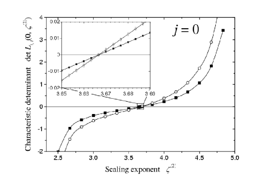
Figure 3: determinant and zero crossing for the sector $j=0$. The scaling exponent computed from the zero crossing is $\zeta^{(2)}_{0}\approx 0.667$.

For the higher $j$-sectors the agreement between the exponential and Gaussian models is not as perfect, indicating that the procedure is not exact. In Fig. 4 we present the determinant and zero crossings for $j=2$.

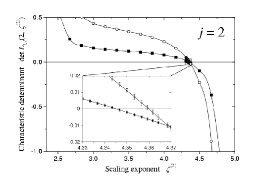
Figure 4: determinant and zero crossing for the sector $j=2$. The scaling exponent computed from the zero crossing is $\zeta^{(2)}_{2}\approx 1.36-1.37$.

From the inset we can read the exponents $\tilde{\zeta}_{2}^{(2)}=4.351$ and 4.366 for the exponential and Gaussian models respectively. This is in correspondence with $\zeta_{2}^{(2)}=1.351$ and $1.366$ respectively. These numbers are in excellent correspondence with the experimental measurements reported in [29, 13], cf. the next Section. The results for $j=4$ are presented in Fig. 5. Here the zero crossing, as seen in the inset, yields very close results for $\tilde{\zeta}_{4}^{(2)}$ between the exponential and Gaussian decay models, i.e. $\tilde{\zeta}_{4}^{(2)}\approx 4.99$. Note that this result is very close to the boundary of locality as discussed in [130]. Nevertheless the zero crossing is still easily resolved by the numerics, with the prediction that $\zeta_{4}^{(2)}\approx 1.99$. The simulation estimate of this number in [36] was $1.7\pm 0.1$. We note that while the result $\zeta_{4}^{(2)}\approx 1.99$ is not within the error bars of the simulational estimate, it is very possible that the closeness of the exponent to the boundary of the window of locality gives rise to very slow convergence to asymptotic scaling. We therefore have to reserve judgment about the agreement with simulations until larger scaling ranges were available.

Similar results are obtained for $j=6$, see Fig. 6. Also this case exhibits zero crossing close to the boundary of locality, with $\tilde{\zeta}_{6}^{(2)}\approx 6.98$. Again we find close correspondence between the exponential and Gaussian models. In terms of $\zeta^{(2)}$ this means $\zeta_{6}^{(2)}\approx 3.98$. This number appears higher than the simulational result from [36], which estimated $\zeta_{6}^{(2)}\approx 3.3\pm 0.3$. We note however that for $j=6$ the log-log plots measured in DNS [36] possess a short scaling range.

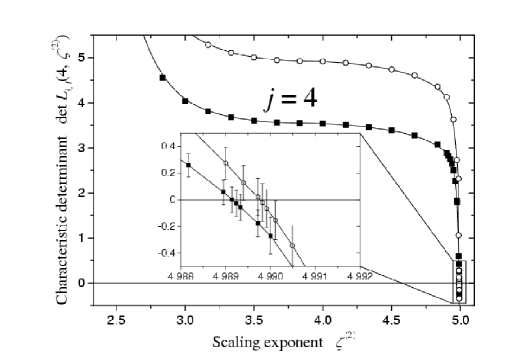
Figure 5: determinant and zero crossing for the sector $j=4$. The scaling exponent computed from the zero crossing is $\zeta^{(2)}_{4}\approx 1.99$.

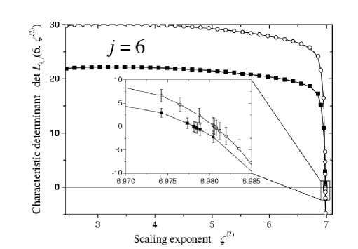
Figure 6: determinant and zero crossing for the sector $j=6$. The scaling exponent computed from the zero crossing is $\zeta^{(2)}_{6}\approx 3.98$.

Interestingly enough, the set of exponents $\zeta_{j}^{(2)}$=2/3, 1.36, 1.99 and 3.98 for $j=$0, 2, 4 and 6 respectively are in close agreement with the numbers obtained for the linear pressure model, $\xi_{j}^{(2)}$=2/3, 1.25226, 2.01922, 4.04843, for $j=0,2,4$ and 6 respectively. We reiterate at this point that the latter set is exact for the linear pressure model, whereas the former set is obtained within the closure approximation. In fact, the close correspondence is not so surprising since he linearization of Navier-Stokes equations for small anisotropy results in a linear operator which is very close to the one that exists naturally in the Linear Pressure Model. Numerical results [36, 15, 131] obtained at moderate Re and with strong anisotropies show a small disagreement with the numbers calculated in the closure approximation. We do not expect a much more precise theoretical evaluation of these exponents before numerical and experimental data at higher Re are obtained and the intermittency problem in the isotropic sector is fully settled.

6 Analysis of Experimental Data

The major difficulty in applying the SO(3) decomposition to experimental data lies in the fact that one never has the whole field $\mbox{\boldmath$u$}(\mbox{\boldmath$x$})$. We thus cannot project the statistical objects onto chosen basis functions $\mbox{\boldmath$B$}_{qjm}$ and simply integrate out all other contributions. Rather, we need to extract the wanted information laboriously by fitting partially resolved data, or to measure quantities that do not have projections on the isotropic sector, to see right away the anisotropic contributions. We begin with the first approach.

6.1 Anisotropic Contribution to the Statistics of the Atmospheric Boundary Layer

The atmospheric boundary layer offers a natural laboratory of turbulence that is unique in offering extremely high Re number. Students of turbulence interested in the scaling properties that are expected to be universal in the limit $Re\to\infty$ are thus attracted to atmospheric measurements. On the other hand the boundary layer suffers from strong inhomogeneity (explicit dependence of the mean velocity on the height) which leads to strong anisotropies such that the vertical and the horizontal directions are quite distinguishable. In addition, one may expect the boundary layer to exhibit large-scale quasi 2-dimensional eddys whose typical decay times and statistics may differ significantly from the generic 3-dimensional case. The aim of this section is to review systematic methods of data analysis that attempt to resolve such difficulties, leading to a useful extraction of the universal, 3-dimensional aspects of turbulence.

Obviously, to isolate tensorial components belonging to other than isotropic sectors one needs to collect data from more than one vector component of the velocity field. Having two probes is actually sufficient to read surprisingly rich information about anisotropic turbulence. In the experiments discussed in this subsection two types of geometry were employed, one consisting of two probes at the same height above the ground and the other with the two probes separated vertically. In both cases the inter-probe separation is orthogonal to the mean wind.

6.1.1 Experiments, Data Sets and the Extraction of Structure Functions

The results presented in this subsection are based on two experimental setups [29, 10, 13], which are denoted throughout as I and II respectively. In both setups the data were acquired over the salt flats in Utah with a long fetch. In set I the data were acquired simultaneously from two single hot wire probes at a height of 6 m above the ground, with a horizontal separation of 55 cm, nominally orthogonal to the mean wind. The Taylor microscale Reynolds number was about 10,000. Set II was acquired from an array of three cross-wires, arranged above each other at heights 11 cm, 27 cm and 54 cm respectively. The Taylor microscale Reynolds numbers in this set were 900, 1400 and 2100 respectively. Table 1 lists a few relevant facts about the data records analyzed here. The various symbols have the following meanings: $\overline{U}$ = local mean velocity, $u^{\prime}$ = root-mean-square velocity, $\bar{\epsilon}$ = energy dissipation rate obtained by the assumption of local isotropy and Taylor’s hypothesis, $\eta$ and $\lambda$ are the Kolmogorov and Taylor length scales, respectively, the microscale Reynolds number $R_{\lambda}\equiv u^{\prime}\lambda/\nu$, and $f_{s}$ is the sampling frequency.

For set I it is important to test whether the separation between the two probes is indeed orthogonal to the mean wind. (We do not need to worry about this point in set II, since the probes are above each other). To do so one computes the cross-correlation function $\langle u_{1}(t+\tau)u_{2}(t)\rangle$. Here, $u_{1}$ and $u_{2}$ refer to velocity fluctuations in the direction of the mean wind, for probes 1 and 2 respectively. If the separation were precisely orthogonal to the mean wind, this quantity should be maximum for $\tau=0$. Instead, for set I, it was found that the maximum shifted slightly to $\tau=0.022$ s, implying that the separation was not precisely orthogonal to the mean wind. To correct for this effect, the data from the second probe were time-shifted by 0.022 s. This amounts to a change in the actual value of the orthogonal distance. The effective distance is $\Delta\approx 54$ cm (instead of the 55 cm that was set physically).

Height	$\overline{U}$	$u^{\prime}$	$10^{2}\langle\bar{\epsilon}\rangle$,	$\eta$	$\lambda$	$R_{\lambda}$	$f_{s},$ per	# of
meters	ms-1	ms -1	m 2 s-3	mm	cm		channel, Hz	samples
6	4.1	1.08	$1.1$	0.75	15	10,500	10,000	$4\times 10^{7}$
0.11	2.7	0.47	$6.6$	0.47	2.8	900	5,000	$8\times 10^{6}$
0.27	3.1	0.48	2.8	0.6	4.4	1400	5,000	$8\times 10^{6}$
0.54	3.51	0.5	1.5	0.7	6.2	2100	5,000	$8\times 10^{6}$

Table 1: Data sets I (first line) and II (second-fourth lines).

The coordinates were chosen such that the mean wind direction is along the 3-axis, the vertical is along the 1-axis and the third direction orthogonal to these is the 2-axis. We denote these directions by the three unit vectors $\hat{\mbox{\boldmath$n$}}$, $\hat{\mbox{\boldmath$m$}}$, and $\hat{\mbox{\boldmath$p$}}$ respectively. The raw data available from set I is $u^{(3)}(t)$ measured at the positions of the two probes. In set II each probe reads a linear combination of $u^{(3)}(t)$ and $u^{(1)}(t)$ from which each component is extractable. From this raw data we would like to compute the scale-dependent structure functions, using the Taylor hypothesis to surrogate space for time. This needs a careful discussion.

6.1.2 Theoretical constructs: the Taylor Hypothesis, Inner and Outer Scales

Decades of research on the statistical aspects of thermodynamic turbulence are based on the Taylor Hypothesis [101], which asserts that the fluctuating velocity field measured by a given probe as a function of time, $\mbox{\boldmath$u$}(t)$ is the same as the velocity $\mbox{\boldmath$u$}(r/\overline{U})$ where $\overline{U}$ is the mean velocity and $r$ is the distance to a position “upstream” where the velocity is measured at $t=0$. The natural limitation on the Taylor hypothesis is provided by the typical decay time of fluctuations of scale $r$. Within a K41 scaling theory this time scale is the turn-over time $r/\sqrt{S(r)}$ where $S(r)\equiv S^{\alpha\alpha}(r)$. With this estimate the Taylor Hypothesis is expected to be valid when $\sqrt{S(r)}/\overline{U}\to 0$. Since $S(r)\to 0$ when $r\to 0$, the Taylor hypothesis becomes exact in this limit. We will use this to calibrate the units when we employ two different probes and read a distance from a combination of space and time intervals.

The Taylor hypothesis has also been employed when the mean velocity vanishes, and instead of $\overline{U}$ one uses the root-mean-square $u^{\prime}$. Ref.[132] has presented a detailed analysis of the consequences of the Taylor hypothesis on the basis of an exactly soluble model. In particular ways were proposed there to minimize the systematic errors introduced by the use of the Taylor hypothesis. In light of that analysis we will use here an “effective” wind $U_{eff}$ which for surrogating the time data of a single probe is made of a combination of the mean wind $\overline{U}$ and the root-mean-square $u^{\prime}$,

$$U_{eff}\equiv\sqrt{\overline{U}^{2}+(\tilde{b}u^{\prime})^{2}}\ ,$$ (171)

where $\tilde{b}$ is a dimensionless parameter. Evidently, when we employ the Taylor hypothesis in log-log plots of structure functions using time series measured in a single probe, the value of the parameter $\tilde{b}$ is irrelevant, changing just the (arbitrary) units of length (i.e the arbitrary intercept). When we used data collected from two probes, we mix read distance and surrogated distance, and the parameter $\tilde{b}$ becomes a unit fixer. The numerical value of this parameter is found in [132] by the requirement that the surrogated and directly measured structure functions coincide in the limit $r\to 0$. When we do not have the necessary data we will use values of $\tilde{b}$ suggested by the exactly soluble model treated in [132]. The choice of these values can be justified a posteriori by the quality of the fit of to the predicted scaling functions.

When we have two probes placed at different heights the mean velocity and $u^{\prime}$ as measured by each probe do not coincide. In applying the Taylor hypothesis one needs to decide which value of $U_{eff}$ is most appropriate. This question has been addressed in detail in ref.[132] with the final conclusion that the choice depends on the velocity profile between the probe. In the case of linear shear the answer is the precise average between the two probes,

$$U_{eff}\equiv\sqrt{{\overline{U_{1}}^{2}+\overline{U_{2}}\over 2}^{2}+\tilde{b}{{u_{1}^{\prime}}^{2}+{u_{1}^{\prime}}^{2}\over 2}}\ ,$$ (172)

where the subscripts 1,2 refer to the two probes respectively. In all the subsequent expressions we will therefore denote separations by $r$, and invariably this will mean Taylor-surrogated time differences. The effective velocity will be (171) or (172) depending on having probes at the same height or at different heights. The value of $\tilde{b}$ will be $\tilde{b}=3$ following ref.[132]. It can be shown that the computed scaling exponents are not sensitive to the changing $b$. (They change by a couple of percents upon changing $b$ by 30%.) In seeking scaling behavior one needs to find the inner and outer scales. Below the inner scale all structure functions have an analytic dependence on the separation, $S(r)\sim r^{2}$, and above the outer scale the structure functions should tend to a constant value. We look at the longitudinal structure functions

$$S^{33}(r)=\langle(u^{3}(x+r)-u^{3}(x))^{2}\rangle$$

computed from a single probe in set I and from the probe at $0.54$m in set II , see Fig.7.

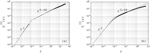
Figure 7: Raw log-log plot of the longitudinal component of the 2nd order structure function.

We simultaneously consider the transverse structure function

$$S^{11}(r)=\langle(u^{1}(x+r)-u^{1}(x))^{2}\rangle$$

computed from the probe at $0.54$m in set II, see Fig. 8.

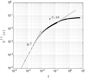
Figure 8: Raw log-log plot of the transverse component of the 2nd order structure function.

The spatial scales are computed using the local mean wind in both cases since the scaling exponent for the single-probe structure function are not expected to be affected by the choice of convection velocity. This choice does determine the value of $r$ corresponding to a particular time scale however. One may expect that any correction to the numerical value of $r$ is small for a different choice of convection velocity, and not crucial for the qualitative statements that follow. In Fig. 7 we clearly see the $r^{2}$ behavior characterizing the transition from the dissipative to the inertial range. As is usual, this behavior persists about a half-decade above the “nominal” Kolmogorov length scale $\eta$. There is a region of cross-over and then the isotropic scaling $\sim r^{0.68}$ expected for small scales in the inertial range begins. We thus have no difficulty at all in identifying the inner scale, it is simply revealed as a natural crossover length in this highly resolved data. We understand by now that we cannot expect to be able to fit with this single exponent for larger scales and must include scaling contributions due to anisotropy. We expect that the contributions due to anisotropy will account for scaling behavior up to the outer scale of a 3-dimensional flow patterns. The question therefore is how to identify what this large scale is. One approach would be to simply use the scale where the structure function tends to a constant, which corresponds to the scale across which the velocity signal has decorrelated. It becomes immediately apparent that this is not a reasonable estimate of the relevant large scale. Fig. 7 shows that the structure function stays correlated up to scales that are at least an order of magnitude larger than the height at which the measurement is made. On the other hand, if we look at the transverse structure function computed from the probe at $0.54$m, Fig. 8 we see that it ceases to exhibit scaling behavior at a scale that is of the order of the height of the probe. It appears that we are observing extremely flat eddys that are correlated over very long distances in the horizontal direction but have a comparatively small correlation lengths in the direction perpendicular to the boundary. Since we know that the presence of the boundary must limit the size of the largest 3-dimensional structures, the height of the probe should be something of an upper bound on the largest 3-dimensional flow patterns that we can detect in experiments. Thus we arrive at a qualitative understanding of the kind of flow that is observed in these atmospheric measurements. The size of the largest 3-dimensional structures is determined by the decorrelation length of the transverse structure function. This is because the transverse components of the velocity are unaffected by the extended, persistent, 2-dimensional eddys that govern the behavior of the longitudinal components. The theory of scaling behavior in 3-dimensional turbulence can usefully be applied to only those flow patterns that are truly 3-dimensional. The extended flat eddys must be described in terms of a separate theory, including maybe notions of 2-dimensional turbulence which has very different scaling properties [133]. Such considerations are outside the scope of this review. Rather, in the following analysis, the outer-scale was chosen to be of the order of the decorrelation length of the transverse structure function (where available) or of the height of the probe. We will see below that up to a factor of 2 these are the same; taking $L$ to be as twice the height of the probe is consistent with all data. We use this estimate in the study of both transverse and longitudinal objects.

6.1.3 Extracting the universal exponents of higher $j$ sectors

We consider the second order structure function

$$S^{\alpha\beta}({\bf r})=\langle(u^{\alpha}({\bf x}+{\bf r})-u^{\alpha}({\bf x}))(u^{\beta}({\bf x}+{\bf r})-u^{\beta}({\bf x}))\rangle.$$ (173)

The lowest order anisotropic contribution to the symmetric (in indices), even parity (in ${\bf r}$ due to homogeneity), second-order structure function is the $j=2$ component of the SO(3) symmetry group. Ref. [29] presents a derivation of the $m=0$ axisymmetric (invariant under rotation about the 3-axis) part of the $j=2$ contribution to this structure function in homogeneous turbulence. The derivation of the full $j=2$ contribution to the symmetric, even parity structure function appears in Appendix C. Fig. 9 b shows the fit to the structure function computed from a single probe in set I

$$S^{33}(r,\theta=0)=\langle(u_{1}^{(3)}(x+r)-u_{1}^{(3)}(x))^{2}\rangle,$$ (174)

where the subscript $1$ denotes one of the two probes, with just the $j=0$ contribution. The best-fit exponent for the range $0<r/\Delta<4.5$ is $\zeta^{(2)}_{0}=0.68\pm 0.01$ (Fig. 9 a). Above this range, was impossible to obtain a good fit to the data with just the isotropic exponent and Fig. 9 b shows the peel-off from isotropic behavior above $r/\Delta=4$.

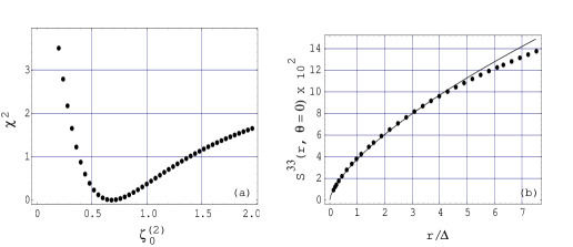
Figure 9: The single-probe structure function computed from data set I. (a) shows the $\chi^{2}$ minimization by the best-fit value of the exponent in the isotropic sector $\zeta_{0}^{(2)}\approx 0.68$ for the single-probe structure function in the range $0<r/\Delta<4.5$. (b) shows the fit using the best value of $\zeta_{0}^{(2)}$ obtained in (a), indicating the peel-off from isotropic behavior at the end of the fitted range.

To find the $j=2$ anisotropic exponent one needs to use data taken from the two probes. To clarify the procedure we show in Fig.10 the geometry of set I.

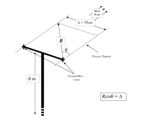
Figure 10: Diagrammatic illustration of the experimental set-up. Shown is the positioning of the probes with respect to the mean wind and how the Taylor hypothesis is employed

What was computed is actually

$$S^{33}(r,\theta)=\langle[u^{(3)}_{1}(U_{eff}t+U_{eff}t_{\tilde{r}})-u^{(3)}_{2}(U_{eff}t)]^{2}\rangle$$

Here $\theta=\arctan(\Delta/U_{eff}t_{\tilde{r}})$, $t_{\tilde{r}}=\tilde{r}/U_{eff}$, and $r=\sqrt{\Delta^{2}+(\bar{U}_{eff}t_{\tilde{r}})^{2}}$. $U_{eff}$ was as in Eq.(171) with $b=3$. We will refer from now on to such quantities as

$$S^{33}(r,\theta)=\langle(u_{1}^{(3)}(x+r)-u_{2}^{(3)}(x))^{2}\rangle\ .$$ (175)

Next, one may fix the scaling exponent of the isotropic sector as $0.68$ and find the $j=2$ anisotropic exponent that results from fitting to the full $j=2$ tensor contribution. Finally, one needs to fit the objects in Eqs. (174) and (175) to the sum of the $j=0$ (with scaling exponent $\zeta^{(2)}_{0}=0.68$) and the $j=2$ contributions (see Appendix C)

$$S^{33}(r,\theta)=S^{33}_{j=0}(r,\theta)+S^{33}_{j=2}(r,\theta)=c_{0}\left({r\over\Delta}\right)^{\zeta^{(2)}_{0}}\Big{[}2+\zeta^{(2)}_{0}-\zeta^{(2)}_{0}\cos^{2}\theta\Big{]}$$ (176)

$$+ a\left({r\over\Delta}\right)^{\zeta_{2}^{(2)}}\Big{[}(\zeta_{2}^{(2)}+2)^{2}-\zeta_{2}^{(2)}(3\zeta_{2}^{(2)}+2)\cos^{2}\theta+2\zeta_{2}^{(2)}(\zeta_{2}^{(2)}-2)\cos^{4}\theta\mbox{\boldmath$i$}g]$$

$$+ b\left({r\over\Delta}\right)^{\zeta_{2}^{(2)}}\Big{[}(\zeta_{2}^{(2)}+2)(\zeta_{2}^{(2)}+3)-\zeta_{2}^{(2)}(3\zeta_{2}^{(2)}+4)\cos^{2}\theta+(2\zeta_{2}^{(2)}+1)(\zeta_{2}^{(2)}-2)\cos^{4}\theta\Big{]}$$

$$+ a_{9,2,1}\left({r\over\Delta}\right)^{\zeta_{2}^{(2)}}\Big{[}-2\zeta_{2}^{(2)}(\zeta_{2}^{(2)}+2)\sin\theta\cos\theta+2\zeta_{2}^{(2)}(\zeta_{2}^{(2)}-2)\cos^{3}\theta\sin\theta\Big{]}$$

$$+ a_{9,2,2}\left({r\over\Delta}\right)^{\zeta_{2}^{(2)}}\Big{[}-2\zeta_{2}^{(2)}(\zeta_{2}^{(2)}-2)\cos^{2}\theta\sin^{2}\theta\Big{]}$$

$$+ a_{1,2,2}\left({r\over\Delta}\right)^{\zeta_{2}^{(2)}}\Big{[}-2\zeta_{2}^{(2)}(\zeta_{2}^{(2)}-2)\sin^{2}\theta\Big{]}.$$

The above fit was performed using values of $\zeta_{2}^{(2)}$ ranging from $0.5$ to $3$. The best value of this exponent is the one that minimizes the $\chi^{2}$ for the fits. From Fig.11 one may read the best value to to be $1.38\pm 0.15$. The fits with this choice of exponent are displayed in Fig.12. The corresponding values of the 5 fitted coefficients can be found in the paper [29]. The range of scales that are fitted to this expression is $1<r/\Delta<25$. We thus conclude that that structure functions which is symmetric in $r$ exhibits scaling behavior over the whole scaling range, but this important fact is missed if one does not consider a superposition of the $j=0$ and $j=2$ contributions.

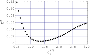
Figure 11: The $\chi^{2}$ minimization by the best-fit value of the exponent in the $j=2$ anisotropic sector from the fit to both the $\theta=0$ and the $\theta$-dependent structure function in the range $0<r/\Delta<25$.

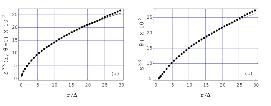
Figure 12: The structure functions computed from data set I and fit with the $j=0$ and full $j=2$ tensor contributions using the best fit values of exponents $\zeta^{(2)}_{0}=0.68$ and $\zeta_{2}^{(2)}=1.38$ in the range $0<r/\Delta<25$. Panel (a) shows the fit to the single-probe ($\theta=0$) structure function and panel (b) shows the fit to the $\theta$-dependent structure function.

Finally, let us note that the value of the exponent is perfectly in agreement with the analysis of numerical simulations [34] in which one can comfortably integrate the structure function against the basis functions, eliminating all contributions except $j=2$ (see next section).

6.1.4 Extracting the j=1 component

In homogeneous flows, it follows from symmetry and parity that the often computed and widely analyzed structure function as defined in Eq. (173) does not possess any contribution from the $j=1$ sector. The lowest order anisotropic contribution belongs to the $j=2$ sector. In order to isolate the scaling behavior of the $j=1$ contribution in atmospheric shear flows we must either explicitly construct a new tensor object which will allow for such a contribution, or see if it can be extracted from the structure function itself computed in the case of inhomogeneity. We have pursued both avenues. In the former, we construct the tensor

$$T^{\alpha\beta}({\mbox{\boldmath$r$}})=\langle u^{\alpha}({\mbox{\boldmath$x$}}+{\mbox{\boldmath$r$}})-u^{\alpha}({\mbox{\boldmath$x$}}))(u^{\beta}({\mbox{\boldmath$x$}}+{\mbox{\boldmath$r$}})+u^{\beta}({\mbox{\boldmath$x$}}))\rangle.$$ (177)

It is easily seen that the function vanishes both in the case of $\alpha=\beta$ and when $r$ is in the direction of homogeneity. From data set II we can calculate this function for non-homogeneous (in the shear direction) scale-separations. In general, this will exhibit mixed parity and symmetry and therefore, to minimize as far as possible the final number of fitting parameters we look at only the antisymmetric contribution. We derive the tensor contributions in the $j=1$ sector for the antisymmetric case in Appendix D and use this to fit for the unknown $j=1$ exponent. Below we describe the results of this analysis. Next, we computed the $\theta$-dependent structure function from set II. We expect that this could exhibit the $j=1$ component as inhomogeneity does not allow us to apply incompressibility in the different symmetry and parity sectors to eliminate this contribution as in the case of the homogeneous structure function. This structure function is symmetric but of mixed parity. We derive the tensor contributions in the $j=1$ sector for the symmetric case in Appendix D and use this to fit for the $j=1$ exponent.

6.1.5 Antisymmetric Contribution

We consider the tensor object in Eq. (177). In order to have as few parameters as possible in the fitting procedure, we take the antisymmetric part

$${\widetilde{T}}^{\alpha\beta}({\mbox{\boldmath$r$}})={T^{\alpha\beta}({\mbox{\boldmath$r$}})-T^{\beta\alpha}({\mbox{\boldmath$r$}})\over 2}=\langle u^{\alpha}({\mbox{\boldmath$x$}})u^{\beta}({\mbox{\boldmath$x$}}+{\mbox{\boldmath$r$}})\rangle-\langle u^{\beta}({\mbox{\boldmath$x$}})u^{\alpha}({\mbox{\boldmath$x$}}+{\mbox{\boldmath$r$}})\rangle$$

which will only have contributions from the antisymmetric $j=1$ basis tensors. An additional useful property of this object is that it does not have any contribution from the isotropic helicity-free $j=0$ sector due to its antisymmetry. This allows us to isolate the $j=1$ contribution and determine its scaling exponent $\zeta_{1}^{(2)}$ starting from the smallest scales available. Using data from the probes at $0.27$m (probe 1) and at $0.11$m (probe 2) we calculate

$${\widetilde{T}}^{31}({\mbox{\boldmath$r$}})=\langle u_{2}^{(3)}(\mbox{\boldmath$x$})u_{1}^{(1)}(\mbox{\boldmath$x$}+\mbox{\boldmath$r$})\rangle-\langle u_{1}^{(3)}(\mbox{\boldmath$x$}+\mbox{\boldmath$r$})u_{2}^{(1)}(\mbox{\boldmath$x$})\rangle\ ,$$

where again super-scripts denote the velocity component and sub-scripts denote the probe at which this component is measured. We want to fit this object to the tensor form derived in Appendix (D), namely:

$${\widetilde{T}}^{31}(r,\theta,\phi=0)=-a_{3,1,0}r^{\zeta_{1}^{(2)}}\sin\theta+a_{2,1,1}r^{\zeta_{1}^{(2)}}+a_{3,1,-1}r^{\zeta_{1}^{(2)}}\cos\theta.$$

Fig. 13 gives the $\chi^{2}$ minimization of the fit as a function of $\zeta_{1}^{(2)}$ and we use the best value of $1\pm 0.15$ for the final fit. This is shown in the left panel.

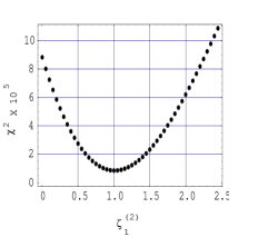
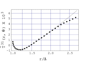
Figure 13: Right: the $\chi^{2}$ minimization by the best-fit value of the exponent $\zeta_{1}^{(2)}$ of the $j=1$ anisotropic sector from the fit to $\theta$-dependent ${\widetilde{T}}^{31}(r,\theta)$ function in the range $0<r/\Delta<2.2$. Left: The fitted ${\widetilde{T}}^{31}(r,\theta)$ function. The dots indicate the data and the line is the fit.

The fit in Fig. 13 peels off at the end of the fitted range. The maximum range over which one can fit is of the order of the height of the probes and again, this is consistent with the considerations presented above.

6.1.6 Symmetric Contribution

Finally, we compute the structure function Eq. (175) where the subscripts denote probe 1 at $0.27$m and probe 2 at $0.11$cm. As discussed in Appendix (D), since the scale separation has an inhomogeneous component, we expect a contribution from the $j=1$ anisotropic sector and we would like to extract what the scaling exponent in this sector is. Note that the $j=0$ sector contributes two independent tensor forms with coefficients we will denote by $c_{1}$ and $c_{2}$, since incompressibility does not provide a constraint to relate them. This fact combined with Eq. (222) gives us the the tensor form to which we must fit our function

$$S^{33}(r,\theta)=c_{1}r^{\zeta_{0}^{(2)}}+c_{2}r^{\zeta_{0}^{(2)}}\cos^{2}\theta+a_{1,1,0}r^{\zeta_{1}^{(2)}}\cos\theta+a_{7,1,0}r^{\zeta_{1}^{(2)}}2\cos\theta$$ (178)

$$+a_{9,1,0}r^{\zeta_{1}^{(2)}}\cos^{3}\theta+a_{8,1,1}r^{\zeta_{1}^{(2)}}(-2\cos\theta\sin\theta)+a_{1,1,-1}r^{\zeta_{1}^{(2)}}\sin\theta+a_{9,1,-1}r^{\zeta_{1}^{(2)}}\cos^{2}\theta\sin\theta$$

We fix the exponent $\zeta^{(2)}_{0}$ to be $0.68$ and perform fits with varying values of $\zeta_{1}^{(2)}$ for 8 unknown coefficients. The best value of $\zeta_{1}^{(2)}$ is obtained for the range $0<r/\Delta<4.2$ and is $1.05\pm 0.15$ as is shown in Fig. 14. In the left panel we show the fit to the data using this value of the exponent. -8.2 The fit peels off at the end of the fitted range at the scale on the order of twice the height of the probe, consistent with the earlier discussion. There does not exist a well-defined $\zeta_{1}^{(2)}$ as given by the standard $\chi^{2}$ minimization procedure for ranges smaller or larger than that fitted for in Fig. 14. The quality of the fit is good although, as was expected from the large number of parameters in the fitting function Eq. (178), $\chi^{2}$ as a function of the $\zeta_{1}^{(2)}$ is not as smooth as for all previous fits and its minimum is a relatively weak one. Therefore, we present this result mainly as it provides support to that of the antisymmetric case in the previous section.

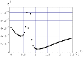
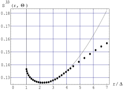
Figure 14: Right: the $\chi^{2}$ minimization by the best-fit value of the exponent $\zeta_{1}^{(2)}$ of the $j=1$ anisotropic sector from the fit to $\theta$-dependent inhomogeneous structure function in the range $0<r/\Delta<2.2$. Left: The fit to the inhomogeneous structure function computed as in Eq.(178). The dots indicate the data and the line is the fit.

dots

6.1.7 Summary and conclusions

In summary, we considered the 2nd order tensor structure functions of velocity differences in the atmospheric boundary layers. The following conclusions appear important:

1. The atmospheric boundary layer exhibits 3-dimensional statistical turbulence intermingles with activities whose statistics are quite different. The latter are eddys with quasi-two dimensional nature, correlated for hundreds of meters, having little to do with the three-dimensional fluctuations discussed above. We found that the

2. We found that the “outer scale of turbulence” as measured by the three-dimensional statistics is of the order of twice the height of the probe.

3. The inner scale is the the usual dissipative crossover, which is clearly seen as the scale connecting two different slopes in log-log plots.

4. Between the inner and the outer scales the sum of the components up to $j=2$ appears to offer an excellent representation of the structure function.

5. The scaling exponents $\zeta_{j}^{(2)}$ are measured as $0.68\pm 0.01,~{}1\pm 0.15,~{}1.38\pm 0.10$ for $j=0,1,2$ respectively.

We note that as far as the low order $j$ sectors are concerned, the picture that emerges for Navier-Stokes turbulence is not different from the linear advection problems that were treated in the previous section. If the trends seen here continue for higher $j$ values, we can rationalize the apparent tendency toward isotropy with decreasing scales. If indeed every anisotropic contribution introduced by the large scale forcing (or boundary conditions) decays as $(r/L)^{\zeta_{j}^{(2)}}$ with increasing $\zeta_{j}^{(2)}$ as a function of $j$, then obviously when $r/L\to 0$ only the isotropic contribution survives. This is a pleasing notion that justifies the modeling of turbulence as isotropic at the small scales.

6.2 Homogeneous Shear

In this subsection we discuss recent experiments in which anisotropy is created without inhomogeneity [7, 30, 31]; such experiments are particularly appealing for our purposes. Homogeneous-shear flow can be realized in a wind tunnel by using a variable solidity screen followed by flow straighteners. Such a set-up results in a shear flow that remains approximately constant for the length of the tunnel. To produce high Reynolds numbers one places an active grid before the shear generating screen [7]. In this way $Re_{\lambda}$ can be as high as 1000.
To assess directly the effects of anisotropy it is useful to measure statistical objects that vanish identically in the isotropic sector. A possible choice is the set of skewness and hyper-skewness [14, 38, 134] as explained in Sect. (2.5). Other purely anisotropic inertial range observables can be defined by mixing longitudinal and transversal increments with an odd number of transversal components:

$$S^{(p,2q+1)}(\mbox{\boldmath$r$})=\left<\delta u_{\ell}^{p}(\mbox{\boldmath$r$})\delta u_{t}^{2q+1}(\mbox{\boldmath$r$})\right>.$$ (179)

Systematic measurements of these anisotropic mixed correlation functions was reported in [30, 31, 10]. From the experimental data it is not possible to exactly disentangle different anisotropic projections in different sectors. This is because SO(3) projection requires the knowledge of the whole velocity field in a 3d sub-volume, something clearly out of reach in any experimental apparatus. The simplest working hypotheses one can make is that, due to the hierarchical organization of anisotropic scaling exponents, the statistical behavior of quantities as (179) is dominated, at scales small enough, by the leading $j=2$ sector. In other words, the experimental measurements of the scaling properties of (179) is the best estimate of the exponent $\zeta_{2}^{(n=p+2q+1)}$. In [30, 31] the plots of purely anisotropic quantities like (179) up to order $n=8$ with $n=p+2q+1$ were shown. The data clearly shows that these purely anisotropic structure functions have quite good power-laws behavior with exponents that are sub-leading with respect to the exponents of the isotropic structure functions of the same order, $n$. For example $S^{(1,3)}(r)\sim r^{1.56}$ while the fourth-order longitudinal structure function in isotropic ensembles is known to scale as $S^{(4,0)}(r)\sim r^{1.27}$. Similar qualitative and quantitative results were obtained by analyzing data from an atmospheric boundary layer in [10] and in the boundary layer close to a wall [33]. In the latter two works, a phenomenological fitting procedure to the large scale behavior allowed the authors to find a power law for the anisotropic structure functions which pertain to a much larger range of scales. We draw the reader’s attention to the discrepancy in the best fit for the scaling exponents founds for $S^{(1,3)}(r)$ and $S^{(3,1)}(r)$ in [30, 31]. Similar discrepancies are also reported for higher order structure functions. In our view, this cannot be taken as evidence that there is a $q$-dependence of the scaling exponents of the SO(3) projections. First, the anisotropic exponents are relatively inaccurate due to statistical errors; the amplitudes of the anisotropic fluctuations are relatively small. Second, as already said, the experimental data cannot disentangle exactly the contribution of the $j=2$ sector. Therefore, it may well be that contributions from the $j=4$ (and higher) sectors affect differently the correlation functions with different tensorial structure. Similarly, other experimental investigation focused on the SO(3) decomposition [135, 136, 32] have found results depending on the geometric set-up of the analyzing probes. The experimental analysis of anisotropic turbulence via the SO(3) decomposition is at its infancy; more refined experimental techniques are needed before a firm conclusion can be reached on these issues.

6.2.1 Explanation of Persistence of Anisotropies

As discussed in Sect. (2.5) there are numerical and experimental evidences of the persistence of small-scale anisotropic fluctuations in various instances [55, 7, 10, 21, 35]. The issue has many important consequences. We would like to refer to the violation of the return-to-isotropy in different meanings [35]. A strong violation would be implied if the following set of inequalities between different anisotropic exponents of the same correlation function were broken:

$$\zeta^{(n)}_{0}<\zeta^{(n)}_{1}<\cdots<\zeta^{(n)}_{j}\ ,$$ (180)

i.e. if one, or more, anisotropic sector becomes leading with respect to the isotropic one. This would destroy the phenomenology of turbulence as developed since Kolmogorov’s theory in 1941. Turbulence would become more and more anisotropic at smaller and smaller scales. As a result, strong non-universalities in small-scales statistics would show up depending on which anisotropic sector is switched on/off by the large-scale forcing. A strong violation of the return-to-isotropy postulate has never been observed in Navier-Stokes turbulence. On the other hand, when the hierarchy (180) holds, any dimensionless anisotropic observables made of ratios between anisotropic and isotropic projections of the same correlation function vanishes in the small-scales limit. For example, focusing on the decomposition of longitudinal structure functions (44) we may write:

$$\lim_{r\rightarrow 0}\frac{S_{jm}^{(n)}(r)}{(S_{00}^{(n)}(r))}\;\sim r^{\zeta^{(n)}_{j}-\zeta^{(n)}_{0}}\rightarrow 0.$$ (181)

A new phenomenon occurs when anisotropic fluctuations are assessed by using dimensionless observables made of different correlation functions. For instance, by using again the SO($3$) decomposition of longitudinal structure function (44) one may build up anisotropic observables defined as:

$$R_{jm}^{(n)}(r)=\frac{S_{jm}^{(n)}(r)}{(S_{00}^{(2)}(r))^{n/2}}\;\sim r^{\chi_{j}^{(n)}}\;\;\;\mbox{ with }\;\;{\chi_{j}^{(n)}=\zeta_{j}^{(n)}-{n\over 2}\zeta_{0}^{(2)}}\ .$$ (182)

This is the $n$th order moment of the velocity probability density function, normalized by its isotropic second order moments. The quantities defined in (182) must be exactly zero in isotopic ensembles, and should go to zero as power laws, $R_{jm}^{(n)}(r)\sim r^{j/3}$, in an anisotropic ensemble in which the dimensional scaling (46) is satisfied. On the other hand, results from experiments and numerics show a much slower decay, and, in some cases, no decay at all [7, 35]. We refer to this phenomenon as weak violation of the return-to-isotropy. Such a weak violation is not in contradiction with the inequalities (180); there the relative importance of anisotropic fluctuations with respect to isotropic fluctuation of the same correlation function are implied. The violation of the dimensional recovery-of-isotropy is simply due to the existence of anomalous scaling in the anisotropic sectors. Indeed, in this case, the exponents, $\chi_{j}^{(n)}$, governing the LHS of (182) can assume values much smaller than the dimensional estimate (including negative values!). This is exactly what is observed in the experiments and numerics. From Table 3 one realizes that due to the presence of anomalous scaling in the anisotropic sectors we have a slow recovery-of-isotropy, in agreement with what was explained before.

The anisotropic observables built in terms of the generalized flatness or skewness discussed in section (2.5) are nothing but Eq. (182) evaluated at the dissipative length scale, $r=\eta$. Therefore, the “persistence-of-anisotropies” discussed in [21, 7] can be explained invoking the very same reasoning.

6.2.2 Summary of experimental results: universality of the anisotropic sectors

Comparing the results obtained in [30, 31, 10] the following picture emerges. First, all the correlation functions up to $n=10$, show anomalous scaling behavior, where anomalous is meant with respect to the dimensional Lumley-like prediction discussed in Sect. (4.4). Second, the values of scaling exponents extracted from the two different experiments [31] and [10] are in good qualitative agreement (see Table 2).

$(p,2q+1)$	(1,1)	(1,3)	(3,1)	(5,1)	(3,3)	(1,5)	(7,1)	(5,3)	(3,5)
WS	1.05	1.56	1.42	2.02	1.89	1.71	2.33	2.22	1.99
KS	1.22,1.12	1.58,1.54	-	-	2.14,2.00	-	-	-	-

Table 2: Measured scaling exponents for $S^{(p,2q+1)}(\mbox{\boldmath$r$})$ of various orders in two experiments. WS corresponds to [31] and KS to [10]

This is an important first confirmation of the universality of scaling exponents in the $j=2$ anisotropic sector. Finally, there exists a clear hierarchy between isotropic and anisotropic scaling exponents, the latter being always larger for any given order, $n$ of the correlation function. This hierarchical organization is the necessary and sufficient requirement for the return-to-isotropy to hold, i.e. the small scales statistics of any correlation function is dominated by the isotropic fluctuations. Nevertheless the gap between isotropic and anisotropic exponents, $\zeta_{0}^{(n)}-\zeta_{2}^{(n)}$, tends to shrink when $n$ increases, implying that anisotropic contributions may exhibit important sub-leading effects also at very high Re.

7 Analysis of DNS Data

Direct numerical simulations of turbulence are natural grounds where the utility of the SO($3$) decomposition can be exploited to its maximum benefit. The reason for this is that numerical simulations, in contrast to current experiments, provide access to the full velocity field at all points of the turbulent domain. Therefore, the full SO($3$) decomposition can be realized, without the constraints of best-fits to partial data. Given a tensor structure function $\mbox{\boldmath$S$}^{(n)}(\mbox{\boldmath$r$})$, cf. Eq.(31), we can integrate it against the spherical tensors, $\mbox{\boldmath$B$}^{(n)}_{qjm}(\hat{\mbox{\boldmath$r$}})$ [e.g., (35)], on a sphere of radius $r$. These integrations yield the projection of the structure function on the different sectors of the SO($3$) group, by virtue of the orthogonality of the basis tensors. On the other hand DNS suffer from limited Reynolds numbers; consequently they have relatively short inertial ranges.

Prior to the introduction of the SO(3) decomposition the numerical investigations of anisotropic flows were focused on either single point or two-points correlations, limited, often, to the analysis of the Fourier transforms in wavevector space. The most recent, highly-resolved, numerical investigation of this kind was reported in [37]; there the full tensorial properties of the Fourier transform of the two-point velocity correlation, $Q^{\alpha\beta}(\mbox{\boldmath$k$})\stackrel{{\scriptstyle\mathrm{def}}}{{=}}\int d\mbox{\boldmath$r$}e^{i\mbox{\boldmath$k$}\mbox{\boldmath$r$}}\langle u^{\alpha}(\mbox{\boldmath$x$}+\mbox{\boldmath$r$})u^{\beta}(\mbox{\boldmath$x$})\rangle$, were calculated in a homogeneous shear [6, 137]. The main result is a confirmation of Lumley’s prediction for the scaling exponent of the purely anisotropic co-spectrum:

$$E^{\alpha\beta}(k)\sim k^{-7/3}\;\;\;\mbox{where}\;\;\;E^{\alpha\beta}(k)=\int_{{k\over 2}<|\mbox{\boldmath$p$}|<2k}d\mbox{\boldmath$p$}Q^{\alpha\beta}(\mbox{\boldmath$p$})\ ,$$ (183)

where $\alpha\neq\beta$ to eliminate the isotropic contribution. Only recently DNS were performed to probe the anisotropic component in a systematic way by exploiting the SO($3$) decomposition [34, 36, 138, 15, 131]. Here we review the main findings, showing that

1. The scaling laws (log-log plots) at moderate Reynolds numbers are significantly improved by projecting the raw correlation functions onto each $j$-sectors. The improvement is particular noticeable whenever strong anisotropies are present in the system, as in the case of channel flows [34, 138];

2. Anisotropic sectors with $j\geq 2$ (inaccessible in present experimental data) possess good scaling laws [36, 15];

3. The scaling exponents are discrete and increasing as a function of $j$.

4. The exponents are anomalous; i.e. they differ from the dimensional prediction (46).

5. There exists preliminary evidence that also for $j>2$, the anomalous exponents are universal, i.e. the scaling properties are independent of the external forcing mechanism [131].

DNS were performed both in wall-bounded flows and in homogeneous (but anisotropic) turbulence. In wall-bounded flows the anisotropies are accompanied by inhomogeneous effects. The presence of such effects may spoil the very meaning of scaling, and the SO($3$) decomposition should be supplemented by some tool to project on the homogeneous components. Otherwise, the SO(3) decomposition must be used carefully, and locally, only in those regions of the tested flow where inhomogeneous effects are confined mostly to large-scales [34, 138]. In the second part of this section, we discuss numerical experiments built such as to have a perfectly homogeneous and anisotropic statistics at all scales. One such example is homogeneous shear flows [38, 17]. More recently, other homogeneous anisotropic flows have been invented and simulated, in particular the random-Kolmogorov-flow [36, 15, 139] and a convective cell with an imposed linear mean profile of temperature [131].

7.1 Anisotropic and inhomogeneous statistics: Channel flows

In this section, we discuss the analysis of a DNS of a channel flow using the SO($3$) decomposition. The coordinates are chosen such that $\hat{x}$, $\hat{y}$ and $\hat{z}$ are the stream-wise, span-wise, and wall-normal direction respectively. The simulation was done on a grid with $256$ points in the stream-wise direction and $128\times 128$ points in the two other directions. The boundary conditions were periodic in the span-wise and stream-wise directions and no-slip on the walls. The Reynolds-number based on the Taylor micro-scale was quite moderate, $R_{\lambda}\approx 70$ at the center of the channel $(z=64)$. The simulation was fully symmetric with respect to the central plane. For more details on the averaged quantities and on the numerical code, see refs. [34, 140, 141].

The analysis focused on longitudinal second-, forth- and sixth-order structure functions:

$$S^{(n)}(\mbox{\boldmath$r$}^{c},\mbox{\boldmath$r$})\equiv\left<\big{[}\delta u_{\ell}(\mbox{\boldmath$r$}^{c},\mbox{\boldmath$r$})\big{]}^{n}\right>,\quad\delta u_{\ell}(\mbox{\boldmath$r$}^{c},\mbox{\boldmath$r$})\equiv\hat{\mbox{\boldmath$r$}}\cdot\big{[}\mbox{\boldmath$u$}(\mbox{\boldmath$r$}^{c}+\mbox{\boldmath$r$},t)-\mbox{\boldmath$u$}(\mbox{\boldmath$r$}^{c}-\mbox{\boldmath$r$},t)\big{]}\ .$$

The $\mbox{\boldmath$r$}^{c}$ coordinate specifies the location of the measurement (i.e., the center of mass of the two measurement points), and $2\mbox{\boldmath$r$}$ is the separation vector. Previous analysis of the same data-base [140] as well as of other DNS [142] and experimental data [9, 72] in anisotropic flows found that the scaling exponents of energy spectra, energy co-spectra and of longitudinal structure functions exhibit strong dependence on the position $r_{c}$. For example, in [18] the authors studied the longitudinal structure functions at fixed distances from the walls:

$$S^{(n)}(r,z)\equiv\langle(u_{x}(x+r,y,z)-u_{x}(x,y,z))^{n}\rangle_{z}$$

where $\langle\cdots\rangle_{z}$ denotes a spatial average on a plane at a fixed height $z$, $1<z<64$. For this set of observables they found that: (i) These structure functions did not exhibit clear scaling behavior as a function of the distance $r$. Consequently, one needed to resort to Extended-Self-Similarity (ESS) [51] in order to extract a set of relative scaling exponents $\hat{\zeta}^{(n)}(z)\equiv\zeta^{(n)}(z)/\zeta^{(3)}(z)$; (ii) the relative exponents, $\hat{\zeta}^{(n)}(z)$ depended strongly on the height $z$. Moreover, only at the center of the channel and very close to the walls the error bars on the relative scaling exponents extracted by using ESS were small enough to claim the very existence of scaling behavior in any sense. Similarly, an experimental analysis of a turbulent flow behind a cylinder [72] showed a strong dependence of the relative scaling exponents on the position behind the cylinder for not too big distances from the obstacle, i.e. where anisotropic effects may still be relevant in a wide range of scales. In the following we present an interpretation of the variations in the scaling exponents observed in non-isotropic and non-homogeneous flows upon changing the position in which the analysis is performed. In particular, we will show that decomposing the statistical objects into their different $(j,m)$ sectors rationalizes the findings, i.e. scaling exponents in given $(j,m)$ sector appear quite independent of the spatial location; only the amplitudes of the SO(3) decomposition depend strongly on the spatial location. The analysis showed three major results. The first was the vast improvement in scaling behavior of the structure functions as a result of the decomposition. A typical example is found in Fig.(15 )

Figure 15: Log-log plot of the isotropic sector of the 4th order structure function $S^{(4)}_{0,0}(r)$, vs. $r$ at the center of the channel $r^{c}_{z}=64$ (+). The data represented by ($\times$) correspond to the raw longitudinal structure function, $S^{(4)}(r^{c}_{z}=64,r\hat{x})$ averaged over the central plane only. The dashed line corresponds to the intermittent isotropic high-Reynolds numbers exponents $\zeta^{(4)}_{0}=1.28$.

where the raw fourth-order structure function, evaluated on the central plane, is compared to its $j=0$ component. Without the SO($3$) decomposition there is no scaling behavior at all and one needs ESS to estimate the scaling exponents. On the other hand, the $j=0$ component of the structure function shows a clear scaling behavior with the expected exponent, $\zeta^{(4)}_{0}=1.28$. This strengthens the foliation hypothesis, according to which, the raw structure function is a superposition of power laws from different sectors of the SO($3$) group. Such a sum looses its scale invariance once the weights of the different exponents are of the same order and the inertial range is small. In such cases, one needs the SO($3$) decomposition to isolate the different sectors and retain scale invariance.

Figure 16: Logarithmic local slopes of the ESS plot of raw structure function,$\frac{dlog(S^{(4)}(r,r_{c})}{dlog(S^{(2)}(r,r_{c})}$, of order 4 versus raw structure function of order 2 at $r_{c}^{z}=64$ ($\times$), at $r_{c}^{z}=32$ ($\star$) and of the $j=0$ projection, $\frac{dlog(S^{(4)}_{00}(r,r_{c})}{dlog(S^{(2)}_{00}(r,r_{c})}$, centered at $r_{c}^{z}=64$ ($+$), and at $r_{c}^{z}=32$($\Box$). Also two horizontal lines corresponding to the high-Reynolds number limit, $1.82$, and to the K41 non-intermittent value, $2$, are shown.

A second prominent result is the apparent universality of the isotropic exponents. To show this in [34] the local slopes, $\frac{dlog(S^{(4)}_{00}(r)}{dlog(S^{(2)}_{00}(r)}$, of the ESS curves of the isotropic forth-order structure-function versus the isotropic second-order structure function were calculated at varying the distance from the wall. Despite their different locations, all curves show the same ESS slope 1.82, which is the expected (anomalous) value. In Fig.(16) one picture is presented for the logarithmic local slopes at two different distances from the channel boundary. To appreciate the improvements in scaling and universality, also the slopes of the ESS on the raw structure functions are presented Finally, the analysis provided another evidence that the $j=2$ scaling exponent of the second order structure function is about $4/3$, which is the dimensional theoretical prediction given in (27) (see also [8, 90, 92, 91, 15]). Considering the relatively low Reynolds-number and the fact that the prefactors $a_{j,m}$ in the SO($3$) decomposition (180) are non-universal, together with the experimental result reported in [29, 10, 30, 31], these findings give strong support to the view that the scaling exponent in the $j=2$ sector is universal. Before concluding this section we cite that SO(3) and SO(2) decomposition have also been exploited in the analysis of channel flow data to highlights the importance of structures as streaks and hairpin filaments typical of many wall bounded flow [138]. Preliminary investigation of the importance of SO(3) decomposition to evaluate the performance of sub grid models used in Large Eddy Simulations [143] have also been reported in [139].

7.2 Anisotropic-homogeneous flows

Direct numerical simulations offer the unique opportunity to study the physics of anisotropy in ideal situations, that is in perfectly homogeneous flows. Recently, considerable effort has been spent on simulating a Random-Kolmogorov-Flow (RKF) [36, 15, 139]. The RKF is fully periodic, incompressible and with anisotropic large-scale energy injection. A convenient choice for the forcing is ${\mbox{\boldmath$f$}}=(0,0,f_{z}(x))$ with $f_{z}(x)=F_{1}\cos[2\pi x/L_{x}+\phi_{1}(t)]+F_{2}\cos[4\pi x/L_{x}+\phi_{2}(t)]$, with constant amplitudes $F_{1,2}$ and independent, uniformly distributed, $\delta$-correlated in time and with random phases $\phi_{1,2}(t)$. The random phases lead to a homogeneous statistics. To give a first validation of the statistical properties of the RKF flow we plot in fig. 17

Figure 17: Log-log plot of instantaneous energy spectrum in the isotropic sector $E(k)$ (top). The straight line is the reference isotropic $k^{-5/3}$ power law. Instantaneous co-spectrum $E_{yz}(k_{z})$ (bottom). Here the straight line gives the reference $k_{z}^{-7/3}$ anisotropic Lumley prediction. The two spectra have been shifted along the vertical direction for the sake of presentation.

the instantaneous energy spectrum,

$$E(k)=\int_{|\mbox{\boldmath$q$}|=k}\langle\mbox{\boldmath$u$}(\mbox{\boldmath$q$})\cdot\mbox{\boldmath$u$}^{*}(\mbox{\boldmath$q$})\rangle d\mbox{\boldmath$q$}.$$

It exhibits a scaling law in close agreement with the K41 isotropic behavior $k^{-5/3}$. Also purely anisotropic quantities as the co-spectra (183), show a good agreement with the Lumley $k^{-7/3}$. DNS of the RKF were reported in [36, 15, 139]. The resolution was $256^{3}$ reaching $Re_{\lambda}\sim 100$, collecting up to $70$ eddy turn over times. A long time average is necessary because of the formation of persistent large-scale structures inducing strong oscillations of the mean energy evolution. This is typical to many strongly anisotropic flows. The viscous term was replaced by a second-order hyper-viscosity, $-\nu\Delta^{2}{\mbox{\boldmath$u$}}$. Thanks to both the high degree of homogeneity and to the high number of independent samples, a quantitative analysis of scaling laws of longitudinal structure functions up to the anisotropic sector $j=6$ and up to order $n=6$ was possible. In other words, the longitudinal structure functions could be decomposed according to

$$S^{(n)}(\mbox{\boldmath$r$})=\sum_{j=0}^{6}\sum_{m=-j}^{j}S^{(n)}_{jm}(r)Y_{jm}({\mbox{\boldmath$\hat{r}$}})\quad\rm{for}~{}n\leq 6.$$

In fig. 18 we present the results for the isotropic sector. Here we compare the raw structure functions in the three directions with the projection $S^{(2)}_{00}(r)$, and their logarithmic local slopes (inset).

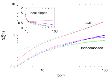
Figure 18: Analysis on the real space. Log-log plot of $S^{(2)}_{00}(r)$ versus $r$ (top curve), and of the three undecomposed longitudinal structure functions in the three directions $x,y,z$ (three bottom curves). The straight line gives the best fit slope $\zeta_{0}^{(2)}=0.7$. Inset: logarithmic local slopes of the same curves in the main body of the figure (same symbols). Notice that only the projected curve shows a nice plateau

Only for the projected correlation it is possible to measure (with $5\%$ of accuracy) the scaling exponent by a direct log-log fit versus the scale separation. The best fit gives $\zeta_{0}^{(2)}=0.70\pm 0.03$. On the contrary, the undecomposed structure functions are overwhelmed by the anisotropic effects present at all scales, and the scaling law is completely spoiled. We stress the accuracy of these results; already at these modest Reynolds numbers it is possible to ascertain the isotropic scaling laws if the anisotropic fluctuations are disentangled properly.

In figure 19 there is an overview for the second order structure functions in all the sectors, isotropic and anisotropic, for which the signal-to-noise ratio is high enough to ensure statistically stable results. Sectors with odd $j$ are absent due to the parity symmetry of the longitudinal structure function. We conclude from figure 19 a clear foliation in terms of the $j$ index : sectors with the same $j$ but different $m$ exhibit very close scaling exponents. In Table 3 the measured exponents are compiled, showing the best power law fits for structure functions of orders $n=2,4,6$.

Figure 19: Log-log plot of the second order structure function in all sectors with a strong signal. Symbols refer to sectors (j,m) as follows: $(0,0)$, ($+$); $(2,2)$, ($\times$); $(4,0)$, ($\Box$); $(4,2)$, ($\star$); $(6,0)$, ($\circ$); $(6,2)$, ($\blacksquare$). The statistical and numerical noise affecting the SO(3) projection is estimated as the threshold where the $j=6$ sector starts to deviate from the monotonic decreasing behavior, i.e. ${\mathcal{O}}(10^{-3})$

We stress again the discreteness and monotonicity of the scaling exponents as assumed in Eq. (180); there is no saturation of the exponents as a function of $j$. Second, the measured exponents in the sectors $j=4$ and $j=6$ are anomalous, i.e. they differ from the dimensional estimate given in 46.

$n$	$j=0$	$j=2$	$j=4$	$j=6$
	$\zeta_{0}^{(n)}$ — $n/3$	$\zeta_{2}^{(n)}$ — $(n+2)/3$	$\zeta_{4}^{(n)}$ — $(n+4)/3$	$\zeta_{6}^{(n)}$ — $(n+6)/3$
2	0.70 (2) — 0.66	1.1 (1) — 1.33	1.65 (5) — 2.00	3.2 (2) — 2.66
4	1.28 (4) — 1.33	1.6 (1) — 2.00	2.25 (10) — 2.66	3.1 (2) — 3.33
6	1.81 (6) — 2.00	2.1 (1) — 2.33	2.50 (10) — 3.33	3.3 (2) — 4.00

Table 3: Summary of the numerical and experimental findings for the scaling exponents in the isotropic and anisotropic sectors. The values for the anisotropic sector $j=2$ are taken from the experiments [10, 31]. For the values extracted from the numerical simulation (columns $j=0,4,6$), error bars are estimated from the oscillation of the local slopes [36, 139]. For the experimental data the error is given as the mismatch between the two experiments. For all sectors we also give the dimensional estimate $\zeta_{j}^{(n)}=(n+j)/3$ [15].

Unfortunately, from the RKF data it was not possible to obtain clean results for the $j=2$ sector. This is because of the presence of an annoying change of sign in the projections $S^{(n)}_{2m}(r)$ for any $m$ (and any order $n$). Still, the overall consistency of the foliation and hierarchical organization of scaling exponents can be checked by collecting the scaling exponents in the $j=2$ sector from the two sets of experiments [10, 31] previously discussed. In Fig. 20 we show both numerical data and the experimental values as extracted from [10, 31]. The resulting picture is fully coherent : experimental data coming from the $j=2$ sector fit well in the global trend. As one can see from table 3 all the anisotropic sectors show anomalous scaling laws.

Figure 20: Scaling exponents, $\zeta_{j}^{(n)}$, of structure functions of order $n=2,4,6$ for isotropic and anisotropic sectors. From the DNS of RKF we have : isotropic sector, $j=0$ ($+$); anisotropic sectors, $j=4$ ($\times$) and $j=6$ ($\star$). From the experimental data [10, 31], we have $j=2$ ($\Box$). For an estimate of error bars see Table 3.

7.2.1 Universality of Anisotropic Fluctuations

The third numerical experiment that we discuss here is devoted to study universal properties of anisotropic scaling. We have already commented that there is a nice qualitative and quantitative agreement between the values extracted for the $j=2$ sector (the only one available from experimental data) from different experiments. In order to check whether this universality holds also in higher anisotropic sectors one has to rely on DNS. In [131] a first direct comparison between anisotropic scaling of longitudinal structure functions from two different homogeneous systems, the RKF and a homogeneous Rayleigh-Bénard convective flow was reported.

A Homogeneous Rayleigh-Bénard system is a convective cell with fixed linear mean temperature profile along the vertical direction. The flow is obtained by decomposing the temperature field as the sum of a linear profile plus a fluctuating part, $T(x,y,z;t)=T^{\prime}(x,y,z;t)+(\Delta T/2-z\Delta T/H)$, where $H$ is the cell height and $\Delta T$ the background temperature difference. The evolution of the system can be described by a modified version [144] of the Boussinesq system [145]:

$$\partial_{t}\mbox{\boldmath$u$} + \left(\mbox{\boldmath$u$}\cdot\nabla\right)\mbox{\boldmath$u$}=-\nabla p+\nu\nabla^{2}\mbox{\boldmath$u$}+\alpha gT^{\prime}{{\mbox{\boldmath$\hat{z}$}}}$$

$$\partial_{t}T^{\prime} + \left(\mbox{\boldmath$u$}\cdot\nabla\right)T^{\prime}=\kappa\nabla^{2}T^{\prime}-{{\Delta T}\over H}v_{z}.$$

where $\alpha$ is the thermal expansion constant, $\nu$ and $\kappa$ the kinematic viscosity and the thermal diffusivity coefficients, and $g$ is the acceleration due to gravity. In [131] fully periodic boundary conditions were used for the velocity field, $u$, and temperature, $T^{\prime}$, fields.

Anisotropic effects in the Rayleigh-Bénard system were analyzed in [131] starting from the stationary equation for the second order velocity structure functions; the extension of Kármán-Howarth equation in the presence of a buoyancy term [146]. The result is, neglecting for simplicity tensorial symbols:

$$\langle\delta u({\bf r})^{3}\rangle \sim \ \ \bar{\epsilon}\ r\ +\ \alpha g{\mbox{\boldmath$\hat{z}$}}r\ \cdot\ \langle\delta T({\bf r})\ \delta u({\bf r})\rangle$$ (184)

_j=0,1,… $$\ \ {}_{j=0}\quad\ \ {}_{j=1\quad\otimes\quad j=1,2,\dots}$$

where $\bar{\epsilon}$ denotes the energy dissipation, $\langle\delta u({\bf r})^{3}\rangle$ and $\langle\delta T({\bf r})\ \delta u({\bf r})\rangle$, the general third-order velocity correlation and temperature-velocity correlation, respectively. In Eq. (184) for each term the value of its total angular momentum, $j$, is indicated. Notice that the energy dissipation term in (184) has a non-vanishing limit, for high Re, only in the isotropic sector, $j=0$. On the other hand, the buoyancy coupling, $\alpha g{\mbox{\boldmath$\hat{z}$}}$, brings only angular momentum $j=1$. Due to the usual rule of composition of angular momenta we have that the buoyancy term, $\alpha g{\mbox{\boldmath$\hat{z}$}}\cdot\langle\delta T({\bf r})\ \delta u({\bf r})\rangle$, has a total angular momentum given by: $j_{tot}=1\otimes j=\{j-1,j,j+1\}$. Using the angular momenta summation rule for $j$, one can decompose the previous equation obtaining the following dimensional matching, in the isotropic sector:

$$\langle\delta u(r)^{3}\rangle_{j=0}\sim\epsilon\ r+\alpha g\hat{{\bf z}}r\langle\delta u(r)\ \delta T(r)\rangle_{j=1}+\dots$$

and in the anisotropic sectors, $j>0$:

$$\langle\delta u(r)^{3}\rangle_{j}\sim\ \ \alpha g\ \hat{{\bf z}}r\ \langle\delta u(r)\ \delta T(r)\rangle_{(j-1)}+\dots$$ (185)

where sub-dominant contributions coming from the $j$ and $j+1$ sectors of $\langle\delta v(r)\ \delta T(r)\rangle$ are neglected.

In the isotropic sector the buoyancy term is sub-dominant with respect to the dissipation term at scales smaller than the Bolgiano length, $L_{B}=(\bar{\epsilon})^{5/4}N^{-3/4}(\alpha g)^{-3/2}$ where $N$ is the rate of temperature dissipation. This is the case for the numerical simulation presented in [131], where velocity fluctuations are closer to the typical Kolmogorov scaling, $\delta u(r)\sim r^{1/3}$, rather than to the Bolgiano-Obukhov scaling [1], $\delta u(r)\sim r^{3/5}$.
Regarding the anisotropic sectors, Eq.(185) is the dimensional prediction for the system, consistent with the anisotropic properties of the buoyancy term, sector by sector.
In [131] the SO(3) decomposition was applied in this system to velocity structure functions (44) and to objects

$$G^{(q,1)}({\bf r})=\langle\left[\left(\mbox{\boldmath$u$}\left({\bf r}\right)-\mbox{\boldmath$u$}\left(0\right)\right)\cdot{\mbox{\boldmath$\hat{r}$}}\right]^{q}\left(T\left({\bf r}\right)-T\left(0\right)\right)\rangle\,=\sum_{jm}G^{(q,1)}_{jm}(r)$$

The dimensional matching of Eq. (185) can be extended to any order, giving:

$$S^{(p)}_{jm}(r)\sim r{G}^{(p-2,1)}_{j-1,m}(r).$$

Denoting with $\chi_{j}^{(q,1)}$ the anisotropic scaling exponents of the buoyancy terms, ${G}^{(q,1)}_{jm}(r)\sim r^{\chi_{j}^{(q,1)}}$ we get the dimensional estimate:

$$\zeta_{j}^{(p)}=1+\chi_{j-1}^{(p-2,1)},\quad\mbox{ (dimensional prediction)}$$ (186)

In [131] it was shown that this dimensional prediction is not obeyed; the exponents $\zeta_{j}^{(n)}$ appear to be systematically smaller than the prediction (186). Interestingly, enough the log-log plots computed in the sectors $j=4,6$ show a good qualitative agreement with those calculated in the RKF of ref [36] as can be seen in fig. 21 where we compare the projection on the $j=4$ sector of structure functions of different orders.

Figure 21: Log-log plot of compensated anisotropic $j=4,m=0$ projections $S^{(p)}_{4,0}(r)/r^{\zeta_{4}^{(p)}}$ vs $r$, for both HRB and RKF flows. Top curves refer to $p=2$: the best fit exponents which compensate HRB and RKF curves are $\zeta_{4}^{(2)}=1.7$ and $\zeta_{4}^{(2)}=1.66$, respectively. Curves in the middle refer to the same quantities but for $p=4$: compensation has been obtained with $\zeta_{4}^{(4)}=2.05$ for HRB, and $\zeta_{4}^{(4)}=2.2$ for RKF. Bottom curves refer to $p=6$: here $\zeta_{4}^{(6)}=2.3$ for HRB, and $\zeta_{4}^{(6)}=2.5$ for RKF. Notice that the curves of the two flows are compensated with very similar values of the exponents (within $10\%$). Inset: the same but for $j=4,m=2$, compensation has been done with the same values used for $j=4,m=0$, to show the independence of the scaling exponents from the choice of the reference axis labeled with $m$ .

Similar results are obtained for $j=6$ sector. These preliminary findings, if confirmed by other independent measurements, would support universality for anisotropic scaling exponents in three dimensional turbulence.

7.3 Scaling of Longitudinal and Transversal structure functions

As discussed in Sect. 2.6 there exists experimental and numerical data suggesting that longitudinal and transversal structure functions in supposedly isotropic flows show different scaling exponents [30, 62, 63, 64, 65]. One needs to clearly distinguish between experimental and numerical data. The former can never be considered fully isotropic; the best one can do is to try to perform a multi-fit procedure to clean out sub-leading anisotropic contributions as already explained in details in Sect. 6. This fitting procedure is, of course, affected by experimental errors which cannot be eliminated. Therefore it is quite dangerous to make any firm conclusion about supposed different scaling exponents of longitudinal and transversal isotropic scaling on the basis of only experimental data . Numerical data are not much safer. Here anisotropy can be much better controlled. With isotropic forcing the only source of anisotropy is the 3-dimensional grid whose effect is usually too small to explain possible discrepancies between longitudinal and transversal scalings. Indeed some state-of-the-art isotropic DNS indicate the possibility of different scaling exponents both for inertial range structure functions [64] and for coarse grained energy and enstrophy measures [62, 147]. In Table 4 we summarize the best-fit values of the scaling exponents measured in [64]. The small scale fluctuations were probed [147] by comparing the scaling of the coarse grained energy dissipation over a box of size $r$, $\tilde{\epsilon}(r)$ (Eq. 17), and of the coarse grained enstrophy dissipation: $\omega(r,\mbox{\boldmath$x$})={1\over r^{3}}\int_{|y|<r}d\mbox{\boldmath$y$}~{}\omega(\mbox{\boldmath$x$}+\mbox{\boldmath$y$})$ where $\omega(\mbox{\boldmath$x$})$ is the local enstrophy dissipation. Different scaling exponents were measured for the averaged quantities, $\langle(\tilde{\epsilon})^{p}(r)\rangle$, $\langle\omega^{p}(r)\rangle$. Being scalar quantities one expects that in isotropic ensembles they would not have different exponents. From the theoretical point of view, different scaling exponents of longitudinal and transverse structure functions in isotropic ensembles are unlikely. In the language of the SO(3) decomposition it amounts to the scaling exponents depending on the $q$-index which labels different basis functions with the same rotation properties. In the exactly solvable models examined before, this had never happened. In general one would need a different symmetry to lift the degeneracy of different $q$ dependent basis functions. At this point this problem remains somehow unsettled. New numerical tests on larger grids and/or with a better resolved viscous behavior are needed before a firm statement can be made.

n	2	4	6	8	10
$\zeta^{(n)}_{0}$	0.701 (14)	1.29 (3)	1.77 (4)	2.17 (7)	2.53 (9)
$\zeta^{(n)}_{0}$	0.709 (13)	1.27 (2)	1.67 (4)	1.93 (9)	2.08 (18)

Table 4: Measured values of the longitudinal (first raw) and transverse (second raw) scaling exponents at $Re_{\lambda}=460$ taken from [64]. One should note that the scaling range displayed by the scaling plots in [64] are relatively short, indicating that finite Re effects may still be rather important

7.4 Anisotropies in decaying turbulence

Decaying turbulence has attracted the attention of various communities and is often considered in experimental, numerical and theoretical investigations [148, 5, 1]. It is in fact quite common that even experiments aimed at studying stationary properties of turbulence involve processes of decay. Important examples are provided by a turbulent flow behind a grid (see [149] and references therein) or the turbulent flow created at the sudden stop of a grid periodically oscillating within a bounded box [150]. In the former case, turbulence is slowly decaying going farther and farther away from the grid and its characteristic scale becomes larger and larger (see [149] for a thorough experimental investigation). Whenever there is sufficient separation between the grid-size $L_{in}$ and the scale of the tunnel or the tank $L_{0}\gg L_{in}$, a series of interesting phenomenological predictions can be derived. For example, the decay of the two-point velocity correlation function, for both isotropic and anisotropic flows, can be obtained under the so-called self-preservation hypothesis (see [1] chapter XVI). That posits the existence of rescaling functions allowing to relate correlation functions at different spatial and temporal scales. By inserting the rescaling function into the equations of motion, asymptotic results can be obtained both for the final viscosity-dominated regime and for the intermediate asymptotic when nonlinear effects still play an important role.

Here, we review some recent attempts to investigate the decay of three-dimensional homogeneous and anisotropic turbulence by direct numerical simulations of the Navier-Stokes equations in a periodic box [151] for both short and large times. The initial conditions are taken from the stationary ensemble of the Random Kolmogorov Flow discussed in the previous subsection. Here the correlation length-scale of the initial velocity field $L_{in}$ is of the order of the size of the box $L_{0}\approx L_{in}$.

On the one hand, one is interested in the long time decay regime where the typical interesting questions are: (i) how do global quantities, such as single-point velocity and vorticity correlations, decay? (ii) What is the effect of the outer boundary on the decay laws ? (iii) Do those quantities keep track of the initial anisotropy ? (iv) As for the statistics of velocity differences within the inertial range of scales, is there a recovery of isotropy at large times ? (v) If so, do strong fluctuations get isotropic at a faster/slower rate with respect to those of average intensity ? (vi) Do anisotropic -and isotropic- fluctuations decay self-similarly ? (vii)If not, do strong fluctuations decay slower or faster than typical ones ?  On the other hand, the interest in the early stages of the decay is led by a hope of establishing a link between the small-scale velocity statistics in this phase and in forced turbulence. If such links existed, they would shed additional light on the universality of forced turbulence. As turbulence decays, the effective Re decreases, while the viscous characteristic scale and time increase. In [151] an offline analysis at fixed multiples $\{0,1,10,10^{2},10^{3},10^{4},10^{5},10^{6}\}\,\tau_{0}$ of the initial large-scale eddy turnover time $\tau_{0}=L_{0}/u_{rms}^{t=0}$ was performed.
A first hint on the restoration of isotropy at large times can be extracted from the analysis of single point quantities as

$$E_{il}={\overline{u_{i}(\mbox{\boldmath$x$},t)u_{l}(\mbox{\boldmath$x$},t)}},\quad\Omega_{il}={\overline{\omega_{i}(\mbox{\boldmath$x$},t)\omega_{l}(\mbox{\boldmath$x$},t)}}.$$

Here with $\overline{\cdots}$ we denote the average over spatial coordinates only, whereas $\langle\cdots\rangle$ indicates the average over both initial conditions and space. The symmetric matrices $E_{il}(t)$ and $\Omega_{il}(t)$ can be diagonalized at each time-step and the eigenvalues $E_{1}(t),E_{2}(t),E_{3}(t)$ and $\Omega_{1}(t),\Omega_{2}(t),\Omega_{3}(t)$ can be extracted. The typical decay of $E_{i}(t)$ and $\Omega_{i}(t)$ for $i=1,\dots,3$ is shown in Fig. 22.

Figure 22: Log-log plot of the eigenvalues of energy and vorticity matrices vs. time, expressed in $\tau_{0}$ unit.

During the self-similar stage, $t\in[10,10^{6}]$, the energy eigenvalues fall off as $E_{\{1,2,3\}}\sim t^{-2}$, as expected for the decay in a bounded domain [149, 152]. The enstrophy eigenvalues, $\Omega_{\{1,2,3\}}$ decay as $t^{-12/5}$ as predicted from a simple dimensional argument [151]. To focus on the process of recovery of isotropy in terms of global quantities one may track the behavior of two sets of observables

$$\Delta_{il}E(t)=\frac{\langle E_{i}(t)-E_{l}(t)\rangle}{\langle E_{i}(t)+E_{l}(t)}\rangle\,,\quad\Delta_{il}{\Omega}(t)=\frac{\langle\Omega_{i}(t)-\Omega_{l}(t)\rangle}{\langle\Omega_{i}(t)+\Omega_{l}(t)\rangle}\,,$$

which vanish for isotropic statistics. Their rate of decay is therefore a direct measurement of the return to isotropy. The energy matrix $E_{il}$ is particularly sensitive to the large scales while small-scale fluctuations are sampled by $\Omega_{il}$. As seen from Fig. 23,

Figure 23: Log-log plot of the anisotropy content at the large scales ($\Delta_{12}E(t)$, $\Delta_{13}E(t)$, top curves) and the small scales ($\Delta_{12}\Omega(t)$, $\Delta_{13}\Omega(t)$, bottom curves) as a function of time, expressed in $\tau_{0}$ unit. The large-scale (small-scale) anisotropy content is defined as the mismatch between the eigenvalues of the single-point velocity (vorticity) correlation.

both large and small scales begin to isotropize after roughly one eddy turnover time and become fully isotropic (within statistical fluctuations) after $100$ eddy turnover times. However, small scales show an overall degree of anisotropy much smaller than the large scales.

Concerning small scales properties, in [151] a simple anisotropic generalization of the self-preservation hypothesis (see, e.g. Ref. [5]) was proposed:

$$S^{(n)}_{jm}\left(r,t\right)=V^{(n)}_{jm}\left(t\right)f^{(n)}_{jm}\left(r/L_{jm}(t)\right).$$

Here with $V^{(n)}_{jm}\left(t\right)$ we take explicitly into account the fact that large-scale velocity properties may depend in a nontrivial way on both $(j,m)$ and the order $n$. Furthermore, $L_{jm}(t)$ accounts for the possibility that the characteristic length scale depend on the SO(3) sector. In analogy with the observations made in the stationary case [55, 29, 34, 10, 36, 15, 30, 35] a scaling law was postulated:

$$S^{(n)}_{jm}\left(r,t\right)\sim a^{(n)}_{jm}(t)\left(\frac{r}{L_{jm}(t)}\right)^{\zeta_{j}^{(n)}}\,.$$ (187)

The time behavior is encoded in both the decay of the overall intensity, accounted by the prefactors $a^{(n)}_{jm}(t)$, and the variation of the integral scales $L_{jm}(t)$. The representation Eq. (187) is the simplest one fitting the initial time statistics for $t=0$ and agreeing with the evolution given by the self preservation hypothesis in the isotropic case. The power law behavior for $f^{(n)}_{jm}\left(r/L_{jm}(t)\right)$ can be expected only in a time-dependent inertial range of scales $\eta(t)\ll r\ll L(t)$. As for the exponents appearing in (187), their values are expectedly the same as in the stationary case. Concerning the time evolution, it seems difficult to disentangle the dependence due to the decay of $a^{(n)}_{jm}(t)$ from the one due to the growth of the integral scale $L_{jm}(t)$. The existence of a running reference scale, $L_{jm}(t)$ introduces some non-trivial relations between the spatial anomalous scaling and the decaying time properties, and those relations might be subject to experimental verification. In the case discussed in [151], the fact that the initial condition has a characteristic length-scale comparable with the box size, simplifies the matter. Indeed we expect that $L_{jm}(t)\approx L_{0}$, and the decay is due only to the fall-off of $a^{(n)}_{jm}(t)$. An obvious shortcoming is that the width of the inertial range $L_{0}/\eta(t)$ shrinks monotonically in time, thereby limiting the possibility of precise quantitative statements.

7.4.1 Long time decay

A quantitative way to define the temporal rate of recovery of isotropy at a fixed scale in the inertial range is given by the dimensionless ratio:

$$\Pi^{(n)}_{jm}\left(r,t\right)\equiv\frac{S^{(n)}_{jm}\left(r,t\right)}{S^{(n)}_{0,0}\left(r,t\right)}\sim t^{-\Xi_{j}^{(n)}}\,.$$ (188)

In Fig. 24,

Figure 24: Hierarchical organization of anisotropic fluctuations at long times. Log-log plot of the anisotropic projections normalized by the corresponding isotropic projection (see text), at two fixed scales $r=80$ and $r=40$ (inset) for $n=2,4,6$ in the anisotropic sector $j=4,m=0$. Symbols read as follows : $\Pi^{(2)}_{40}$ (full box); $\Pi^{(4)}_{40}$ (star); $\Pi^{(6)}_{40}$ (empty box). The straight line is $t^{-\Xi}$ with $\Xi\sim 0.3$. Same symbols in the inset.

we plot $\Pi^{(n)}_{jm}\left(r,t\right)$ at $r=80$ for structure functions of order $n=2,4,6$ and for the most intense anisotropic sector, $(j,m)=(4,0)$. All anisotropic sectors, for all measured structure functions, decay faster than the isotropic one. The measured slope in the decay is about $\Xi_{j}^{(n)}\sim 0.3$ for all $n$, within the statistical errors. Note that these results agree with the simple picture that the time-dependence in (187) is entirely carried by the prefactors $a_{jm}^{(n)}(t)$ and the value of the integral scales $L_{jm}(t)$ is saturated at the size of the box. Indeed, by assuming that large-scale fluctuations are almost Gaussian we have that the leading time-dependence of $a_{jm}^{(2n)}$ is given by $a_{jm}^{(2)}a_{00}^{(2n-2)}$. For the isotropic sector, $a_{00}^{(2n)}\sim(a_{00}^{(2)})^{n}$, and plugging that in (188), one get: $\Pi^{(n)}_{jm}\left(r,t\right)\sim a^{(2)}_{jm}(t)/a^{(2)}_{00}(t)\sim t^{-\Xi}$ with $\Xi\sim 0.3(\pm 0.1)$ independent of $n$. The quality of data is insufficient to detect possible residual effects due to $L_{jm}(t)$, which would make $\Xi_{j}^{(n)}$ depend on $n$ and $j$ because of spatial intermittency.

Let us denote with ${\mathcal{P}}(\Delta,{\bf r};t)$ the probability to observe a given longitudinal fluctuation, $\delta u_{\ell}(\mbox{\boldmath$r$},t)=\Delta$ in the direction ${\bf r}$ at a given time, $t$. For any given fixed value $\Delta$ and for any given time, $t$, we can project ${\mathcal{P}}(\Delta,{\bf r};t)$ on the SO(3) basis functions:

$${\mathcal{P}}(\Delta,{\bf r};t)=\sum_{j=0}^{\infty}\sum_{m=-j}^{j}{\mathcal{P}}_{jm}\left(r,\Delta;t\right)Y_{jm}({\mbox{\boldmath$\hat{r}$}}),$$ (189)

where now the projection, ${\mathcal{P}}_{jm}\left(r,\Delta;t\right)$ play the role of an effective PDF for each SO(3) sector. The projection of any longitudinal structure function, $S^{(n)}({\bf r},t)$ on any sector, $(j,m)$ can be reconstructed from the corresponding projection of the PDF on the same sector, ${\mathcal{P}}_{jm}\left(r,\Delta;t\right)$, by averaging over all possible $\Delta$:

$$S^{(n)}_{jm}\left(r,t\right)=\int d\Delta\Delta^{n}{\mathcal{P}}_{jm}\left(r,\Delta;t\right)$$

which establish the link between decomposition (44) and (189).

The interesting fact that the decay properties of the anisotropic sectors are almost independent of $n$ indicates that a non-trivial time dependence in the shape of the PDF’s ${\mathcal{P}}_{jm}\left(r,\Delta;t\right)$ for $j>0$ must be expected. The most accurate way to probe the rescaling properties of ${\mathcal{P}}_{jm}\left(r,\Delta;t\right)$ in time is to compute the generalized flatness:

$$K_{jm}^{(n)}(r,t)\equiv\frac{S^{(n)}_{jm}\left(r,t\right)}{\left(S^{(2)}_{jm}\left(r,t\right)\right)^{\frac{n}{2}}}\sim t^{\alpha_{j}^{(n)}}$$

Were the PDF projection in the $(j,m)$ sector self-similar for $t\gg\tau_{0}$, then $K_{jm}^{(n)}(r,t)$ would tend to constant values. This is not the case for anisotropic fluctuations, as it is shown in Fig. (25).

Figure 25: Log-log plot of the generalized flatness, $K_{jm}^{(n)}(r,t)$ of order $n=4,6$ for both the isotropic (two bottom curves), and the anisotropic sector $(j=4,m=0)$ (two top curves) at $r=80$, and as a function of time. In the inset we plot the same quantities, in the same order, at a different inertial range scale, $r=40$.

The curves $K_{jm}^{(n)}(r,t)$ are collected for two fixed inertial range separations, $r=80$ and $r=40$ (inset), for two different orders, $n=4,6$ and for both the isotropic and one of the most intense anisotropic sectors $(j=4,m=0)$ . The isotropic flatness tends toward a constant value for large $t$. Conversely, its anisotropic counterparts are monotonically increasing with $t$, indicating a tendency for the anisotropic fluctuations to become more and more intermittent as time elapses. Also the behavior in Fig. 25 is in qualitative agreement with the observation previously made that all the time dependence can be accounted for by the prefactors $a_{jm}^{(n)}(t)$. Indeed, assuming that the length scales $L_{jm}(t)$ have saturated and that the large scale PDF is close to Gaussian, it is easy to work out the prediction $K_{jm}^{(n)}(r,t)\sim t^{-\Xi(1-n/2)}$, i.e. $\alpha_{j}^{(n)}=\Xi(n/2-1)$. We conclude this section by a brief summary of the results. It was found that isotropic fluctuations persist longer than anisotropic ones, i.e. there is a time-recovery, albeit slower than predicted by dimensional arguments, of isotropy during the decay process. It was also found that isotropic fluctuations decay in an almost self-similar way while the anisotropic ones become more and more intermittent. Qualitatively, velocity configurations get more isotropic but anisotropic fluctuations become, in relative terms, more “spiky” than the isotropic ones as time elapses.

7.4.2 Short-time decay

It is interesting to notice that it is possible to relate the small-scale universal properties of forced turbulent statistics to those of short-time decay for an ensemble of initial configurations [151]. As already remarked, one cannot expect an universal behavior for all statistical observables, as the very existence of anomalous scaling is the signature of the memory of the boundaries and/or the external forcing throughout all the scales. Indeed, the main message we want to convey here is that only the scaling exponents of both isotropic and anisotropic small-scale fluctuations are universal, at least for forcing concentrated at large scales. The prefactors are not expected to be so. There is therefore no reason to expect that quantities such as the skewness, the kurtosis and in fact the whole PDF of velocity increments or gradients be universal.
This is the same situation that we discussed in great details in previous sections for the passive transport of scalar and vector fields. However, carrying over the analytical knowledge developed for linear hydrodynamic problems involve some nontrivial, yet missing, steps. For the Navier-Stokes dynamics, linear equations of motion appear when we consider the whole set of correlation functions as discussed in Sect. 4.3. These equations can be rewritten in a schematic form:

$$\partial_{t}C^{(n)}=\Gamma^{(n+1)}C^{(n+1)}+\nu D^{(n)}C^{(n)}+F^{(n)},$$ (190)

where $\Gamma^{(n+1)}$ is the integro-differential linear operator coming from the inertial and pressure terms, $C^{(n)}$ is a shorthand notation for a generic $(n)$-th order correlator and $D^{(n)}$ is the linear operator describing dissipative effects. Finally, $F^{(n)}$ is the correlator involving increments of the large-scale forcing $f$ and of the velocity field. The balance between inertial and injection terms cannot lead to anomalous scaling. A natural possibility is that a mechanism similar to the one identified in linear transport problems be at work in the Navier-Stokes case as well. The anomalous contributions to the correlators would then be associated with statistically stationary solutions of the unforced equations (190). The scaling exponents would a fortiori be independent of the forcing and thus universal. As for the prefactors, the anomalous scaling exponents are positive and thus the anomalous contributions grow at infinity. They should then be matched at the large scales with the contributions coming from the forcing to ensure that the resulting combination vanish at infinity, as required for correlation functions. The aim here is not to prove the previous points but rather to test whether they fail: the Navier-Stokes equations, being integro-differential and non-local, might directly couple inertial and injection scales and spoil the argument. This effect might be particularly relevant for anisotropic fluctuations where infrared divergences may appear in the pressure integrals (see Sect. 5.3). In order to investigate the previous point, we performed two sets of numerical experiments in decay.

The first set, A, is of the same kind as in the previous section, i.e. we integrated the unforced Navier-Stokes equations with initial conditions picked from an ensemble obtained from a forced anisotropic stationary run. Statistical observables are measured as an ensemble average over the different initial conditions. The ensemble at the initial time of the decay process therefore coincides with the stationary state in forced runs. If correlation functions are indeed dominated at small scales by statistically stationary solutions of the unforced equations then the field should not decay. Specifically, the field should not vary for times smaller than the large-scale eddy turnover time $\tau_{0}$. Those are the times when the effects of the forcing terms start to be felt. Note that this should hold at all scales, including the small ones whose turnover times are much faster than $\tau_{0}$.

The second set of numerical simulations (set B) takes the same initial conditions but for the random scrambling of the phases : $\mbox{\boldmath$u$}_{i}({\bf k})\rightarrow P_{il}({\bf k})\mbox{\boldmath$u$}_{l}({\bf k})\exp(i\theta_{l}({\bf k}))$, with $\theta_{l}({\bf k})$ i.i.d. random variables. In this way, the spectrum and its scaling exponent are preserved but the wrong organization of the phases is expected to spoil the statistical stationarity of the initial ensemble. As a consequence, two different decays are expected for the two sets of initial conditions. In particular, contrary to set A, set B should vary at small scales on times of the order of the eddy turnover times $\tau_{r}\sim r^{2/3}$. This is exactly what has been found in the numerical simulations for both isotopic and anisotropic statistics as can be seen for the anisotropic case in Fig. 26,

Figure 26: Top: Temporal decay of the second-order anisotropic structure function $S^{(2)}_{40}(r,t)$, rescaled by its value at $t=0$. Here $r=30$, inside the inertial range. The two curves refer to the time evolution of the structure function starting from the forced-stationary velocity fields (squares, set A) and from the randomly dephased velocity fields (circles, set B). Time is normalized by the integral eddy turnover time. Notice that for set B we observe changes on a time scale faster than the integral eddy turnover time. That is to be contrasted with the case A, where structure functions are strictly constant in time up to an integral eddy turnover time. Bottom: The same curves but for the fourth-order structure function.

where the temporal behavior of longitudinal structure functions of order 2 and 4 is shown. The scaling exponents of the contributions responsible for the observed behavior at small scales are thus forcing independent.
To conclude, the data presented here support the conclusion that nonlocal effects peculiar to the Navier-Stokes dynamics do not spoil arguments on universality based on analogies with passive turbulent transport. The picture of the anomalous contributions to the correlation functions having universal scaling exponents and non-universal prefactors follows.

8 Concluding Discussion,

In this review we presented a mathematical framework in which anisotropy in turbulence can be studied, and we have tested its utility in the context of experimental analysis, numerical simulations and analytical models. The basic idea is to express the various statistical quantities of turbulence (e.g., structure functions, correlation functions) in terms of their projections on the different sectors of the SO($3$) group.

The utility of the SO($3$) decomposition should be assessed in two main aspects. The first aspect is its functionality as a tool for characterizing anisotropy, whereas the second, and deeper aspect, is its physical relevance and the theoretical and analytical advantages that are gained by using it.

As a tool for describing anisotropy, the SO($3$) decomposition is probably the most natural and general method. It is of high resolution - it subdivides the observed anisotropy into different sectors - the $(j,m)$ sectors. The weights of the various sectors give us a fine resolution of the anisotropy structure. Instead of having one measure for anisotropy (e.g., the overall percentage of anisotropy), we have an infinite set of numbers that compose a detailed profile of the anisotropy structure.

The SO($3$) decomposition is also very general. It is applicable to any physical observable that has a well-defined transformation under rotations. These can be, for example, correlation functions, structure functions or Green’s functions (response functions). The observables themselves may depend on any number of space coordinates or even be space independent. They may also be scalars, vectors or tensors. Any such quantity can be presented as a sum of parts that belong to the different $(j,m)$ sectors of the rotation group. Additionally, since the SO($3$) decomposition is invariant to isotropic operations, it is invariant to the most common operations that we use. For example, to obtain the $n$th order longitudinal structure function we can take the full $n$th order structure function (which is a tensor) and contract it with $n$ unit vectors in the direction of the separation distance. Since this operation is linear and isotropic, it will preserve the $(j,m)$ sectors of the full structure function. That is, the $(j,m)$ sector of the full structure function will be transformed into the same $(j,m)$ sector of the longitudinal structure functions. The same thing happens for operations such as differentiations (for example when we look at moments of the gradient fields), space averaging, time averaging, coordinate fusion etc… From the pure theoretical point of view the first and most obvious advantage of using the SO($3$) decomposition is its elegance and the overwhelming simplification that it offers in analytical calculations. The SO($3$) decomposition may also have a deeper physical justification if it produces universal quantities such as distinct scaling behavior in the anisotropic sectors. There are several different evidences that suggest that this is indeed the case. Experimental results clearly show that a better scaling is achieved if we take higher $j$ components into account. Additionally, different experimental setups seem to lead to the same numerical values of the anisotropic exponent. This is a strong support for the hypothesis that the anisotropic sectors of the structure functions have universal exponents. Another support for the idea that the SO($3$) decomposition exposes universal quantities, comes from numerical simulations. In DNS, the SO($3$) decomposition can be performed directly (since the velocity field is accessible in every point in space and time) which makes the results much less ambiguous. We clearly see that even in the very moderate Reynolds numbers of the simulations, a scaling behavior is detected once we use the SO($3$) decomposition. In some cases, without the SO($3$) decomposition no scaling behavior is seen at all. Furthermore, the resulting exponents in the isotropic sector are remarkably similar to the experimental values which are measured at very high Reynolds numbers. This is a strong indication that at least the isotropic sector has a universal profile, and therefore by disentangling it from the anisotropic sectors we get universal results. In other sectors of the rotation group, the scaling behavior is not as good, and in some sectors there is no scaling at all. However, in those sectors where scaling was detected, the scaling exponents seem to agree with the theoretical and experimental predictions. Sectors with same $j$ and different $m$s had the same scaling exponents (when scale-invariance was observed). And finally, all exponents increased as a function of $n$ (order of the structure-function) as well as $j$. It is still not clear whether the “bad”, non scale-invariant behavior that was detected in some sectors, is a result of the poor Reynolds numbers of the simulations, or is a genuine effect that tells us that the foliation picture is incomplete. A further research with higher resolution is probably needed to settle this issue. In the Navier-Stokes case one can prove a “weak foliation”. Weak foliation is an approximate foliation that happens in the case of weak anisotropy, when we linearize the anisotropic part of the theory around its isotropic part. In such case, the linearized anisotropic part of the theory is subject to a linear and isotropic equation whose kernel contains the isotropic solution, and hence foliation occurs. This is a very robust approximation since it holds for virtually any nonlinear and isotropic theory in the case of weak anisotropy. Additionally, we know that as the Reynolds number increases, the statistics becomes more and more isotropic and therefore the linear approximation becomes better and better.

The SO($3$) decomposition has a physical relevance also in the presence of strong anisotropy. If we merely consider the direct application of the Navier-Stokes and continuity equations on the various structure functions, we get a family of linear and isotropic constraints. These constraints are valid independently of the amount of anisotropy in the system. Their linearity and isotropy lead to foliation and hence one can discuss them in every sector independently. In some sectors, they are sufficient to determine the full solution, whereas in others they can reveal some general properties of the solution. For example, the isotropic sector of the third-order structure function is completely determined by the different constraints, and is given by the well-known 4/5 law of Kolmogorov. Notice that because of foliation, this is true also in the presence of anisotropy, which means that the 4/5 law holds also in an anisotropic turbulence. In the $j=2$ sectors, on the other hand, the third-order structure-function is given by two undetermined scalar functions, whereas in the $j=4,6,\ldots$ it is given by three. Another example is the $j=1$ sectors in the second-order correlation function, which must all vanish.

To conclude, the framework of the SO($3$) decomposition provides an elegant and efficient way to describe anisotropy in turbulence. It also greatly simplifies many analytical calculations that involve anisotropic quantities, mainly through the mechanism of foliation. This mechanism is present in simplified models of turbulence, and may also be valid approximately in Navier-Stokes turbulence. It predicts that the anisotropic sectors of the statistics have universal properties such as scaling exponents. Further research is needed to accurately measure these anisotropic exponents in experiments as well as in numerical simulations.

A quantitative computation of the anisotropic exponents in Navier-Stokes turbulence from first principles may very well be an illusive goal. Nevertheless, we believe that the general principles of the physics behind these exponents and anisotropy in general can be understood.

9 Acknowledgements

We benefited from many discussion with many colleagues, without which we could not reach the picture presented in this review. We thank in particular Itai Arad, Roberto Benzi, Guido Boffetta, Carlo Casciola, Antonio Celani, Isabelle Daumont, Siegfried Grossmann, Boris Jacob, Susan Kurien, Alessandra Lanotte, Detlef Lohse, Victor S. Lvov, Irene Mazzitelli, Evgeny Podivilov, K.R. Sreenivasan, Federico Toschi and Massimo Vergassola. Much of the work reviewed here was supported in part by the European Commission through a TMR grant (No. HPRN-CT 2000-00162), the Italian Ministry of Education (MURST), the Instituto Nazionale di Fisica della Materia, the German Israeli Foundation, the Minerva Foundation, Munich, Germany, the Israel Science Foundation, and the US Israel Bi-National Science Foundation.

Appendix A The General Form of the 2nd Rank Tensor

In this appendix we discuss the general structure of the second rank correlation functions

$$F^{\alpha\beta}({\bf r})\equiv\langle u^{\alpha}({\bf x}+{\bf r})u^{\beta}({\bf x})\rangle\ ,$$ (191)

In (191) homogeneity of the flow is assumed, but not isotropy. Note that this object is more general than the structure function $S^{\alpha\beta}$ in being nonsymmetric in the indices, and having no definite parity. We wish to find the basis functions $B_{q,jm}^{\alpha\beta}({\bf\hat{r}})$, with which we can represent $F^{\alpha\beta}({\bf r})$ in the form:

$$F^{\alpha\beta}({\bf r})=\sum_{q,jm}a_{q,jm}(r)B_{q,jm}^{\alpha\beta}({\bf\hat{r}})$$ (192)

and derive some constraints among the functions $\ a_{q,jm}(r)$ that result from incompressibility. We shall see, that due to the isotropy of the incompressibility conditions, the constraints are among $a_{q,jm}(r)$ with the same $j,m$ only.

We begin by analyzing the incompressibility condition: An incompressible flow with constant density is characterized by the relation: $\partial_{\alpha}u^{\alpha}({\bf x},t)=0$ as a result, one immediately gets the following constraints on $F^{\alpha\beta}({\bf r})$:

$$\partial_{\alpha}F^{\alpha\beta}({\bf r})=0,\qquad\partial_{\beta}F^{\alpha\beta}({\bf r})=0.$$

Plugging the trial tensor (192) into the last two equations we obtain 2 equations connecting the different $a_{q,jm}$:

$$\partial_{\alpha}\sum_{q,jm}a_{q,jm}(r)B_{q,jm}^{\alpha\beta}({\bf\hat{r}})=0\qquad\partial_{\beta}\sum_{q,jm}a_{q,jm}(r)B_{q,jm}^{\alpha\beta}({\bf\hat{r}})=0$$ (193)

We first notice that the differentiation action is isotropic. As a result, if $T^{\alpha\beta}\left({\bf r}\right)$ is some arbitrary tensor with a definite $j,m$ transformation properties, then the tensor $\partial_{\alpha}T^{\alpha\beta}({\bf r})$ will have the same $j,m$ transformation properties. Components with different $j,m$ are linearly independent. Therefore equations (193) should hold for each $j,m$ separately.

Next, we observe that (193) are invariant under the transformation $F^{\alpha\beta}\longrightarrow F^{\beta\alpha}$. As a result, the symmetric and anti-symmetric parts of $F^{\alpha\beta}$ should satisfy (193) independently. To see that, let us write $F^{\alpha\beta}$ as a sum of a symmetric term and an anti-symmetric term: $F^{\alpha\beta}=F_{S}^{\alpha\beta}+F_{A}^{\alpha\beta}$, we then get:

$$\partial_{\alpha}F^{\alpha\beta} = \partial_{\alpha}F_{S}^{\alpha\beta}+\partial_{\alpha}F_{A}^{\alpha\beta}=\partial_{\alpha}F_{S}^{\beta\alpha}-\partial_{\alpha}F_{A}^{\beta\alpha}=0$$

$$\partial_{\beta}F^{\alpha\beta} = \partial_{\beta}F_{S}^{\alpha\beta}+\partial_{\beta}F_{A}^{\alpha\beta}=0$$

from which we conclude:$\partial_{\alpha}F_{S}^{\alpha\beta}=\partial_{\alpha}F_{A}^{\alpha\beta}=0.$ Finally, (193) is invariant under the transformation $F^{\alpha\beta}({\bf r)}\longrightarrow F^{\alpha\beta}(-{\bf r)}$ and as a result the odd parity and the even parity parts of $F^{\alpha\beta}$ should fulfill (193) independently. We conclude that a necessary and sufficient condition for (193) to hold is that it holds separately for parts with definite $j,m$, definite symmetry in the $\alpha,\beta$ indices and a definite parity in ${\bf r}$:

$$\partial_{\alpha}\sum_{q}a_{q,jm}({r})B_{q,jm}^{\alpha\beta}({\bf\hat{r}})=0\mbox{ \ \begin{tabular}[]{l}~{}~{}{\small summation is over}\\ ~{}~{}$B_{q,jm}^{\alpha\beta}$ {\small with definite symmetries}\end{tabular} }$$

where the summation is over $q$ such that $B_{q,jm}^{\alpha\beta}$ has a definite indices symmetry and a definite parity.

According to (37) we can write these $B_{q,jm}^{\alpha\beta}$ as:

1. $(-)^{j}$ parity, symmetric tensors:

   • $B_{1,jm}^{\alpha\beta}(\hat{{\bf r}})\equiv r^{-j}\delta^{\alpha\beta}\Phi_{jm}($$r$$)$,

   • $B_{7,jm}^{\alpha\beta}(\hat{{\bf r}})\equiv r^{-j}\left[r^{\alpha}\partial^{\beta}+r^{\beta}\partial^{\alpha}\right]\Phi_{jm}($$r$ $)$,

   • $B_{9,jm}^{\alpha\beta}(\hat{{\bf r}})\equiv r^{-j-2}r^{\alpha}r^{\beta}\Phi_{jm}($$r$$)$,

   • $B_{5,jm}^{\alpha\beta}(\hat{{\bf r}})\equiv r^{-j+2}\partial^{\alpha}\partial^{\beta}\Phi_{jm}($$r$$)$.

2. $(-)^{j}$ parity, anti-symmetric tensors:

   • $B_{3,jm}^{\alpha\beta}(\hat{{\bf r}})\equiv r^{-j}\left[r^{\alpha}\partial^{\beta}-r^{\beta}\partial^{\alpha}\right]\Phi_{jm}($$r$ $)$.

3. $(-)^{j+1}$ parity, symmetric tensors

   • $B_{8,jm}^{\alpha\beta}(\hat{{\bf r}})\equiv r^{-j-1}\left[r^{\alpha}\epsilon^{\beta\mu\nu}r_{\mu}\partial_{\nu}+r^{\beta}\epsilon^{\alpha\mu\nu}r_{\mu}\partial_{\nu}\right]\Phi_{jm}($$r$$)$,

   • $B_{6,jm}^{\alpha\beta}(\hat{{\bf r}})\equiv r^{-j+1}\left[\epsilon^{\beta\mu\nu}r_{\mu}\partial_{\nu}\partial^{\alpha}+\epsilon^{\alpha\mu\nu}r_{\mu}\partial_{\nu}\partial^{\beta}\right]\Phi_{jm}($$r$$)$.

4. $(-)^{j+1}$ parity, anti-symmetric tensors:

   • $B_{4,jm}^{\alpha\beta}(\hat{{\bf r}})\equiv r^{-j-1}\epsilon^{\alpha\beta\mu}r_{\mu}\Phi_{jm}($$r$$)$,

   • $B_{2,jm}^{\alpha\beta}(\hat{{\bf r}})\equiv r^{-j+1}\epsilon^{\alpha\beta\mu}\partial_{\mu}\Phi_{jm}($$r$$)$.

In order to differentiate these expressions we can use the following identities:

$$r^{\alpha}\partial_{\alpha}r^{\zeta}Y_{jm}(\hat{{\bf r}}) = \zeta r^{\zeta}Y_{jm}(\hat{{\bf r}})\ ,$$

$$\partial^{\alpha}\partial_{\alpha}r^{\zeta}Y_{jm}(\hat{{\bf r}}) = \left[\zeta\left(\zeta+1\right)-j(j+1)\right]r^{\zeta-2}Y_{jm}(\hat{x})$$

which give rise to:

$$r^{\alpha}\partial_{\alpha}\Phi_{jm}({\bf r}) = j\Phi_{jm}({\bf r})\ .$$

$$\partial^{\alpha}\partial_{\alpha}\Phi_{jm}({\bf r}) = 0\ .$$

From this point, it is a matter of simple (though somewhat lengthy) algebra to derive the differential constraints among $a_{q,jm}(r)$. The results are as follows:

1. $q\in\{1,7,9,5\}$

   $$a {}_{1,jm}^{\prime}(r)-jr^{-1}a_{1,jm}+ja_{7,jm}^{\prime}-j^{2}r^{-1}a_{7,jm}+a_{9,jm}^{\prime}+2r^{-1}a_{9,jm}=0\ ,$$

   $$r {}^{-1}a_{1,jm}+a_{7,jm}^{\prime}+3r^{-1}a_{7,jm}+\left(j-1\right)a_{5,jm}^{\prime}-\left(j^{2}-3j+2\right)r^{-1}a_{5,jm}=0\ .$$

2. $q\in\{3\}$

   $$a_{3,jm}^{\prime}-jr^{-1}a_{3,jm} = 0\ ,$$ (195)

   $$a_{3,jm}^{\prime}+r^{-1}a_{3,jm} = 0\ .$$

   These equations have no solutions other than: $a_{3,jm}(r)=0$.

3. $q\in\{8,6\}$

   $$a_{8,jm}^{\prime}+3r^{-1}a_{8,jm}+(j-1)a_{6,jm}^{\prime}-\left(j^{2}-2j+1\right)r^{-1}a_{6,jm}=0\ .$$ (196)

4. $q\in\{4,2\}$

   $$r^{-1}a_{4,jm}-a_{2,jm}^{\prime}+(j-1)r^{-1}a_{2,jm}=0\ .$$ (197)

There are obviously more unknowns than equations, since we merely exploited the incompressibility conditions. Nevertheless, we believe that the missing equations that arise from the dynamical hierarchy of equations will preserve the distinction between $a_{q,jm}$ of different $j,m$ (again, due to the isotropy of these equations). Note also, that the above analysis holds also for the second-order structure function

$$S^{\alpha\beta}({\bf r})\equiv\left\langle\left[u^{\alpha}({\bf x}+{\bf r})-u^{\alpha}({\bf x})\right]\left[u^{\beta}({\bf x}+{\bf r})-u^{\beta}({\bf x})\right]\right\rangle.$$

Only that in this case we should only consider the representations $q=1,7,9,5$ for even $j$ and the representations $q=8,6$ for odd $j$. This follows from the fact that $S^{\alpha\beta}({\bf r})$ is symmetric with respect to its indices and it has an even parity in  ${\bf r}$. Also, in that case, it is possible to go one step further by assuming a specific functional form for the $a_{q,jm}(r)$. We know that the $S^{\alpha\beta}({\bf r})$ is expected scale in the inertial range, and we therefore may assume:

$$a_{q,jm}(r)\equiv c_{q,jm}r^{\zeta_{2}^{(j)}}.$$

where $c_{q,jm}$ are just numerical constants. If we now substitute this definition into the equations (1,196), we get a set of linear equations among the $c_{q,jm}$. These relations can be easily solved and give us two possible tensors for even $j$ ($q=1,7,9,5$) and one tensor form for odd $j$ (from $q=8,6$). This kind of approach was taken in the two-probes experiment which is described in Sect. 6.

Appendix B Anisotropy in d-dimensions

To deal with anisotropy in d-dimensions we need classify the irreducible representations of the group of all $d$-dimensional rotations, SO(d) [153], and then to find a proper basis for these representations. The main linear space that we work in (the carrier space) is the space of constant tensors with $n$ indices. This space possesses a natural representation of SO(d), given by the well known transformation of tensors under $d$-dimensional rotation.

The traditional method to find a basis for the irreducible representations of SO(d) in this space, is using the Young tableaux machinery on the subspace of traceless tensors [153, 154]. It turns out that in the context of the present work, we do not need the explicit structure of these tensors. Instead, all that matters are some relations among them. A convenient way to derive these relations is to construct the basis tensors from functions on the unit $d$-dimensional sphere which belong to a specific irreducible representation. Here also, the explicit form of these functions in unimportant. All that matters for the calculations is the action of the Laplacian operator on these functions.

Let us therefore consider first the space $\mathcal{S}_{d}$ of functions over the unit $d$-dimensional sphere. The representation of SO(d) over this space is naturally defined by:

$$\mathcal{O}_{\mathcal{R}}\Psi(\hat{u})\equiv\Psi({\mathcal{R}}^{-1}\hat{u})\ ,$$ (198)

where $\Psi(\hat{u})$ is any function on the $d$-dimensional sphere, and ${\mathcal{R}}$ is a $d$-dimensional rotation.

${\mathcal{S}}_{d}$ can be spanned by polynomials of the unit vector $\hat{u}$. Obviously (198) does not change the degree of a polynomial, and therefore each irreducible representation in this space can be characterized by an integer $j=0,1,2,\ldots$, specifying the degree of the polynomials that span this representation. At this point, we cannot rule out the possibility that some other integers are needed to fully specify all irreducible representations in ${\mathcal{S}}_{d}$ and therefore we will need below another set of indices to complete the specification.

We can now choose a basis of polynomials $\{Y_{j,\sigma}(\hat{u})\}$ that span all the irreducible representations of SO(d) over ${\mathcal{S}}_{d}$. The index $\sigma$ counts all integers other than $j$ needed to fully specify all irreducible representations, and in addition, it labels the different functions within each irreducible representation.

Let us demonstrate this construction in two and three dimensions. In two dimensions $\sigma$ is unneeded since all the irreducible representation are one-dimensional and are spanned by $Y_{j}(\hat{u})=e^{ij\phi}$ with $\phi$ being the angle between $\hat{u}$ and the the vector $\hat{e}_{1}\equiv(1,0)$. Any rotation of the coordinates in an angle $\phi_{0}$ results in a multiplicative factor $e^{i\phi_{0}}$. It is clear that $Y_{j}(\hat{u})$ is a polynomial in $\hat{u}$ since $Y_{j}(\hat{u})=[\hat{u}\cdot\hat{p}]^{j}$ where $\hat{p}\equiv(1,i)$. In three dimensions $\sigma=m$ where $m$ takes on $2j+1$ values $m=-j,-j+1,\dots,j$. Here $Y_{j,m}\propto e^{im\phi}P^{m}_{j}(\cos\theta)$ where $\phi$ and $\theta$ are the usual spherical coordinates, and $P^{m}_{j}$ is the associated Legendre polynomial of degree $j-m$. Obviously we again have a polynomial in $\hat{u}$ of degree $j$.

We now wish to calculate the action of the Laplacian operator with respect to $u$ on the $Y_{j,\sigma}(\hat{u})$. We prove the following identity:

$$u^{2}\partial^{\alpha}\partial_{\alpha}Y_{j,\sigma}(\hat{u})=-j(j+d-2)Y_{j,\sigma}(\hat{u})\ .$$ (199)

One can easily check that for $d=3$ (199) gives the factor $j(j+1)$, well known from the theory of angular-momentum in Quantum Mechanics. To prove this identity for any $d$, note that

$$|u|^{2-j}\partial^{2}|u|^{j}Y_{j,\sigma}(\hat{u}))=0\ .$$ (200)

This follows from the fact that the Laplacian is an isotropic operator, and therefore is diagonal in the $Y_{j,\sigma}$. The same is true for the operator $|u|^{2-j}\partial^{2}|u|^{j}$. But this operator results in a polynomial in $\hat{u}$ of degree $j-2$, which is spanned by $Y_{j^{\prime},\sigma^{\prime}}$ such that $j^{\prime}\leq j-2$. Therefore the RHS of (200) must vanish. Accordingly we write

$$\partial^{2}|u^{j}|Y_{j,\sigma}(\hat{u})+2\partial^{\alpha}|u^{j}|\partial^{\alpha}Y_{j,\sigma}+|u^{j}|\partial^{2}Y_{j,\sigma}(\hat{u})=0\ .$$ (201)

The second term vanishes since it contains a radial derivative $u^{\alpha}\partial_{\alpha}$ operating on $Y_{j,\sigma}(\hat{u})$ which depends on $\hat{u}$ only. The first and third terms, upon elementary manipulations, lead to (199).

Having the $Y_{j,\sigma}(\hat{u})$ we can now construct the irreducible representations in the space of constant tensors. The method is based on acting on the $Y_{j,\sigma}(\hat{u})$ with the isotropic operators $u^{\alpha},~{}\partial^{\alpha}$ and $\delta^{\alpha\beta}$. Due to the isotropy of the above operators, the behavior of the resulting expressions under rotations is similar to the behavior of the scalar function we started with. For example, the tensor fields $\delta^{\alpha\beta}Y_{j,\sigma}(\hat{u}),\partial^{\alpha}\partial^{\beta}Y_{j,\sigma}(\hat{u})$ transform under rotations according to the $(j,\sigma)$ sector of SO(d).

Next, we wish to find the basis for the irreducible representations of the space of constant and fully symmetric tensors with $n$ indices. We form the basis

$$B^{\alpha_{1},\dots,\alpha_{n}}_{n,j,\sigma}\equiv\partial^{\alpha_{1}}\dots\partial^{\alpha_{n}}u^{n}Y_{j,\sigma}(\hat{u}),\quad j\leq n\ .$$ (202)

Note that when $j$ and $n$ are even $B^{\alpha_{1},\dots,\alpha_{n}}_{j,\sigma,n}$ no longer depends on $\hat{u}$, and is indeed fully symmetric by construction. Simple arguments can also prove that this basis is indeed complete, and spans all fully symmetric tensors with $n$ indices. Other examples of this procedure for the other spaces are presented directly in the text.

Finally let us introduce two identities involving the $B_{n,j,\sigma}$. The first one is

$$\delta_{\alpha_{1}\alpha_{2}}B^{\alpha_{1},\dots,\alpha_{n}}_{n,j,\sigma} = z_{n,j}B^{\alpha_{3},\dots,\alpha_{n}}_{n-2,j,\sigma}\ ,$$ (203)

$$z_{n,j} = [n(n+d-2)-j(j+d-2)]\ .$$ (204)

It is straightforward to derive this identity using (199). The second identity is

$$\sum_{i\neq j}\delta^{\alpha_{i}\alpha_{j}}B^{\{\alpha_{m}\},m\neq i,j}_{n-2,j,\sigma}=B^{\alpha_{1},\dots,\alpha_{n}}_{n,j,\sigma}\ ,\quad j\leq n-2\ .$$ (205)

This identity is proven by writing $u^{n}$ in (202) as $u^{2}u^{n-2}$, and operating with the derivative on $u^{2}$. The term obtained as $u^{2}\partial^{\alpha_{1}}\dots\partial^{\alpha_{n}}u^{n-2}Y_{j,\sigma}(\hat{u})$ vanishes because we have $n$ derivatives on a polynomial of degree $n-2$. It is worthwhile noticing that these identities connect tensors from two different spaces. The space of tensors with $n$ indices and the space of tensors with $n-2$ indices. Nevertheless, in both spaces, the tensors belong to the same $(j,\sigma)$ sector of the SO(d) group. This is due to the isotropy of the contraction with $\delta^{\alpha_{1}\alpha_{2}}$ in the first identity, and the contraction with $\delta^{\alpha_{i}\alpha_{j}}$ in the second identity.

Appendix C Full Form for the $j=2$ Contribution for the Homogeneous Case

In this appendix we focus on the decomposition of second order tensorial structure functions up to $j=2$. For this purpose we define:

$$S^{\alpha\beta}({\bf r})=S_{j=0}^{\alpha\beta}({\mbox{\boldmath$r$}})+S_{j=2}^{\alpha\beta}({\mbox{\boldmath$r$}})$$

The $j=0$ is well-known and given explicitly by:

$$S_{j=0}^{\alpha\beta}({\bf r})=c_{0}r^{\zeta_{0}^{(2)}}\left[(2+\zeta_{0}^{(2)})\delta^{\alpha\beta}-\zeta_{0}^{(2)}{r^{\alpha}r^{\beta}\over r^{2}}\right]\ ,$$ (206)

where $\zeta_{0}^{(2)}\approx 0.68$ is the known universal scaling exponent for the isotropic contribution and $c_{0}$ is an unknown coefficient that depends on the boundary conditions of the flow. For the $j=2$ sector which is the lowest contribution to anisotropy to the homogeneous structure function, the $m=0$ (axisymmetric) terms were derived from constraints of symmetry, even parity (because of homogeneity) and incompressibility on the second order structure function [29]

$$S {}^{\alpha\beta}_{j=2,m=0}({\bf r})=ar^{\zeta_{2}^{(2)}}\Big{[}(\zeta_{2}^{(2)}-2)\delta^{\alpha\beta}-\zeta_{2}^{(2)}(\zeta_{2}^{(2)}+6)\delta^{\alpha\beta}{(\mbox{\boldmath$n$}\cdot\mbox{\boldmath$r$})^{2}\over r^{2}}+2\zeta_{2}^{(2)}(\zeta_{2}^{(2)}-2){r^{\alpha}r^{\beta}(\mbox{\boldmath$n$}\cdot\mbox{\boldmath$r$})^{2}\over r^{4}}$$

$$+ ([\zeta_{2}^{(2)}]^{2}+3\zeta_{2}^{(2)}+6)n^{\alpha}n^{\beta}-{\zeta_{2}^{(2)}(\zeta_{2}^{(2)}-2)\over r^{2}}(r^{\alpha}n^{\beta}+r^{\beta}n^{\alpha})(\mbox{\boldmath$n$}\cdot\mbox{\boldmath$r$})\Big{]}$$

$$+ br^{\zeta_{2}^{(2)}}\Big{[}-(\zeta_{2}^{(2)}+3)(\zeta_{2}^{(2)}+2)\delta^{\alpha\beta}(\mbox{\boldmath$n$}\cdot\mbox{\boldmath$r$})^{2}+{r^{\alpha}r^{\beta}\over r^{2}}+(\zeta_{2}^{(2)}+3)(\zeta_{2}^{(2)}+2)n^{\alpha}n^{\beta}$$

$$+ (2\zeta_{2}^{(2)}+1)(\zeta_{2}^{(2)}-2){{r^{\alpha}}{r^{\beta}}{(\mbox{\boldmath$n$}\cdot\mbox{\boldmath$r$})^{2}}\over r^{4}}-([\zeta_{2}^{(2)}]^{2}-4)(r^{\alpha}n^{\beta}+r^{\beta}n^{\alpha})(\mbox{\boldmath$n$}\cdot\mbox{\boldmath$r$})\Big{]}\ .$$

where $\zeta_{2}^{(2)}$ is the universal scaling exponent for the $j=2$ anisotropic sector and $a$ and $b$ are independent unknown coefficients to be determined by the boundary conditions. We would now like to derive the remaining $m=\pm 1$, and $m=\pm 2$ components

$$S_{2m}^{\alpha\beta}=\sum_{q}{a_{q,2,m}r^{\zeta_{2}^{(2)}}B_{q,2,m}^{\alpha\beta}(\bf{\hat{r}})}$$

As usual the $q$ label denotes the different possible ways of arriving at the same $j$ and runs over all such terms with the same parity and symmetry (a consequence of homogeneity and hence the constraint of incompressibility). In all that follows, we work closely with the procedure outlined in [23]. Following the convention in [23] the $q$’s to sum over are $q=\{1,7,9,5\}$. The incompressibility condition $\partial_{\alpha}u^{\alpha}=0$ coupled with homogeneity can be used to give relations between the $a_{q,jm}$ for a given $(j,m)$. That is, for $j=2$, $m=-2\dots 2$

$$(\zeta_{2}^{(2)}-2)a_{1,2,m}+2(\zeta_{2}^{(2)}-2)a_{7,2m}+(\zeta_{2}^{(2)}+2)a_{9,2,m} = 0$$ (208)

$$a_{1,2,m}+(\zeta_{2}^{(2)}+3)a_{7,2,m}+\zeta_{2}^{(2)}a_{5,2,m} = 0.$$

We solve the above equations in order to obtain $a_{5,2,m}$ and $a_{7,2m}$ in terms of linear combinations of $a_{1,2,m}$ and $a_{9,2m}$.

$$a_{5,2,m} = {a_{1,2m}([\zeta_{2}^{(2)}]^{2}-\zeta_{2}^{(2)}-2)+a_{9,2,m}([\zeta_{2}^{(2)}]^{2}+5\zeta_{2}^{(2)}+6)\over 2\zeta_{2}^{(2)}(\zeta_{2}^{(2)}-2)}$$ (209)

$$a_{7,2,m} = {a_{1,2m}(2-\zeta_{2}^{(2)})-a_{9,2,m}(2+\zeta_{2}^{(2)})\over 2(\zeta_{2}^{(2)}-2)}.$$

Using the above constraints on the coefficients, we are now left with a linear combination of just two linearly independent tensor forms for each m

$$S^{\alpha\beta}_{2m} = a_{9,2,m}r^{\zeta_{2}^{(2)}}[-\zeta_{2}^{(2)}(2+\zeta_{2}^{(2)})B_{7,2,m}^{\alpha\beta}({\mbox{\boldmath$\hat{r}$}})+2\zeta_{2}^{(2)}(\zeta_{2}^{(2)}-2)B_{9,2,m}^{\alpha\beta}({\mbox{\boldmath$\hat{r}$}})$$ (210)

$$+ ([\zeta_{2}^{(2)}]^{2}+5\zeta_{2}^{(2)}+6)B_{5,2,m}^{\alpha\beta}({\mbox{\boldmath$\hat{r}$}})]$$

$$+ a_{1,2,m}r^{\zeta_{2}^{(2)}}[2\zeta_{2}^{(2)}(\zeta_{2}^{(2)}-2)B_{1,2,m}^{\alpha\beta}({\mbox{\boldmath$\hat{r}$}})-\zeta_{2}^{(2)}(\zeta_{2}^{(2)}-2)B_{7,2,m}^{\alpha\beta}({\mbox{\boldmath$\hat{r}$}})$$

$$+ ([\zeta_{2}^{(2)}]^{2}-\zeta_{2}^{(2)}-2)B_{5,2,m}^{\alpha\beta}({\mbox{\boldmath$\hat{r}$}})].$$

The task remains to find the explicit form of the basis tensor functions $B_{q,2,m}^{\alpha\beta}({\mbox{\boldmath$\hat{r}$}})$, $q\in\{1,7,9,5\}$, $m\in\{\pm 1,\pm 2\}$
$\bullet$ $B_{1,2,m}^{\alpha\beta}({\mbox{\boldmath$\hat{r}$}})\equiv r^{-2}\delta^{\alpha\beta}r^{j}Y_{2m}({\mbox{\boldmath$\hat{r}$}})$
$\bullet$ $B_{7,2,m}^{\alpha\beta}({\mbox{\boldmath$\hat{r}$}})\equiv r^{-2}[r^{\alpha}\partial^{\beta}+r^{\beta}\partial^{\alpha}]r^{2}Y_{2m}({\mbox{\boldmath$\hat{r}$}})$
$\bullet$ $B_{9,2,m}^{\alpha\beta}({\mbox{\boldmath$\hat{r}$}})\equiv r^{-4}r^{\alpha}r^{\beta}r^{2}Y_{2m}({\mbox{\boldmath$\hat{r}$}})$
$\bullet$ $B_{5,2,m}^{\alpha\beta}({\mbox{\boldmath$\hat{r}$}})\equiv\partial^{\alpha}\partial^{\beta}r^{2}Y_{jm}({\mbox{\boldmath$\hat{r}$}})$

We obtain the $m=\{\pm 1,\pm 2\}$ basis functions in the following derivation. We first note that it is more convenient to form a real basis from the $r^{2}Y_{2m}({\mbox{\boldmath$\hat{r}$}})$ since we ultimately wish to fit to real quantities and extract real best-fit parameters. We therefore form the $r^{2}{\widetilde{Y}}_{2k}({\mbox{\boldmath$\hat{r}$}})$ ($k=-1,0,1$) as follows:

$$r^{2}{\widetilde{Y}}_{2\;0}(\hat{\mbox{\boldmath$r$}}) = r^{2}Y_{2\;0}(\hat{\mbox{\boldmath$r$}})=r^{2}\cos^{2}\theta=r{{}_{3}}^{2}$$

$$r^{2}{\widetilde{Y}}_{2\;-1}(\hat{\mbox{\boldmath$r$}}) = r^{2}{Y_{2\;-1}(\hat{\mbox{\boldmath$r$}})-Y_{2\;+1}(\hat{\mbox{\boldmath$r$}})\over 2}$$

$$= r^{2}{(\cos\phi-i\sin\phi)\cos\theta\sin\theta+(\cos\phi+i\sin\phi)\cos\theta\sin\theta\over 2}$$

$$= r^{2}\cos\theta\sin\theta\cos\phi=r_{3}r_{1}$$

$$r^{2}{\widetilde{Y}}_{2\;+1}(\hat{\mbox{\boldmath$r$}}) = r^{2}{Y_{2\;-1}(\hat{\mbox{\boldmath$r$}})+Y_{2\;+1}(\hat{\mbox{\boldmath$r$}})\over-2i}$$

$$= r^{2}{(\cos\phi-i\sin\phi)\cos\theta\sin\theta-(\cos\phi+i\sin\phi)\cos\theta\sin\theta\over-2i}$$

$$= r^{2}\cos\theta\sin\theta\sin\phi=r_{3}r_{2}$$

$$r^{2}{\widetilde{Y}}_{2\;-2}(\hat{\mbox{\boldmath$r$}}) = r^{2}{Y_{2\;2}(\hat{\mbox{\boldmath$r$}})-Y_{2\;-2}(\hat{\mbox{\boldmath$r$}})\over 2i}$$

$$= r^{2}{(\cos 2\phi+i\sin 2\phi)\sin^{2}\theta-(\cos 2\phi-i\sin 2\phi)\sin^{2}\theta\over 2i}$$

$$= r^{2}\sin 2\phi\sin^{2}\theta=2r_{1}r_{2}$$

$$r^{2}{\widetilde{Y}}_{2\;+2}(\hat{\mbox{\boldmath$r$}}) = r^{2}{Y_{2\;2}(\hat{\mbox{\boldmath$r$}})+Y_{2\;-2}(\hat{\mbox{\boldmath$r$}})\over 2}$$ (211)

$$= r^{2}{(\cos 2\phi+i\sin 2\phi)\sin^{2}\theta+(\cos 2\phi-i\sin 2\phi)\sin^{2}\theta\over 2}$$

$$= r^{2}\cos 2\phi\sin^{2}\theta=r_{1}^{2}-r_{2}^{2}$$

This new basis of $r^{2}{\tilde{Y}}_{2k}{(\mbox{\boldmath$r$})}$ is equivalent to using the $r^{2}Y_{jm}{(\mbox{\boldmath$r$})}$ themselves as they form a complete, orthogonal (in the new $k$’s) set. We omit the normalization constants for the spherical harmonics for notational convenience. The subscripts on $r$ denote its components along the 1 ($m$), 2 ($p$) and 3 ($n$) directions. $m$ denotes the shear direction, $p$ the horizontal direction parallel to the boundary and orthogonal to the mean wind direction and $n$ the direction of the mean wind. This notation makes it simple to take the derivatives when we form the different basis tensors and the only thing to remember is that

$$\partial^{\alpha}r_{1}=\partial^{\alpha}(\mbox{\boldmath$r\cdot m$})=m^{\alpha}$$

$$\partial^{\alpha}r_{2}=\partial^{\alpha}(\mbox{\boldmath$r\cdot p$})=p^{\alpha}$$

$$\partial^{\alpha}r_{3}=\partial^{\alpha}(\mbox{\boldmath$r\cdot\mbox{\boldmath$n$}$})=n^{\alpha}$$ (212)

We use the above identities to proceed to derive the basis tensor functions

$$B_{1,2,-1}^{\alpha\beta}(\mbox{\boldmath${\hat{r}}$}) = r^{-2}\delta^{\alpha\beta}(\mbox{\boldmath$r\cdot n$})(\mbox{\boldmath$r\cdot m$})$$

$$B_{7,2,-1}^{\alpha\beta}(\mbox{\boldmath${\hat{r}}$}) = r^{-2}[(r^{\alpha}m^{\beta}+r^{\beta}m^{\alpha})(\mbox{\boldmath$r\cdot n$})+(r^{\alpha}n^{\beta}+r^{\beta}n^{\alpha})(\mbox{\boldmath$r\cdot m$})]$$

$$B_{9,2,-1}^{\alpha\beta}(\mbox{\boldmath${\hat{r}}$}) = r^{-2}r^{\alpha}r^{\beta}(\mbox{\boldmath$r\cdot n$})(\mbox{\boldmath$r\cdot m$})$$

$$B_{5,2,-1}^{\alpha\beta}(\mbox{\boldmath${\hat{r}}$}) = n^{\alpha}m^{\beta}+n^{\beta}m^{\alpha}$$

$$B_{1,2,1}^{\alpha\beta}(\mbox{\boldmath${\hat{r}}$}) = r^{-2}\delta^{\alpha\beta}(\mbox{\boldmath$r\cdot n$})(\mbox{\boldmath$r\cdot p$})$$

$$B_{7,2,1}^{\alpha\beta}(\mbox{\boldmath${\hat{r}}$}) = r^{-2}[(r^{\alpha}p^{\beta}+r^{\beta}p^{\alpha})(\mbox{\boldmath$r\cdot n$})+(r^{\alpha}n^{\beta}+r^{\beta}n^{\alpha})(\mbox{\boldmath$r\cdot p$})]$$

$$B_{9,2,1}^{\alpha\beta}(\mbox{\boldmath${\hat{r}}$}) = r^{-2}r^{\alpha}r^{\beta}(\mbox{\boldmath$r\cdot n$})(\mbox{\boldmath$r\cdot p$})$$

$$B_{5,2,1}^{\alpha\beta}(\mbox{\boldmath${\hat{r}}$}) = n^{\alpha}p^{\beta}+n^{\beta}p^{\alpha}$$

$$B_{1,2,-2}^{\alpha\beta}(\mbox{\boldmath${\hat{r}}$}) = 2r^{-2}\delta^{\alpha\beta}(\mbox{\boldmath$r\cdot m$})(\mbox{\boldmath$r\cdot p$})$$

$$B_{7,2,-2}^{\alpha\beta}(\mbox{\boldmath${\hat{r}}$}) = 2r^{-2}[(r^{\alpha}p^{\beta}+r^{\beta}p^{\alpha})(\mbox{\boldmath$r\cdot m$})+(r^{\alpha}m^{\beta}+r^{\beta}m^{\alpha})(\mbox{\boldmath$r\cdot p$})]$$

$$B_{9,2,-2}^{\alpha\beta}(\mbox{\boldmath${\hat{r}}$}) = 2r^{-2}r^{\alpha}r^{\beta}(\mbox{\boldmath$r\cdot m$})(\mbox{\boldmath$r\cdot p$})$$

$$B_{5,2,-2}^{\alpha\beta}(\mbox{\boldmath${\hat{r}}$}) = 2(m^{\alpha}p^{\beta}+m^{\beta}p^{\alpha})$$

$$B_{1,2,2}^{\alpha\beta}(\mbox{\boldmath${\hat{r}}$}) = r^{-2}\delta^{\alpha\beta}[(\mbox{\boldmath$r\cdot m$})^{2}-(\mbox{\boldmath$r\cdot p$})^{2}]$$

$$B_{7,2,2}^{\alpha\beta}(\mbox{\boldmath${\hat{r}}$}) = 2r^{-2}[(r^{\alpha}m^{\beta}+r^{\beta}m^{\alpha})(\mbox{\boldmath$r\cdot m$})-(r^{\alpha}p^{\beta}+r^{\beta}p^{\alpha})(\mbox{\boldmath$r\cdot p$})]$$

$$B_{9,2,2}^{\alpha\beta}(\mbox{\boldmath${\hat{r}}$}) = r^{-2}r^{\alpha}r^{\beta}[(\mbox{\boldmath$r\cdot m$})^{2}-(\mbox{\boldmath$r\cdot p$})^{2}]$$

$$B_{5,2,2}^{\alpha\beta}(\mbox{\boldmath${\hat{r}}$}) = 2(m^{\alpha}m^{\beta}-p^{\alpha}p^{\beta})$$ (213)

Note that for each dimension $k$ the tensor is bilinear in some combination of two basis vectors from the set $m$, $p$ and $n$. Substituting these tensors forms into Eq. 210 we obtain the full tensor forms for the $j=2$ non-axisymmetric terms, with two independent coefficients for each $k$.

$$S^{\alpha\beta}_{j=2,k=-1}(\mbox{\boldmath$r$}) = a_{9,2,-1}r^{\zeta_{2}^{(2)}}{\Big{[}}-\zeta_{2}^{(2)}(2+\zeta_{2}^{(2)})r^{-2}[(r^{\alpha}m^{\beta}+r^{\beta}m^{\alpha})(\mbox{\boldmath$r\cdot n$})$$

$$+ (r^{\alpha}n^{\beta}+r^{\beta}n^{\alpha})(\mbox{\boldmath$r\cdot m$})]+2\zeta_{2}^{(2)}(\zeta_{2}^{(2)}-2)r^{-4}r^{\alpha}r^{\beta}(\mbox{\boldmath$r\cdot n$})(\mbox{\boldmath$r\cdot m$})$$

$$+ ([\zeta_{2}^{(2)}]^{2}+5\zeta_{2}^{(2)}+6)(n^{\alpha}m^{\beta}+n^{\beta}m^{\alpha}){\Big{]}}$$

$$+ a_{1,2,-1}r^{\zeta_{2}^{(2)}}{\Big{[}}2\zeta_{2}^{(2)}(\zeta_{2}^{(2)}-2)r^{-2}\delta^{\alpha\beta}(\mbox{\boldmath$r\cdot n$})(\mbox{\boldmath$r\cdot m$})$$

$$- \zeta_{2}^{(2)}(\zeta_{2}^{(2)}-2)r^{-2}[(r^{\alpha}m^{\beta}+r^{\beta}m^{\alpha})(\mbox{\boldmath$r\cdot n$})+(r^{\alpha}n^{\beta}+r^{\beta}n^{\alpha})(\mbox{\boldmath$r\cdot m$})]$$

$$+ ([\zeta_{2}^{(2)}]^{2}-\zeta_{2}^{(2)}-2)(n^{\alpha}m^{\beta}+n^{\beta}m^{\alpha}){\Big{]}}$$

$$S^{\alpha\beta}_{j=2,k=1}(\mbox{\boldmath$r$}) = a_{9,2,1}r^{\zeta_{2}^{(2)}}{\Big{[}}-\zeta_{2}^{(2)}(2+\zeta_{2}^{(2)})r^{-2}[(r^{\alpha}p^{\beta}+r^{\beta}p^{\alpha})(\mbox{\boldmath$r\cdot n$})$$

$$+ (r^{\alpha}n^{\beta}+r^{\beta}n^{\alpha})(\mbox{\boldmath$r\cdot p$})]+2\zeta_{2}^{(2)}(\zeta_{2}^{(2)}-2)r^{-4}r^{\alpha}r^{\beta}(\mbox{\boldmath$r\cdot n$})(\mbox{\boldmath$r\cdot p$})$$

$$+ ([\zeta_{2}^{(2)}]^{2}+5\zeta_{2}^{(2)}+6)(n^{\alpha}p^{\beta}+n^{\beta}p^{\alpha}){\Big{]}}$$

$$+ a_{1,2,1}r^{\zeta_{2}^{(2)}}{\Big{[}}2\zeta_{2}^{(2)}(\zeta_{2}^{(2)}-2)r^{-2}\delta^{\alpha\beta}(\mbox{\boldmath$r\cdot n$})(\mbox{\boldmath$r\cdot p$})$$

$$- \zeta_{2}^{(2)}(\zeta_{2}^{(2)}-2)r^{-2}[(r^{\alpha}p^{\beta}+r^{\beta}p^{\alpha})(\mbox{\boldmath$r\cdot n$})+(r^{\alpha}n^{\beta}+r^{\beta}n^{\alpha})(\mbox{\boldmath$r\cdot p$})]$$

$$+ ([\zeta_{2}^{(2)}]^{2}-\zeta_{2}^{(2)}-2)(n^{\alpha}p^{\beta}+n^{\beta}p^{\alpha}){\Big{]}}$$

$$S^{\alpha\beta}_{j=2,k=-2}(\mbox{\boldmath$r$}) = a_{9,2,-2}r^{\zeta_{2}^{(2)}}{\Big{[}}-2\zeta_{2}^{(2)}(2+\zeta_{2}^{(2)})r^{-2}[(r^{\alpha}p^{\beta}+r^{\beta}p^{\alpha})(\mbox{\boldmath$r\cdot m$})$$

$$+ (r^{\alpha}m^{\beta}+r^{\beta}m^{\alpha})(\mbox{\boldmath$r\cdot p$})]+2\zeta_{2}^{(2)}(\zeta_{2}^{(2)}-2)r^{-4}r^{\alpha}r^{\beta}(\mbox{\boldmath$r\cdot p$})(\mbox{\boldmath$r\cdot m$})$$

$$+ ([\zeta_{2}^{(2)}]^{2}+5\zeta_{2}^{(2)}+6)(m^{\alpha}p^{\beta}+m^{\beta}p^{\alpha}){\Big{]}}$$

$$+ a_{1,2,-2}r^{\zeta_{2}^{(2)}}{\Big{[}}2\zeta_{2}^{(2)}(\zeta_{2}^{(2)}-2)r^{-2}\delta^{\alpha\beta}(\mbox{\boldmath$r\cdot m$})(\mbox{\boldmath$r\cdot p$})$$

$$- 2\zeta_{2}^{(2)}(\zeta_{2}^{(2)}-2)r^{-2}[(r^{\alpha}p^{\beta}+r^{\beta}p^{\alpha})(\mbox{\boldmath$r\cdot m$})+(r^{\alpha}m^{\beta}+r^{\beta}m^{\alpha})(\mbox{\boldmath$r\cdot p$})]$$

$$+ 2([\zeta_{2}^{(2)}]^{2}-\zeta_{2}^{(2)}-2)(m^{\alpha}p^{\beta}+m^{\beta}p^{\alpha}){\Big{]}}$$

$$S^{\alpha\beta}_{j=2,k=2}(\mbox{\boldmath$r$}) = a_{9,2,2}r^{\zeta_{2}^{(2)}}{\Big{[}}-2\zeta_{2}^{(2)}(2+\zeta_{2}^{(2)})r^{-2}[(r^{\alpha}m^{\beta}+r^{\beta}m^{\alpha})(\mbox{\boldmath$r\cdot m$})$$ (214)

$$- (r^{\alpha}p^{\beta}+r^{\beta}p^{\alpha})(\mbox{\boldmath$r\cdot p$})]+2\zeta_{2}^{(2)}(\zeta_{2}^{(2)}-2)r^{-4}r^{\alpha}r^{\beta}[(\mbox{\boldmath$r\cdot m$})^{2}-(\mbox{\boldmath$r\cdot p$})^{2}]$$

$$+ 2([\zeta_{2}^{(2)}]^{2}+5\zeta_{2}^{(2)}+6)(m^{\alpha}m^{\beta}-p^{\beta}p^{\alpha}){\Big{]}}$$

$$+ a_{1,2,2}r^{\zeta_{2}^{(2)}}{\Big{[}}2\zeta_{2}^{(2)}(\zeta_{2}^{(2)}-2)r^{-2}\delta^{\alpha\beta}[(\mbox{\boldmath$r\cdot m$})^{2}-(\mbox{\boldmath$r\cdot p$})^{2}]$$

$$- 2\zeta_{2}^{(2)}(\zeta_{2}^{(2)}-2)r^{-2}[(r^{\alpha}m^{\beta}+r^{\beta}m^{\alpha})(\mbox{\boldmath$r\cdot m$})-(r^{\alpha}p^{\beta}+r^{\beta}p^{\alpha})(\mbox{\boldmath$r\cdot p$})]$$

$$+ 2([\zeta_{2}^{(2)}]^{2}-\zeta_{2}^{(2)}-2)(m^{\alpha}m^{\beta}-p^{\beta}p^{\alpha}){\Big{]}}$$

Now we want to use this form to fit for the scaling exponent $\zeta_{2}^{(2)}$ in the structure function $S^{33}(\mbox{\boldmath$r$})$ from data set I where $\alpha=\beta=3$ and the azimuthal angle of $r$ in the geometry is $\phi=\pi/2$.

$$S {}^{33}_{j=2,k=-1}(r,\theta,\pi/2)=0$$

$$S {}^{33}_{j=2,k=1}(r,\theta,\pi/2)=a_{9,2,1}r^{\zeta_{2}^{(2)}}[-2\zeta_{2}^{(2)}(\zeta_{2}^{(2)}+2)\sin\theta\cos\theta+2\zeta_{2}^{(2)}(\zeta_{2}^{(2)}-2)\cos^{3}\theta\sin\theta]$$

$$S {}^{33}_{j=2,k=-2}(r,\theta,\pi/2)=0$$

$$S {}^{33}_{j=2,k=2}(r,\theta,\pi/2)=a_{9,2,2}r^{\zeta_{2}^{(2)}}[-2\zeta_{2}^{(2)}(\zeta_{2}^{(2)}-2)\cos^{2}\theta\sin^{2}\theta]+a_{1,2,2}r^{\zeta_{2}^{(2)}}[-2\zeta_{2}^{(2)}(\zeta_{2}^{(2)}-2)\sin^{2}\theta]$$

We see that choosing a particular geometry eliminates certain tensor contributions. In the case of set I we are left with 3 independent coefficients for $m\neq 0$, the 2 coefficients from the $m=0$ contribution (Eq. C), and the single coefficient from the isotropic sector 206, giving a total of 6 fit parameters. The general forms in C can be used along with the $k=0$ (axisymmetric) contribution 206 to fit to any second order tensor object. For convenience, the table shows the number of independent coefficients that a few different experimental geometries we have will allow in the $j=2$ sector. It must be kept in mind that these forms are to be used only when there is known to be homogeneity. If there is inhomogeneity, then we cannot apply the incompressibility condition to provide constraints in the various parity and symmetry sectors and we must in general mix different parity objects, using only the geometry of the experiment itself to eliminate any terms.

	$\phi=\pi/2,\alpha=\beta=3$		$\phi=0,\alpha=\beta=3$		$\phi=0,\alpha=\beta=1$		$\phi=0,\alpha=3,\beta=1$
$k$	$\theta\neq 0$	$\theta=0$	$\theta\neq 0$	$\theta=0$	$\theta\neq 0$	$\theta=0$	$\theta\neq 0$	$\theta=0$
0	2	2	2	2	2	2	2	0
-1	0	0	1	0	1	0	2	2
1	1	0	0	0	0	0	0	0
-2)	0	0	0	0	0	0	0	0
2	2	0	2	0	2	2	2	0
Total	5	2	5	2	5	4	6	2

Table 5: The number of free coefficients in the $j=2$ sector for homogeneous turbulence and for different geometries

Appendix D The j=1 Component in the Inhomogeneous Case

D.1 Antisymmetric Contribution

We consider the tensor

$$T^{\alpha\beta}(\mbox{\boldmath$r$})=\langle u^{\alpha}({\mbox{\boldmath$x$}}+{\mbox{\boldmath$r$}})-u^{\alpha}({\mbox{\boldmath$x$}}))(u^{\beta}({\mbox{\boldmath$x$}}+{\mbox{\boldmath$r$}})+u^{\beta}({\mbox{\boldmath$x$}}))\rangle.$$

This object is trivially zero for $\alpha=\beta$. In the experimental setup, we measure at points separated in the shear direction and therefore have inhomogeneity which makes the object of mixed parity and symmetry. We cannot apply the incompressibility condition in same parity/symmetry sectors as before to provide constraints. We must in general use all 7 irreducible tensor forms. This would mean fitting for $7\times 3=21$ independent coefficients plus 1 exponent $\zeta_{1}^{(2)}$ in the anisotropic sector, together with 2 coefficients in the isotropic sector. In order to pare down the number of parameter we are fitting for, we look at the antisymmetric part of $T^{\alpha\beta}({\mbox{\boldmath$r$}})$

$${\widetilde{T}}^{\alpha\beta}({\mbox{\boldmath$r$}})={T^{\alpha\beta}({\mbox{\boldmath$r$}})-T^{\beta\alpha}({\mbox{\boldmath$r$}})\over 2}=\langle u^{\alpha}({\mbox{\boldmath$x$}})u^{\beta}({\mbox{\boldmath$x$}}+{\mbox{\boldmath$r$}})\rangle-\langle u^{\beta}({\mbox{\boldmath$x$}})u^{\alpha}({\mbox{\boldmath$x$}}+{\mbox{\boldmath$r$}})\rangle$$

which will only have contributions from the antisymmetric $j=1$ basis tensors. These are
$\bullet$ Antisymmetric, odd parity

$$B_{3,1,m}^{\alpha\beta}=r^{-1}[r^{\alpha}\partial^{\beta}-r^{\beta}\partial^{\alpha}]rY_{1,m}(\mbox{\boldmath$\hat{r}$})$$ (215)

$\bullet$ Antisymmetric, even parity

$$B_{4,1,m}^{\alpha\beta} = r^{-2}\epsilon^{\alpha\beta\mu}r_{\mu}rY_{1,m}(\mbox{\boldmath$\hat{r}$})$$

$$B_{2,1,m}^{\alpha\beta} = r^{-2}\epsilon^{\alpha\beta\mu}\partial_{\mu}rY_{1,m}(\mbox{\boldmath$\hat{r}$})$$ (216)

As with the $j=2$ case we form a real basis $r{\tilde{Y}}_{1,k}(\mbox{\boldmath$\hat{r}$})$ from the (in general) complex $rY_{1,m}(\mbox{\boldmath$\hat{r}$})$ in order to obtain real coefficients in the fits.

$$r{\tilde{Y}}_{1,k=0}(\mbox{\boldmath$\hat{r}$}) = rY_{1,0}(\mbox{\boldmath$\hat{r}$})=r\cos\theta=r_{3}$$

$$r{\tilde{Y}}_{1,k=1}(\mbox{\boldmath$\hat{r}$}) = r{Y_{1,1}(\mbox{\boldmath$\hat{r}$})+Y_{1,1}(\mbox{\boldmath$\hat{r}$})\over 2i}=r\sin\theta\sin\phi=r_{2}$$

$$r{\tilde{Y}}_{1,k=-1}(\mbox{\boldmath$\hat{r}$}) = r{Y_{1,-1}(\mbox{\boldmath$\hat{r}$})-Y_{1,1}(\mbox{\boldmath$\hat{r}$})\over 2}=r\sin\theta\cos\phi=r_{1}$$

And the final forms are

$$B_{3,1,0}^{\alpha\beta}(\mbox{\boldmath$\hat{r}$}) = r^{-1}[r^{\alpha}n^{\beta}-r^{\beta}n^{\alpha}]$$

$$B_{4,1,0}^{\alpha\beta}(\mbox{\boldmath$\hat{r}$}) = r^{-2}\epsilon^{\alpha\beta\mu}r_{\mu}(\mbox{\boldmath$r\cdot n$})$$

$$B_{2,1,0}^{\alpha\beta}(\mbox{\boldmath$\hat{r}$}) = r^{-2}\epsilon^{\alpha\beta\mu}n_{\mu}$$

$$B_{3,1,1}^{\alpha\beta}(\mbox{\boldmath$\hat{r}$}) = r^{-1}[r^{\alpha}p^{\beta}-r^{\beta}p^{\alpha}]$$

$$B_{4,1,1}^{\alpha\beta}(\mbox{\boldmath$\hat{r}$}) = r^{-2}\epsilon^{\alpha\beta\mu}r_{\mu}(\mbox{\boldmath$r\cdot p$})$$

$$B_{2,1,1}^{\alpha\beta}(\mbox{\boldmath$\hat{r}$}) = r^{-2}\epsilon^{\alpha\beta\mu}p_{\mu}$$

$$B_{3,1,-1}^{\alpha\beta}(\mbox{\boldmath$\hat{r}$}) = r^{-1}[r^{\alpha}m^{\beta}-r^{\beta}m^{\alpha}]$$

$$B_{4,1,-1}^{\alpha\beta}(\mbox{\boldmath$\hat{r}$}) = r^{-2}\epsilon^{\alpha\beta\mu}r_{\mu}(\mbox{\boldmath$r\cdot m$})$$

$$B_{2,1,-1}^{\alpha\beta}(\mbox{\boldmath$\hat{r}$}) = r^{-2}\epsilon^{\alpha\beta\mu}m_{\mu}$$ (217)

Note: For a given $k$ the representations is symmetric about a particular axis in the coordinate system chosen (1=m (shear), 2=p (horizontal), 3=n (mean-wind)) We now have 9 independent terms and we cannot apply incompressibility in order to reduce the number of independent coefficients in the fitting procedure. We use the geometric constraints of the experiment to do this.
$\bullet$ $\phi=0$ (vertical separation), $\alpha=3,\beta=3$

$$B_{3,1,0}^{31}(r,\theta,\phi=0)=-\sin\theta$$

$$B_{2,1,1}^{31}(r,\theta,\phi=0)=1$$

$$B_{3,1,-1}^{31}(r,\theta,\phi=0)=\cos\theta$$ (218)

There are no contributions from the reflection-symmetric terms in the $j=0$ isotropic sector since these are symmetric in the indices. The helicity term in $j=0$ also doesn’t contribute because of the geometry. So, to lowest order

$${\widetilde{T}}^{\alpha\beta}({\mbox{\boldmath$r$}})={\widetilde{T}}_{j=1}^{\alpha\beta}({\mbox{\boldmath$r$}})=a_{3,1,0}(r)(-\sin\theta)+a_{2,1,1}(r)+a_{3,1,-1}(r)\cos\theta$$

We have 3 unknown independent coefficients and 1 unknown exponent to fit for in the data.

D.2 Symmetric Contribution

We consider the structure function

$$S^{\alpha\beta}({\mbox{\boldmath$r$}})=\langle(u^{\alpha}({\mbox{\boldmath$x$}}+{\mbox{\boldmath$r$}})-u^{\alpha}({\mbox{\boldmath$x$}}))(u^{\beta}({\mbox{\boldmath$x$}}+{\mbox{\boldmath$r$}})-u^{\beta}({\mbox{\boldmath$x$}}))\rangle$$

in the case where we have homogeneous flow. This object is symmetric in the indices by construction, and it is easily seen that homogeneity implies even parity in $r$: $S^{\alpha\beta}({\mbox{\boldmath$r$}})=S^{\beta\alpha}({\mbox{\boldmath$r$}})$ and $S^{\alpha\beta}({\mbox{\boldmath$-$}r})=S^{\alpha\beta}({\mbox{\boldmath$r$}}).$ We reason that this object cannot exhibit a $j=1$ contribution from the $SO(3)$ representation in the following manner. Homogeneity allows us to use the incompressibility condition: $\partial_{\alpha}S^{\alpha\beta}=0$ and $\partial_{\beta}S^{\alpha\beta}=0$, separately on the basis tensors of a given parity and symmetry in order to give relationships between their coefficients. For the even parity, symmetric case we have for general $j\geq 2$ just two basis tensors and they must occur in some linear combination with incompressibility providing a constraint between the two coefficients. However, for $j=1$ we only have one such tensor in the even parity, symmetric group. Therefore, by incompressibility, its coefficient must vanish. Consequently, we cannot have a $j=1$ contribution for the even parity (homogeneous), symmetric structure function. Now, we consider the case as available in experiment when $r$ has some component in the inhomogeneous direction. Now, it is no longer true that $S^{\alpha\beta}({\mbox{\boldmath$r$}})$ is of even parity and moreover it is also not possible to use incompressibility as above to exclude the existence of a $j=1$ contribution. We must look at all $j=1$ basis tensors that are symmetric, but not confined to even parity. These are
$\bullet$ Odd parity, symmetric

$$B_{1,1,k}^{\alpha\beta}({\mbox{\boldmath$\hat{r}$}}) \equiv r^{-1}\delta^{\alpha\beta}r{\tilde{Y}}_{1k}({\mbox{\boldmath$\hat{r}$}})$$

$$B_{7,1,k}^{\alpha\beta}({\mbox{\boldmath$\hat{r}$}}) \equiv r^{-1}[r^{\alpha}\partial^{\beta}+r^{\beta}\partial^{\alpha}]r{\tilde{Y}}_{1k}(\mbox{\boldmath$\hat{r}$})$$

$$B_{9,1,k}^{\alpha\beta}({\mbox{\boldmath$\hat{r}$}}) \equiv r^{-3}r^{\alpha}r^{\beta}r{\tilde{Y}}_{1k}({\mbox{\boldmath$\hat{r}$}})$$

$$B_{5,1,k}^{\alpha\beta}({\mbox{\boldmath$\hat{r}$}}) \equiv r\partial^{\alpha}\partial^{\beta}r{\tilde{Y}}_{1k}({\mbox{\boldmath$\hat{r}$}})\equiv 0$$ (219)

$\bullet$ Even parity, symmetric

$$B_{8,1,k}^{\alpha\beta}({\mbox{\boldmath$\hat{r}$}}) \equiv r^{-}2[r^{\alpha}\epsilon^{\beta\mu\nu}r_{\mu}\partial_{\nu}+r^{\beta}\epsilon^{\alpha\mu\nu}r_{\mu}\partial_{\nu}]r{\tilde{Y}}_{1k}(\mbox{\boldmath$\hat{r}$})$$

$$B_{6,1,k}^{\alpha\beta}({\mbox{\boldmath$\hat{r}$}}) \equiv [\epsilon^{\beta\mu\nu}r_{\mu}\partial_{\nu}\partial_{\alpha}+\epsilon^{\beta\mu\nu}r_{\mu}\partial_{\nu}\partial_{\beta}]r{\tilde{Y}}_{1k}(\mbox{\boldmath$\hat{r}$})\equiv 0$$ (220)

We use the real basis of $r^{-1}{\tilde{Y}}_{1k}({\mbox{\boldmath$\hat{r}$}})$ which are formed from the $r^{-1}Y_{1m}({\mbox{\boldmath$\hat{r}$}})$. Both $B_{5,1,k}^{\alpha\beta}({\mbox{\boldmath$\hat{r}$}})$ and $B_{6,1,k}^{\alpha\beta}({\mbox{\boldmath$\hat{r}$}})$ vanish because of the taking of the double derivative of an object of single power in $r$. We thus have 4 different contributions to symmetric $j=1$ and each of these is of 3 dimensions $(k=-1,0,1)$ giving in general 12 terms in all.

$$B_{1,1,0}^{\alpha\beta}(\mbox{\boldmath${\hat{r}}$}) = r^{-1}\delta^{\alpha\beta}(\mbox{\boldmath$r\cdot n$})$$

$$B_{7,1,0}^{\alpha\beta}(\mbox{\boldmath${\hat{r}}$}) = r^{-1}[r^{\alpha}n^{\beta}+r^{\beta}n^{\alpha}]$$

$$B_{9,1,0}^{\alpha\beta}(\mbox{\boldmath${\hat{r}}$}) = r^{-3}r^{\alpha}r^{\beta}(\mbox{\boldmath$r\cdot n$})$$

$$B_{8,1,0}^{\alpha\beta}(\mbox{\boldmath${\hat{r}}$}) \equiv r^{-2}[(r^{\alpha}m^{\beta}+r^{\beta}m^{\alpha})(\mbox{\boldmath$r\cdot p$})-(r^{\alpha}p^{\beta}+r^{\beta}p^{\alpha})(\mbox{\boldmath$r\cdot m$})]$$

$$B_{1,1,1}^{\alpha\beta}(\mbox{\boldmath${\hat{r}}$}) = r^{-1}\delta^{\alpha\beta}(\mbox{\boldmath$r\cdot p$})$$

$$B_{7,1,1}^{\alpha\beta}(\mbox{\boldmath${\hat{r}}$}) = r^{-1}[r^{\alpha}p^{\beta}+r^{\beta}p^{\alpha}]$$

$$B_{9,1,1}^{\alpha\beta}(\mbox{\boldmath${\hat{r}}$}) = r^{-3}r^{\alpha}r^{\beta}(\mbox{\boldmath$r\cdot p$})$$

$$B_{8,1,1}^{\alpha\beta}(\mbox{\boldmath${\hat{r}}$}) \equiv r^{-2}[(r^{\alpha}m^{\beta}+r^{\beta}m^{\alpha})(\mbox{\boldmath$r\cdot n$})-(r^{\alpha}n^{\beta}+r^{\beta}n^{\alpha})(\mbox{\boldmath$r\cdot m$})]$$

$$B_{1,1,-1}^{\alpha\beta}(\mbox{\boldmath${\hat{r}}$}) = r^{-1}\delta^{\alpha\beta}(\mbox{\boldmath$r\cdot m$})$$

$$B_{7,1,-1}^{\alpha\beta}(\mbox{\boldmath${\hat{r}}$}) = r^{-1}[r^{\alpha}m^{\beta}+r^{\beta}m^{\alpha}]$$

$$B_{9,1,-1}^{\alpha\beta}(\mbox{\boldmath${\hat{r}}$}) = r^{-3}r^{\alpha}r^{\beta}(\mbox{\boldmath$r\cdot m$})$$

$$B_{8,1,-1}^{\alpha\beta}(\mbox{\boldmath${\hat{r}}$}) \equiv r^{-2}[(r^{\alpha}p^{\beta}+r^{\beta}p^{\alpha})(\mbox{\boldmath$r\cdot n$})-(r^{\alpha}n^{\beta}+r^{\beta}n^{\alpha})(\mbox{\boldmath$r\cdot p$})]$$ (221)

These are all the possible $j=1$ contributions to the symmetric, mixed parity (inhomogeneous) structure function.

For the experimental setup II, we want to analyze the inhomogeneous structure function in the case $\alpha=\beta=3$, and azimuthal angle $\phi=0$ (which corresponds to vertical separation) and we obtain the basis tensors

$$B_{1,1,0}^{33}(\theta) = \cos\theta$$

$$B_{7,1,0}^{33}(\theta) = 2\cos\theta$$

$$B_{9,1,0}^{33}(\theta) = \cos^{3}\theta$$

$$B_{8,1,1}^{33}(\theta) = -2\cos\theta\sin\theta$$

$$B_{1,1,-1}^{33}(\theta) = \sin\theta$$

$$B_{9,1,-1}^{33}(\theta) = \cos^{2}\theta\sin\theta$$ (222)

Table D.1 gives the number of free coefficients in the symmetric $j=1$ sector in the fit to the inhomogeneous structure function for various geometric configurations.

	$\phi=0,\alpha=\beta=3$		$\phi=0,\alpha=\beta=1$		$\phi=0,\alpha=3,\beta=1$
$k$	$\theta\neq 0$	$\theta=0$	$\theta\neq 0$	$\theta=0$	$\theta\neq 0$	$\theta=0$
0	3	3	2	1	2	0
1	1	0	1	0	0	0
-1	2	0	3	0	2	1
Total	6	3	6	1	4	1

Table 6: The number of free coefficients in the symmetric $j=1$ sector for inhomogeneous turbulence and for different geometries.

Appendix E The Matrix Form of the Operator of the Linear Pressure Model

Using the basic identities of the $\Phi_{jm}(\mbox{\boldmath$r$})$ functions (see [23]),

$$\partial^{2}\Phi_{jm}(\mbox{\boldmath$r$}) = 0\ ,$$

$$r^{\mu}\partial_{\mu}\Phi_{jm}(\mbox{\boldmath$r$}) = j\Phi_{jm}(\mbox{\boldmath$r$})\ ,$$

a short calculation yields:

$$\hat{\mathcal{K}}C^{\alpha}(\mbox{\boldmath$r$})\equiv K^{\mu\nu}(\mbox{\boldmath$r$})\partial_{\mu}\partial_{\nu}C^{\alpha}(\mbox{\boldmath$r$})=Dx^{\epsilon}\Big{[}2c^{\prime\prime}_{1}+2(2+\epsilon)\frac{c^{\prime}_{1}}{r}-(2+\epsilon)(j+1)(j+2)\frac{c_{1}}{r^{2}}\Big{]}B_{1jm}^{\alpha}(\mbox{\boldmath$\hat{r}$})$$

$$\quad+Dx^{\epsilon}\Big{[}2c^{\prime\prime}_{2}+2(2+\epsilon)\frac{c^{\prime}_{2}}{r}+2(2+\epsilon)\frac{c_{1}}{r^{2}}-2(2+\epsilon)j(j-1)\frac{c_{2}}{r^{2}}\Big{]}B_{2jm}^{\alpha}(\mbox{\boldmath$\hat{r}$})\ .$$

Therefore, in matrix notation, the Kraichnan operator can be written as:

$$\hat{\mathcal{K}}\left(\begin{array}[]{c}c_{1}\\ c_{2}\end{array}\right)=2Dr^{\epsilon}\left(\begin{array}[]{cc}1&0\\ 0&1\end{array}\right)\left(\begin{array}[]{c}c^{\prime\prime}_{1}\\ c^{\prime\prime}_{2}\end{array}\right)+2D(2+\epsilon)r^{\epsilon-1}\left(\begin{array}[]{cc}1&0\\ 0&1\end{array}\right)\left(\begin{array}[]{c}c^{\prime}_{1}\\ c^{\prime}_{2}\end{array}\right)$$ (233)

$$\quad-D(2+\epsilon)r^{\epsilon-2}\left(\begin{array}[]{cc}(j+1)(j+2)&0\\ -2&j(j-1)\end{array}\right)\left(\begin{array}[]{c}c_{1}\\ c_{2}\end{array}\right)$$ (238)

$$\equiv r^{\epsilon}{\mathbb{K}}_{2}\left(\begin{array}[]{c}c^{\prime\prime}_{1}\\ c^{\prime\prime}_{2}\end{array}\right)+r^{\epsilon-1}{\mathbb{K}}_{1}\left(\begin{array}[]{c}c^{\prime}_{1}\\ c^{\prime}_{2}\end{array}\right)+r^{\epsilon-2}{\mathbb{K}}_{0}\left(\begin{array}[]{c}c_{1}\\ c_{2}\end{array}\right)\ .$$ (245)

Letting

$$T^{\alpha}(\mbox{\boldmath$r$})=t_{1}(r)B_{1jm}^{\alpha}(\mbox{\boldmath$\hat{r}$})+t_{2}(r)B_{2jm}^{\alpha}(\mbox{\boldmath$\hat{r}$})\ ,$$ (246)

and applying a Laplacian to $\hat{\mathcal{P}}T^{\alpha}$, we get,

$$\partial^{2}\hat{\mathcal{P}}T^{\alpha}=\Big{[}-jt^{\prime\prime}_{2}+j\frac{t^{\prime}_{1}}{r}+j(2j-1)\frac{t^{\prime}_{2}}{r}-j(j+1)\frac{t_{1}}{r^{2}}-j(j-1)(j+1)\frac{t_{2}}{r^{2}}\Big{]}B_{1jm}^{\alpha}$$

$$+\left[t^{\prime\prime}_{2}-\frac{t^{\prime}_{1}}{r}+(2-j)\frac{t^{\prime}_{2}}{r}\right]B_{2jm}^{\alpha}\ .$$

Hence in matrix notation,

$$\partial^{2}\hat{\mathcal{P}}\left(\begin{array}[]{c}t_{1}\\ t_{2}\end{array}\right)=\left(\begin{array}[]{cc}0&-j\\ 0&1\end{array}\right)\left(\begin{array}[]{c}t^{\prime\prime}_{1}\\ t^{\prime\prime}_{2}\end{array}\right)+\frac{1}{r}\left(\begin{array}[]{cc}j&j(2j-1)\\ -1&2-j\end{array}\right)\left(\begin{array}[]{c}t^{\prime}_{1}\\ t^{\prime}_{2}\end{array}\right)$$ (257)

$$\quad-\frac{1}{r^{2}}\left(\begin{array}[]{cc}j(j+1)&j(j-1)(j+1)\\ 0&0\end{array}\right)\left(\begin{array}[]{c}t_{1}\\ t_{2}\end{array}\right)\equiv{\mathbb{P}}_{2}\left(\begin{array}[]{c}t^{{}^{\prime\prime}}_{1}\\ t^{{}^{\prime\prime}}_{2}\end{array}\right)+\frac{1}{r}{\mathbb{P}}_{1}\left(\begin{array}[]{c}t^{\prime}_{1}\\ t^{\prime}_{2}\end{array}\right)+\frac{1}{r^{2}}{\mathbb{P}}_{0}\left(\begin{array}[]{c}t_{1}\\ t_{2}\end{array}\right)\ .$$ (268)

Now that the matrix forms of the Kraichnan operator and of the Laplacian of the projection operator have been found, we can combine these two results to find the matrix form of the LHS of Eq. (100). To this aim let us define,

$$\left(\begin{array}[]{c}t_{1}\\ t_{2}\end{array}\right)=\hat{\mathcal{K}}\left(\begin{array}[]{c}c_{1}\\ c_{2}\end{array}\right)\ ,$$

and from Eq. (245,257) we get,

$$\partial^{2}\hat{\mathcal{P}}\hat{\mathcal{K}}\left(\begin{array}[]{c}c_{1}\\ c_{2}\end{array}\right)=r^{\epsilon}{\mathbb{M}}_{4}\left(\begin{array}[]{c}c^{(4)}_{1}\\ c^{(4)}_{2}\end{array}\right)+r^{\epsilon-1}{\mathbb{M}}_{3}\left(\begin{array}[]{c}c^{(3)}_{1}\\ c^{(3)}_{2}\end{array}\right)+\ r^{\epsilon-2}{\mathbb{M}}_{2}\left(\begin{array}[]{c}c^{(2)}_{1}\\ c^{(2)}_{2}\end{array}\right)$$ (277)

$$+r^{\epsilon-3}{\mathbb{M}}_{1}\left(\begin{array}[]{c}c^{(1)}_{1}\\ c^{(1)}_{2}\end{array}\right)+\ r^{\epsilon-4}{\mathbb{M}}_{0}\left(\begin{array}[]{c}c_{1}\\ c_{2}\end{array}\right)\ ,$$ (282)

where the number in parenthesis denotes the order of the derivative. The matrices ${\mathbb{M}}_{i}$ are given by:

$${\mathbb{M}}_{4} \equiv {\mathbb{P}}_{2}{\mathbb{K}}_{2}\ ,$$ (283)

$${\mathbb{M}}_{3} \equiv 2\epsilon{\mathbb{P}}_{2}{\mathbb{K}}_{2}+{\mathbb{P}}_{2}{\mathbb{K}}_{1}+{\mathbb{P}}_{1}{\mathbb{K}}_{2}\ ,$$

$${\mathbb{M}}_{2} \equiv \epsilon(\epsilon-1){\mathbb{P}}_{2}{\mathbb{K}}_{2}+2(\epsilon-1){\mathbb{P}}_{2}{\mathbb{K}}_{1}+{\mathbb{P}}_{2}{\mathbb{K}}_{0}$$

$$\quad\ +\epsilon{\mathbb{P}}_{1}{\mathbb{K}}_{2}+{\mathbb{P}}_{1}{\mathbb{K}}_{1}+{\mathbb{P}}_{0}{\mathbb{K}}_{2}\ ,$$

$${\mathbb{M}}_{1} \equiv (\epsilon-1)(\epsilon-2){\mathbb{P}}_{2}{\mathbb{K}}_{1}+2(\epsilon-2){\mathbb{P}}_{2}{\mathbb{K}}_{0}$$

$$\quad\ +(\epsilon-1){\mathbb{P}}_{1}{\mathbb{K}}_{1}+{\mathbb{P}}_{1}{\mathbb{K}}_{0}+{\mathbb{P}}_{0}{\mathbb{K}}_{1}\ ,$$

$${\mathbb{M}}_{0} \equiv (\epsilon-2)(\epsilon-3){\mathbb{P}}_{2}{\mathbb{K}}_{0}+(\epsilon-2){\mathbb{P}}_{1}{\mathbb{K}}_{0}+{\mathbb{P}}_{0}{\mathbb{K}}_{0}\ .$$

To find the RHS of Eq. (100) we expand the “forcing” $A^{\alpha}(\mbox{\boldmath$r$})$ in terms of the spherical vectors $\mbox{\boldmath$B$}_{1jm},\mbox{\boldmath$B$}_{2jm}$,

$$A^{\alpha}(\mbox{\boldmath$r$})=f_{1}(r)B^{\alpha}_{1jm}(\mbox{\boldmath$\hat{r}$})+f_{2}(r)B^{\alpha}_{2jm}(\mbox{\boldmath$\hat{r}$})\ ,$$ (284)

and applying a Laplacian we find the matrix form of $\partial^{2}A^{\alpha}(\mbox{\boldmath$r$})$:

$$\partial^{2}\left(\begin{array}[]{c}f_{1}\\ f_{2}\end{array}\right)=\left(\begin{array}[]{c}f^{\prime\prime}_{1}+\frac{2}{r}f^{\prime}_{1}-(j+1)(j+2)\frac{1}{r^{2}}f_{1}\\ \\ f^{\prime\prime}_{2}+\frac{2}{r}f^{\prime}_{2}+\frac{2}{r^{2}}f_{1}-j(j-1)\frac{1}{r^{2}}f_{2}\end{array}\right)\equiv\left(\begin{array}[]{c}\rho_{1}\\ \rho_{2}\end{array}\right)\ .$$ (292)

At this point it is worthwhile to remember that the forcing term $A^{\alpha}(\mbox{\boldmath$r$}/L)$ is assumed to be analytic. As a result for $r/L\ll 1$ its leading contribution in the $(j,m)$ sector is proportional to $\partial^{\alpha}r^{j}Y_{jm}(\hat{\mbox{\boldmath$r$}})\sim r^{j-1}$. However $\partial^{2}A^{\alpha}(\mbox{\boldmath$r$}/L)$ is also analytic, and must therefore also scale like $r^{j-1}$ for small $r$, instead of like $r^{j-3}$ which could be the naive dimensional guess.

To proceed we restrict ourselves to finding the solution in the inertial range and beyond. In these ranges the dissipative term $\kappa\partial^{2}\partial^{2}C^{\alpha}(\mbox{\boldmath$r$})$ is negligible and can be omitted, thus reaching Eq. (114) for $c_{1}(r)$ and $c_{2}(r)$.

References

- [1] A. S. Monin and A. M. Yaglom, Statistical Fluid Mechanics (The MIT Press, Cambridge, Massachusetts, 1975).
- [2] G. I. Taylor, Proc. Roy. Soc. A 151, 421 (1935).
- [3] T. D. Kármán and L. Howarth, Proc. Roy. Soc. A 164, 192 (1938).
- [4] A. N. Kolmogorov, CR. Acad. Sci. USSR. 30, 299 (1941).
- [5] U. Frisch, Turbulence: The legacy of A.N. Kolmogorov (Cambridge University Press, Cambridge, 1995).
- [6] J. O. Hinze, Turbulence (McGraw-Hill, New York, 1975).
- [7] X. Shen and Z. Warhaft, Phys. Fluids 12, 2976 (2000).
- [8] J. L. Lumley, Phys. Fluids 10, 855 (1967).
- [9] S. G. Saddoughi and S. V. Veeravalli, J. Fluid Mech. 268, 333 (1994).
- [10] S. Kurien and K. R. Sreenivasan, Phys. Rev. E 62, 2206 (2000).
- [11] J. Lumley, Phys. Fluids 8, 1056 (1965).
- [12] S. Tavoularis and S. Corrsin, J. Fluid Mech. 104, 311 (1981).
- [13] S. Kurien, V. L’vov, I. Procaccia, and K. Sreenivasan, Phys. Rev. E 62, 2206 (2000).
- [14] M. Ferchichi and S. Tavoularis, Phys. Fluids 12, 2942 (2000).
- [15] L. Biferale, I. Daumont, A. Lanotte, and F. Toschi, Phys. Rev. E 66, 056306 (2002).
- [16] R. Benzi, G. Amati, C. M. Casciola, F. Toschi, and R. Piva, Phys. Fluids 11, 1284 (1999).
- [17] P. Gualtieri, C. M. Casciola, R. Benzi, G. Amati, and R. Piva, Phys. Fluids 14, 583 (2002).
- [18] F. Toschi, G. Amati, S. Succi, R. Benzi, and R. Piva, Phys. Rev. Lett. 82, 5044 (1999).
- [19] F. Toschi, E. Leveque, and G. Ruiz-Chavarria, Phys. Rev. Lett. 85, 1436 (2000).
- [20] A. Pumir and B. I. Shraiman, Phys. Rev. Lett. 75, 3114 (1995).
- [21] A. Pumir, Phys. Fluids 8, 3112 (1996).
- [22] J. Schumacher, K. Sreenivasan, and P. Yeung, Phys. Fluids 15, 84 (2003).
- [23] I. Arad, V. L’vov, and I. Procaccia, Phys. Rev. E 59, 6753 (1999).
- [24] G. Falkovich, K. Gawȩdzki, and M. Vergassola, Rev. Mod. Phys. 73, 913 (2001).
- [25] I. Arad, V. L’vov, E. Podivilov, and I. Procaccia, Phys. Rev. E 62, 4904 (2000).
- [26] I. Arad, L. Biferale, and I. Procaccia, Phys. Rev. E 61, 2654 (2000).
- [27] A. Lanotte and A. Mazzino, Phys. Rev. E 60, R3483 (1999).
- [28] I. Arad and I. Procaccia, Phys. Rev. E 63, 056302 (2001).
- [29] I. Arad, B. Dhruva, S. Kurien, V. S. L’vov, I. Procaccia, and K. R. Sreenivasan, Phys. Rev. Lett. 81, 5330 (1998).
- [30] X. Shen and Z. Warhaft, Phys. Fluids 14, 370 (2002).
- [31] X. Shen and Z. Warhaft, Phys. Fluids 14, 2432 (2002).
- [32] A. Staicu, B. Vorselaars, and W. van de Water, Phys. Rev. E 68, (2003).
- [33] B. Jacob, L. Biferale, G. Iugo, and C. Casciola, Phys. Fluids (2004), submitted.
- [34] I. Arad, L. Biferale, I. Mazzitelli, and I. Procaccia, Phys. Rev. Lett. 82, 5040 (1999).
- [35] L. Biferale and M. Vergassola, Phys. Fluids 13, 2139 (2001).
- [36] L. Biferale and F. Toschi, Phys. Rev. Lett. 86, 4831 (2001).
- [37] T. Ishihara, K. Yoshida, and Y. Kaneda, Phys. Rev. Lett. 88, 154501 (2002).
- [38] J. Schumacher and B. Eckhardt, Europhys. Lett. 52, 627 (2000).
- [39] H. Robertson, Proc. Camb. Phil. Soc. 36, 209 (1940).
- [40] O. Chkhetiani, JETP Lett. 63, 808 (1996).
- [41] V. L’vov, E. Podivilov, and I. Procaccia, chao-dyn/9705016 (1997).
- [42] Q. Chen, S. Chen, and G. L. Eyink, Phys. Fluids 15, 361 (2003).
- [43] Q. Chen, S. Chen, G. L. Eyink, and D. Holm, Phys. Rev. Lett. 90, 254501 (2003).
- [44] L. Biferale, D. Pierotti, and F. Toschi, Phys. Rev. E 57, R2515 (1998).
- [45] S. Kurien, Physica D 175, 167 (2003).
- [46] H. Politano, T. Gomez, and A. Pouquet, Phys. Rev. E 68, 026315 (2003).
- [47] U. Frisch and Z. She, Fluid Dyn. Res. 8, 139 (1991).
- [48] R. Benzi, L. Biferale, G. Paladin, A. Vulpiani, and M. Vergassola, Phys. Rev. Lett. 67, 2299 (1991).
- [49] F. Anselmet, Y. Gagne, E. J. Hopfinger, and R. Antonia, J. Fluid Mech. 140, 63 (1984).
- [50] Y. Kaneda, T. Ishihara, M. Yokokawa, K. Itakura, and A. Uno, Phys. Fluids 15, L21 (2003).
- [51] R. Benzi, S. Ciliberto, R. Tripiccione, C. Baudet, F. Massaioli, and S. Succi, Phys. Rev. E 48, R29 (1993).
- [52] A. N. Kolmogorov, J. Fluid Mech. 13, 82 (1962).
- [53] V. L’vov and I. Procaccia, Phys. Rev. Lett 76, 2898 (1996).
- [54] R. Benzi, L. Biferale, and F. Toschi, Phys. Rev. Lett. 80, 3244 (1998).
- [55] S. Garg and Z. Warhaft, Phys. Fluids 10, 662 (1998).
- [56] Z. Warhaft, Annu. Rev. Fluid Mech. 32, 203 (2000).
- [57] C. Gibson, C. Friehe, and S. McConnel, Phys. Fluids 20, S156 (1977).
- [58] R. Antonia and C. van Atta, J. Fluid Mech. 84, 561 (1978).
- [59] K. Sreenivasan, Proc. R. Soc. London Ser. A 434, 165 (1991).
- [60] A. Pumir, Phys. Fluids 6, 6 (1994).
- [61] A. Celani, A. Lanotte, A. Mazzino, and M. Vergassola, Phys. Fluids 13, 1768 (2001).
- [62] S. Chen, K. R. Sreenivasan, M. Nelkin, and N. Cao, Phys. Rev. Lett. 79, 2253 (1997).
- [63] B. Dhruva, Y. Tsuji, and K. R. Sreenivasan, Phys. Rev. E 56, R4928 (1997).
- [64] T. Gotoh, D. Fukayama, and T. Nakano, Phys. Fluids 14, 1065 (2002).
- [65] W. van de Water and J. Herweijer, J. Fluid Mech. 387, 3 (1999).
- [66] T. Zhou and R. Antonia, J. Fluid Mech. 406, 81 (1999).
- [67] A. Noullez, G. Wallace, W. Lempert, R. B. Miles, and U. Frisch, J. Fluid Mech. 339, 287 (1997).
- [68] R. Camussi, D. Barbagallo, G. Guj, and F. Stella, Phys. Fluids 8, 1181 (1996).
- [69] O. N. Boratav and R. B. Pelz, Phys. Fluids 9, 1400 (1997).
- [70] R. Kerr, M. Meneguzzi, and T. Gotoh, Phys. Fluids 13, 1985 (2001).
- [71] S. Grossmann, D. Lohse, and A. Reeh, J. Stat. Phys. 93, 715 (1998).
- [72] E. Gaudin, B. Protas, S. Gouion-Durand, J. Wojciechowski, and J. Wesfried, Phys. Rev. E 57, R9 (1998).
- [73] M. Onorato, R. Camussi, and G. Iuso, Phys. Rev. E 61, 1447 (2000).
- [74] R. BEnzi, M. Struglia, and R. Tripiccione, Phys. Rev. E 53, 5565 (1996).
- [75] G. K. Batchelor, Proc. Roy. Sco. Lond. A 186, 480 (1946).
- [76] S. Chandrasekhar, Proc. Roy. Sco. Lond. A 242, 557 (1950).
- [77] E. Lindborg, J. Fluid Mech. 302, 179 (1995).
- [78] J. R. Herring, Phys. Fluids 17, 859 (1974).
- [79] J. C. Rotta, Z. Phys. 129, 547 (1951).
- [80] J. L. Lumley and G. R. Newman, J. Fluid Mech. 82, 161 (1977).
- [81] J. L. Lumley, Stochastic tools in turbulence (Acad. Press, London, 1970).
- [82] M. K. Chung and S. K. Kim, Phys. Fluid 7, 1425 (1995), and refernce therein.
- [83] J. N. Gence and J. Mathieu, J. Fluid Mech. 101, 555 (1980).
- [84] R. H. Kraichnan, J. Fluid Mech. 5, 497 (1959).
- [85] U. Schumann and J. R. Herring, J. Fluid Mech. 76, 755 (1976).
- [86] S. A. Orszag, J. Fluid Mech. 41, 363 (1970).
- [87] S. A. Orszag, in Fluid Dynamics, Les Houches Summer school, edited by R. Balian and J. L. Peube (Gordon and Breach, New York, 1977), pp. 237–374.
- [88] N. Nakauchi and H. Oshima, Phys. Fluids 30, 3653 (1987).
- [89] F. D. Souza, V. Nguyen, and S. Tavoularis, J. Fluid MEch. 303, 155 (1995).
- [90] V. Yakhot, Phys. Rev. E 49, 2887 (1994).
- [91] S. Grossmann, D. Lohse, V. L’vov, and I. Procaccia, Phys. Rev. Lett. 73, 432 (1994).
- [92] G. Falkovich and V. L’vov, Chaos, Solitons and Fractals 5, 1855 (1995).
- [93] S. Grossmann, A. von der Heydt, and D. Lohse, J. Fluid Mech. 440, 381 (2001).
- [94] R. H. Kraichnan, Phys. Fluids 11, 945 (1968).
- [95] K. Gawȩdzki and A. Kupiainen, Phys. Rev. Lett. 75, 3834 (1995).
- [96] M. Chertkov, G. Falkovich, I. Kolokolov, and V. Lebedev, Phys. Rev. E 52, 4924 (1995).
- [97] D. Bernard, K. Gawȩdzcki, and A. Kupiainen, Phys. Rev. E 54, 2624 (1996).
- [98] O. Gat, V. S. L’vov, E. Podivilov, and I. Procaccia, Phys. Rev. E 55, 3836R (1997).
- [99] A. Fairhall, O. Gat, V. S. L’vov, and I. Procaccia, Phys. Rev. E 53, 3518 (1996).
- [100] V. S. L’vov and I. Procaccia, Phys. Fluids 8, 2565 (1996).
- [101] G. I. Taylor, Proc. R. Soc. London A 164, 476 (1938).
- [102] J. Cornwell, Group Theory in Physics (Academic, London, 1984).
- [103] S. Sternberg, Group Theory and Physics (Canbridge University Press, Cambridge, 1994).
- [104] V. I. Belinicher and V. S. L’vov, Sov. Phys. JETP 66, 303 (1987).
- [105] R. Kraichnan, Phys. Rev. Lett. 72, 1016 (1994).
- [106] M. Vergassola, Phys. Rev. E 53, R3021 (1996).
- [107] L. T. Adzhemyan, N. V. Antonov, M. Hnatich, and S. V. Novikov, Phys. Rev. E 63, 016309 (2001).
- [108] N. V. Antonov and J. Honkonen, Phys. Rev. E 63, 036302 (2001).
- [109] N. Antonov, J. Honkonen, A. Mazzino, and P. Muratore-Ginanneschi, Phys. Rev. E 62, R5891 (2000).
- [110] N. Antonov, A. Lanotte, and A. Mazzino, Phys. Rev. E 61, 6586 (2000).
- [111] N. Antonov, M. Hnatich, J. Honkonen, and M. Jurcisin, Phys. Rev. E 68, 046306 (2003).
- [112] V. S. L’vov, I. Procaccia, and A. L. Fairhall, Phys. Rev. E 50, 4684 (1994).
- [113] R. Benzi, L. Biferale, and A. Wirth, Phys. Rev. Lett. 78, 4926 (1997).
- [114] I. Arad and I. Procaccia, IUTAM symposium, ed. T. Kambe 175 (2001).
- [115] B. I. Shraiman and E. D. Siggia, Phys. Rev. E 49, 2912 (1974).
- [116] O. Gat and R. Zeitak, Phys. Rev. E 57, 5331 (1998).
- [117] O. Gat, R. Zeitak, and I. Procaccia, Phys. Rev. Lett. 80, 5536 (1998).
- [118] U. Frisch, A. Mazzino, A. Noullez, and M. Vergassola, Phys. Fluids 11, 2178 (1999).
- [119] A. Celani and M. Vergassola, Phys. Rev. Lett. 86, 424 (2001).
- [120] I. Arad, L. Biferale, A. Celani, I. Procaccia, and M. Vergassola, Phys. Rev. Lett. 87, 164502 (2001).
- [121] V. S. L’vov and I. Procaccia, Phys. Rev. Lett. 77, 3541 (1996).
- [122] U. Frisch and M. Vergassola, Europhys. Lett. 14, 439 (1991).
- [123] R. Benzi, L. Biferale, S. Ciliberto, M. V. Struglia, and R. Tripiccione, Physica D 96, 162 (1996).
- [124] A. Celani, M. Cencini, M. Vergassola, E. Villermaux, and D. Vincenzi, J. Fluid Mech. (2004), submitted.
- [125] S. Childress and A. Gilbert, Twist Stretch Fold: the Fast Dynamo (Springer, Berlin, 1995).
- [126] V. S. L’vov and I. Procaccia, Phys. Rev. E 52, 3840 (1995).
- [127] D. Fukayama, T. Oyamada, T. Nakano, T. Gotoh, and K. Yamamoto, J. Phys. Soc. Japan 69, 701 (200).
- [128] R. Benzi, L. Biferale, and F. Toschi, Eur. Phys. J. B 24, 125 (2001).
- [129] K. Yoshida and Y. Kaneda, Phys. Rev. E 63, 016308 (2001).
- [130] V. S. L’vov, I. Procaccia, and V. Tiberkevich, Phys. Rev. E 67, 026312 (2003).
- [131] L. Biferale, E. Calzavarini, F. Toschi, and R. Tripiccione, Europhys. Lett. 64, 461 (2003).
- [132] V. S. L’vov, A. Pomyalov, and I. Procaccia, Phys. Rev. E 60, 4175 (1999).
- [133] R. Kraichnan, Phys. Fluids 10, 2080 (1967).
- [134] J. Schumacher, J. Fluid Mech. 441, 109 (2001).
- [135] A. Staicu, Ph.D. thesis, Univ. of Technology Eindhoven, 2002.
- [136] A. Staicu and W. van de Water, Phys. Rev. Lett. 90, 094501 (2003).
- [137] R. Rogallo, NASA Tech. Memo. 81315, (1982).
- [138] L. Biferale, D. Lohse, I. Mazzitelli, and F. Toschi, J. Fluid Mech. 542, 39 (2002).
- [139] L. Biferale, I. Daumont, A. Lanotte, and F. Toschi, Europ. Journ. Mech. B (2004), in press.
- [140] G. Amati, R. Benzi, and S. Succi, Phys. Rev. E 55, 6985 (1997).
- [141] G. Amati, S. Succi, and R. Piva, Int. Jour. Mod. Phys. C 8, 869 (1997).
- [142] V. Borue and S. A. Orszag, J. Fluid. Mech. 306, 293 (1996).
- [143] C. Meneveau and J. Katz, Annu. Rev. Fluid Mech. 32, 1 (2000).
- [144] S. Grossmann and D. Lohse, Phys. Rev. E 66, 016305 (2002).
- [145] L. Kadanoff, Physics Today 54, 34 (2001).
- [146] V. Yakhot, Phys. Rev. Lett. 69, 769 (1992).
- [147] S. Chen, K. R. Sreenivasan, and M. Nelkin, Phys. Rev. Lett. 79, 1253 (1997).
- [148] G. K. Batchelor, The Theory of Homogeneous Turbulence (Cambridge University Press, Cambridge, 1953).
- [149] L. Skrbek and S. Stalp, Phys. Fluids 12, 1997 (2000).
- [150] I. D. Silva and H. Fernando, Phys. Fluids 6, 2455 (1994).
- [151] L. Biferale, G. Boffetta, A. Celani, A. Lanotte, F. Toschi, and M. Vergassola, Phys. Fluids 15, 2105 (2003).
- [152] V. Borue and S. A. Orszag, Phys. Rev. E 51, R856 (1995).
- [153] M. Hammermesh, Group Theory and its Applications to Physical Problems (Addison-Wesley, Reading, Ma, 1962).
- [154] P. Horvai, Ph.D. thesis, Ecole Polytechnique, 2003.