Simple analytical model for entire turbulent
boundary layer over flat plane

Abstract

We discuss a simple analytical model of the turbulent boundary layer (TBL) over flat plane. The model offers an analytical description of the profiles of mean velocity and turbulent activity in the entire boundary region, from the viscous sub-layer, through the buffer layer further into the log-law turbulent region. In contrast to various existing interpolation formulas the model allows one to generalize the description of simple TBL of a Newtonian fluid for more complicated flows of turbulent suspensions laden with heavy particles, bubbles, long-chain polymers, to include the gravity acceleration, etc.

PBLplanetary boundary layer; TBLturbulent boundary layer; NSENavier-Stokes equation; DNSdirect numerical simulations; LHSleft-hand side; RHSright-hand side; rmsroot mean square

Various problems of environmental and engineering hydrodynamics call for a simple analytical model for the TBL over flat plane, that can adequately describe from a unified viewpoint the mean velocity and turbulent activity profiles in the entire boundary layer. In this paper we analyze in details such a model, announced in [1] in connection with a problem of drag reduction in dilute polymeric solutions. The model is based on the balance equations for mechanical momentum and kinetic energy. Aiming maximum possible simplicity of the model we neglect the spacial energy transfer in favor of the energy production and dissipation. This makes our model local from a physical viewpoint and algebraic from an analytical side. We also suggested a closure that links the Reynolds stress with the density of kinetic energy. In contrast to known interpolations between the resulting formulas for the mean velocity profile in the viscous and turbulent sublayers we suggest a uniform model for the rate of energy dissipation at the point of the formulation of the model. Besides the physical transparency, our approach allows straightforward generalization of the model for more complicated flows of turbulent suspensions laden with heavy particles, bubbles, or long-chain polymers, inclusion of the gravity acceleration, etc.

The basic Navier-Stokes equation (NSE) for the fluid velocity $\bm{U}(\bm{r},t)$ can be written as

$$\rho\left[\frac{\partial\bm{U}}{\partial t}+\bm{U}\cdot\bm{\nabla}\bm{U}\right]=-\bm{\nabla}p+\mu\nabla^{2}\bm{U}\ ,$$ (1)

where $\rho$ is the fluid (air) density, $p=p(\bm{r},t)$ – the pressure and $\mu$ is the dynamical viscosity. In this paper we follow the standard strategy of Reynolds, considering velocity as a sum of its average (over time) and a fluctuating part:

$$\bm{U}(\bm{r},t)=\bm{V}(\bm{r})+\bm{u}(\bm{r},t)\ ,\quad\bm{V}(z)\equiv\langle\bm{U}(\bm{r},t)\rangle\ .$$

The objects that enter our model in the planar geometry are the mean shear $S(z)$, the Reynolds stress $W(z)$ and the kinetic energy $K(z)$; these are defined respectively as

$$S(z)\equiv\frac{dV_{x}(z)}{dz}\,,\quad W(z)\equiv-\rho\langle u_{x}u_{z}\rangle\,,\ K(z)=\frac{\rho}{2}\langle|\bm{u}|^{2}\rangle\ .$$ (2)

Here $x$, $y$, and $z$ are (horizontal) streamwise, spanwise, and (vertical) wall-normal directions.

Integrating the stationary NSE for the mean velocity $\bm{V}(z)$, one gets a well known exact relation [2], that describes the point-wise balance of the flux of mechanical momentum:

$$\mu S(z)+W(z)=\mathcal{P}(z)\ .$$ (3)

In the RHS of this equation we see the total flux of the mechanical momentum $\mathcal{P}$; in the LHS we have the Reynolds stress and the viscous contribution to the momentum flux. At large Reynolds numbers one can usually neglect near the surface the production of $\mathcal{P}(z)$ due to the pressure gradient or by some other reasons. If so,

$$\mathcal{P}(z)=\mathcal{P}_{0}\equiv\mathcal{P}(0)\ .$$ (4)

Having in mind a lower part of the planetary boundary layer (PBL), we consider Eq. (4) as a boundary condition at the ground level $z=0$ instead of a given value of a free stream velocity at the upper boundary of PBL. The value of $\mathcal{P}_{0}$ gives natural “wall units” $u_{\tau},\tau$ and $\ell_{\tau}$ for the velocity, the time and the length:

$$u_{\tau}\equiv\sqrt{\frac{\mathcal{P}_{0}}{\rho}}\,,\quad\tau\equiv\frac{\mu}{\mathcal{P}_{0}}\,,\quad\ell_{\tau}\equiv\frac{\mu}{\sqrt{\rho\,\mathcal{P}_{0}}}\ .$$

Introducing so-called “wall normalized” dimensionless objects

$$z^{+}\equiv\frac{z}{\ell_{\tau}}\,,\quad V^{+}\equiv\frac{V_{x}}{u_{\tau}}\,,\quad S^{+}\equiv\frac{S\,\ell_{\tau}}{u_{\tau}}\,,\quad W^{+}\equiv\frac{W}{\rho\,u_{\tau}^{2}}\,,\quad K^{+}\equiv\frac{K}{\rho\,u_{\tau}^{2}}\,,$$ (5)

we can rewrite Eq. (3) as

$$S^{+}(z^{+})+W^{+}(z^{+})=1\ .$$ (6)

A second relation between $S(z)$, $W(z)$ and $K(z)$ is obtained from the “point-wise” energy balance:

$$\epsilon_{\rm prod}=\epsilon_{\rm dis}\,,\quad\mbox{locality approximation.}$$ (7)

in which we neglected the spacial energy transfer term, $\epsilon_{\rm tr}$. The detailed analysis, see, e.g. Fig. 3 in Ref. [3], shows that in the log-law turbulent region this term is small with respect to the energy dissipation term $\epsilon_{\rm dis}$: $\epsilon_{\rm tr}\lesssim 0.1\,\epsilon_{\rm dis}$. Clearly, in the viscous sub-layer the mean velocity is fully determined by the viscous term and thus the influence of the energy transfer term can be neglected. For simplicity of the model we will neglect $\epsilon_{\rm tr}$ term also in the buffer layer (where the ratio $\epsilon_{\rm prod}\big{/}\epsilon_{\rm dis}$ is between 1 and 1.8). We will show below that the locality approximation (7) does not essentially affect the resulting mean velocity profile and Reynolds stress.

The energy production rate $\epsilon_{\rm prod}$ in Eq. (7) describes the energy flux from the mean shear flow to the turbulent subsystem. In the plane geometry it has a simple (and well known) form that follows from the NSE (1):

$$\epsilon_{\rm prod}=W(z)S(z)\ .$$ (8)

It is also well known that the kinetic energy $K$ dissipates due to viscosity at the rate

$$\epsilon_{\rm dis}(z)=\mu\left\langle\left(\frac{\partial u_{i}}{\partial x_{j}}\right)^{2}\right\rangle\ .$$

In the viscous sub-layer the velocity field is rather smooth, the gradient exists and thus can be reasonably estimated via the distance to the surface as $1/z$. In other words, in this region we can write

$$\epsilon_{\rm dis}\Rightarrow\epsilon_{\rm dis}^{\rm vis}(z)\,,$$ (9)

where

$$\epsilon_{\rm dis}^{\rm vis}(z)\simeq\nu\left(\frac{a}{z}\right)^{2}K(z)\,,\quad\nu\equiv\frac{\mu}{\rho}\,,$$ (10)

with $a$ being some dimensionless phenomenological constant of the order of unity.

In the buffer sublayer and in log-law turbulent region the energy cascades down scales and is finally dissipated at the Kolmogorov (inner) scale that is much smaller than the distance $z$. Therefore the contribution to the energy dissipations from all scales, smaller than $z$, is equal to the energy flux, which we denote as $\epsilon_{\rm flux}$. This means that outside the viscous sublayer Eq. (9) has to be supplemented by an additional term, $\epsilon_{\rm flux}$:

$$\epsilon_{\rm dis}(z)=\epsilon_{\rm dis}^{\rm vis}(z)+\epsilon_{\rm flux}(z)\ .$$ (11)

Notice, that in the buffer sublayer, both contributions in (11) to $\epsilon_{\rm dis}(z)$ are equally important, while in the log-law turbulent region the direct dissipation of energy of turbulent eddies of the largest scale $z$ in the system, given by Eq. (10), is negligibly small with respect to the nonlinear energy flux $\epsilon_{\rm flux}$. Clearly, in the viscous sublayer, Eq. (11) also should work, because the nonlinear contribution, $\epsilon_{\rm flux}(z)$ is negligibly small with respect to the linear one, $\epsilon_{\rm dis}^{\rm vis}(z)$. We believe that Eq. (11) is more than just interpolation for the energy dissipation between the viscous sublayer and log-law turbulent region. As we will show below, the model (11) gives an uniformly reasonable description of the rate of the energy dissipation in the entire boundary layer.

To make this description constructive one has to evaluate in Eq. (11) the energy flux $\epsilon_{\rm flux}(z)$. This can be done by standard Kolmogorov 1941-type dimensional reasoning:

$$\epsilon_{\rm flux}(z)\simeq\frac{K(z)}{\tau(z)}\simeq\frac{b\,K(z)}{z}\sqrt{\frac{K(z)}{\rho}}\ .$$ (12)

Here $\tau(z)$ is the typical eddy turnover time at the height $z$ equal to the turnover time of the largest eddies (of scale $z$) at this height and $b$ is another dimensionless constant of the order of unity. Thus Eqs. (8, 10, 11) and (12) allows us to rewrite the energy balance Eq. (7) in the entire boundary layer as follows:

$$W(z)S(z)=\left[\,\nu\,\left(\frac{a}{z}\right)^{2}+\frac{b}{z}\sqrt{\frac{K(z)}{\rho}}\,\right]K(z)\ .$$ (13)

In the dimensionless “wall-normalized” objects (5) this equation reads:

$$W^{+}(z^{+})S^{+}(z^{+})=\left[\,\left(\frac{a}{\ z^{+}}\right)^{2}+\frac{b}{\ z^{+}}\sqrt{K^{+}(z^{+})}\,\right]K^{+}(z^{+})\ .$$ (14)

Now we have two balance Eqs. (6) and (14) for three objects, $S^{+}(z^{+})$, $W^{+}(z^{+})$ and $K^{+}(z^{+})$. Two of them, $W^{+}(z^{+})$ and $K^{+}(z^{+})$, are different components of the same Reynolds stress tensor $\langle u_{i}^{+}u_{j}^{+}\rangle$. Therefore it is naturally to expect that in the scale invariant region (which in our problem is the log-law turbulent region) these objects will have the same $z$ dependence and thus their ratio will be $z$-independent (dimensionless) constant:

$$\frac{W^{+}(z^{+})}{K^{+}(z^{+})}\equiv c^{2}(z^{+})\Rightarrow c^{2}_{\infty}\ .$$ (15)

Notice that this ratio is bounded from above, $c^{2}(z^{+})\leq 1$, by the Cauchy-Schwarz inequality. In fact the expectation (15) with $c_{\infty}^{2}\simeq 0.28$ in the log-law turbulent region is in a good agreement with numerous laboratory and nature experiments, see e.g. book [2] and with many DNS data, see for instance below Fig. 3, taken from Ref. [3].

Needless to say, that various Reynolds-stress based closure procedures lead to the same result, $c_{\infty}=\$const, in the log-law turbulent region, in which $c_{\infty}$ is expressed via yet another phenomenological constants. In our simple model we prefer to use Eq. (15) as a basic closure. Moreover, we argue that we can safely use Eq. (15) not only in the log-law turbulent region, where it is definitely valid, but also in the buffer layer and even in the viscous sublayer, where Eq. (15) is violated. The reason is simple: the larger the deviation of the ratio ${W^{+}(z^{+})}/{K^{+}(z^{+})}$ from the constant $c^{2}_{\infty}$, the less important become relation (15) itself in the momentum and energy balances. Below in this paper we account numerically for the real $z^{+}$-dependence of the ratio ${W^{+}(z^{+})}/{K^{+}(z^{+})}$ and demonstrate that this is insignificant for the mean velocity and the Reynolds stress profiles.

Equation (15) allows us to represent our model, Eqs. (6) and (14), in terms of just two unknowns, $S^{+}$ and $K^{+}$ or $W^{+}$. We choose $W^{+}$ instead of $K^{+}$, because the Reynolds stress is responsible for the turbulent transport of the mechanical momentum and thus plays a more important role in the wall bounded turbulence than the kinetic energy. Notice, that in the wall turbulence $W^{+}$ is positive definite, since the momentum flux is directed toward the surface.

In terms of $S^{+}$ and $W^{+}$ Eqs. (6) and (14) read:

$$1 = S^{+}(z^{+})+W^{+}(z^{+})\,,$$ (16)

$$0 = \left[c_{\infty}^{2}S^{+}(z^{+})-\Gamma^{+}(z^{+})\right]W^{+}(z^{+})\ .$$ (17)

Here $\Gamma^{+}(z^{+})$ can be considered as an effective damping rate of the turbulent fluctuations:

$$\Gamma^{+}(z^{+})\equiv\left(\frac{a}{\ z^{+}}\right)^{2}+\frac{b}{c_{\infty}\,z^{+}}\sqrt{W^{+}(z^{+})}\,,$$ (18)

and $c_{\infty}^{2}S^{+}(z^{+})$ clearly represent the energy influx rate.

The basic equations of our model (16) and (17) have two solutions: a laminar and a turbulent one. In the laminar solution there are no turbulent fluctuations:

$$W^{+}(z^{+}) = K^{+}(z^{+})=0\,,$$ (19)

$$S^{+}(z^{+}) = 1\,,\qquad V^{+}(z^{+})=z^{+}\,:\quad\mbox{laminar solution.}$$

The stability condition with respect to appearance of the turbulent fluctuations requires that the damping rate, $\Gamma^{+}(z^{+})$, at a zero level of turbulence is larger (or equal) than the pumping rate, $c_{\infty}^{2}$ [recall, that in the laminar solution $S^{+}(z^{+})=1$]:

$$\left(\frac{a}{z^{+}}\right)^{2}\geq c_{\infty}^{2}\,,\qquad\mbox{stability of the laminar solution.}$$ (20)

This equation shows that the laminar solution (19) is stable near the surface, for $z^{+}\leq z^{+}_{\rm vs}$, where in our model

$$z^{+}_{\rm vs}\equiv\frac{\,a}{c_{\infty}}\quad\mbox{is the upper boundary of the viscous-sublayer.}$$ (21)

Recall, that the energy transfer is neglected in the model. Therefore it is not surprising that Eq. (19) demonstrate no turbulent activity in this sublayer.

There is however a turbulent activity in the rest of the boundary layer:

$$~{}~{}~{}~{}~{}~{}~{}~{}W^{+}(z^{+})>0\,,\ \mbox{for}\ z^{+}>z^{+}_{\rm vs}\,,\ \mbox{mixing layer \& log-law region,}$$ (22)

in which Eq. (17) gives

$$c_{\infty}^{2}S^{+}(z^{+})=\Gamma^{+}(z^{+})\ .$$

This relation together with definition (18) yield:

$$c_{\infty}^{2}\,S^{+}(z^{+})=\left(\frac{a}{\ z^{+}}\right)^{2}+\frac{b}{c_{\infty}\,z^{+}}\sqrt{W^{+}(z^{+})}\ .$$

Dividing this equation by $c^{2}_{\infty}$, and using definition (21) for $z^{+}_{\rm vs}$, one finally gets instead of (16, 17) a new set of coupled equations:

$$1 = S^{+}(z^{+})+W^{+}(z^{+})\,,$$ (23)

$$S^{+}(z^{+}) = \left(\frac{z^{+}_{\rm vs}}{\ z^{+}}\right)^{2}+\frac{\sqrt{W^{+}(z^{+})}}{\kappa\,z^{+}}\ .$$ (24)

Here we introduced another dimensionless parameter $\kappa$

$$\kappa\equiv\frac{c_{\infty}^{3}}{b}\,,$$ (25)

which in our model is nothing but the von-Karman constant, that defines the slope of the logarithmic mean velocity profile in the log-law turbulent region. Notice, that the final system of coupled equations (23) and (24) have a minimum possible number (just two) of phenomenological constants, $z^{+}_{\rm vs}$ and $\kappa$ (that are some combinations of initially introduced three parameters, $a$, $b$ and $c_{\infty}$). Indeed, any models of wall bounded turbulence have at least two phenomenological parameters, see,e.g. [2]. For example, the famous “logarithmic law of the wall”

$$V^{+}(z^{+}) = \kappa^{-1}\ln z^{+}+B\,,\quad{\rm for}~{}z^{+}\gtrsim 30\,,$$ (26)

$$\kappa \approx 0.436\,,\quad B\approx 6.13\,,$$

contains the von-Karman constant $\kappa$ and the intercept $B$, with experimental values in Eq. (26) taken from [4].

Let us show, that unlike (26), Eqs. (23, 24) describe the velocity profile in the entire boundary layer and not only in the log-law turbulent region. Eliminating $W^{+}$ from Eqs. (23, 24) one gets a quadratic equation for $S^{+}$ with two solutions. The physical one has the form:

$$S^{+}(z^{+})=\frac{2\kappa^{2}\left(z_{\rm vs}^{+}\right)^{2}-1+\sqrt{4\kappa^{2}\left[{z^{+}}^{2}-\left(z_{\rm vs}^{+}\right)^{2}\right]+1}}{2\kappa^{2}{z^{+}}^{2}}\ .$$ (27)

Now Eq. (23) immediately gives an expression for $W^{+}$, which is valid for $z^{+}\geq z_{\rm vs}^{+}:$

$$W^{+}=\frac{2\kappa^{2}\left[{z^{+}}^{2}-\left(z_{\rm vs}^{+}\right)^{2}\right]+1-\sqrt{4\kappa^{2}\left[{z^{+}}^{2}-\left(z_{\rm vs}^{+}\right)^{2}\right]+1}}{2\,\kappa^{2}{z^{+}}^{2}}\ .$$ (28)

One sees that at $z^{+}=z_{\rm vs}^{+}$ the turbulent solution (27, 28) coincides with the laminar solution (19): $S^{+}(z_{\rm vs}^{+})=1$, $W^{+}(z_{\rm vs}^{+})=0$, as expected. To get the mean velocity profile, we integrate Eq. (27) matching the result with the laminar solution (19) at $z^{+}=z^{+}_{\rm vs}$. Fortunately, the expression for the mean shear (27) allows analytical integration. In is convenient to present the result of this integration in the form, similar to the logarithmic law of the wall (26):

$$V^{+}(z^{+})=\kappa^{-1}\ln Z(z^{+})+B-\Delta(z^{+})\,,\qquad\mbox{for}\ z^{+}\geq z_{\rm vs}^{+}\ .$$ (29)

Here functions $Z(z^{+})$, $\Delta(z^{+})$ and intercept $B$ are given by

$$\hskip-28.45274ptZ(z^{+})=\frac{1}{2}\,\left[z^{+}+\sqrt{{z^{+}}^{2}-{z_{\rm vs}^{+}}^{2}+\big{(}2\kappa\big{)}^{-2}}\ \right]\to z^{+}\quad\mbox{for}\ z^{+}\to\infty\,,$$

$$\hskip-28.45274pt\Delta(z^{+})=\frac{2\,\kappa^{2}{z_{\rm vs}^{+}}^{2}+4\kappa\big{[}Z(z^{+})-z^{+}\big{]}-1}{2\kappa^{2}z^{+}}\quad\to 0\quad\ \mbox{for}\ z^{+}\to\infty\,,$$

$$\hskip-28.45274pt\Big{.}B=2z^{+}_{\rm vs}-\kappa^{-1}\ln\left[{e\,(1+2\,\kappa z^{+}_{\rm vs})}/{4\kappa}\right]\ .$$

Note that Eq. (29) pertain to the whole $z^{+}\geq z^{+}_{\rm vs}$ domain, meaning both mixing sublayer and log-law turbulent region. By taking the experimental values of $\kappa$ and $B$ we compute $z^{+}_{\rm vs}\approx 6$ to be compared with the experimental value of $5.5\pm 0.5$, cf. [2]. The resulting mean velocity profile for the entire boundary layer, Eqs. (19) and (29), is shown in Fig. 1 as the solid line. The excellent agreement with the experimental and numerical data in the entire region of $z^{+}$ indicates that our balance equations are sufficiently accurate.

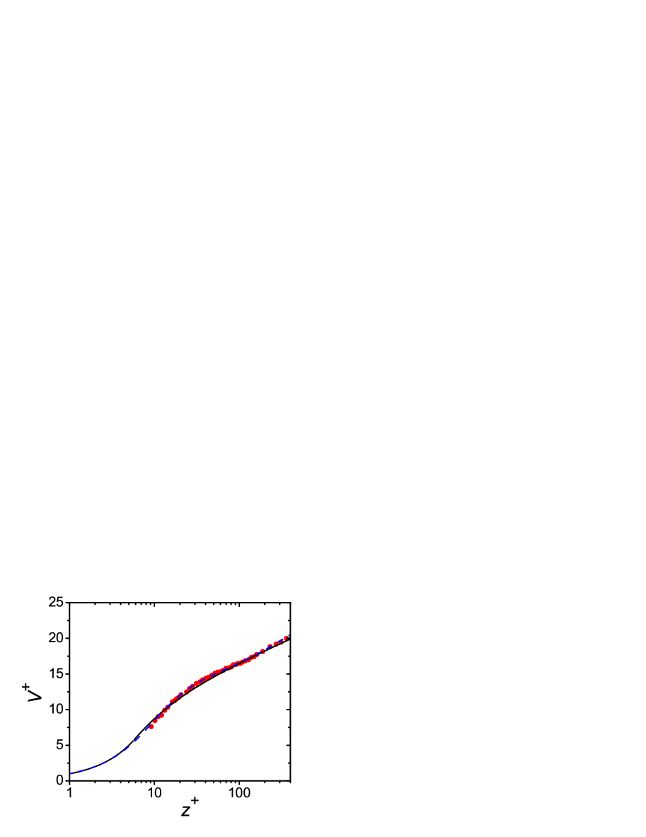
Figure 1: Mean velocity profiles $V^{+}(z^{+})$: black solid line – our analytical model, Eqs. (19) and (29); blue dashed line – results of the DNS simulation [3]; red points – experimental data [4].

In Fig. 2 we show analytical profiles of the Reynolds stress $W^{+}(z^{+})$, Eq. (28), in comparison with DNS. Due to the limited value of the friction Reynolds number in the DNS data [3], Re${}_{\lambda}=590$, we normalized the Reynolds stress using the local value of the momentum flux

$$\mathcal{P}(z^{+})=\mathcal{P}_{0}\Big{(}1-\frac{z^{+}}{\mbox{Re}_{\lambda}}\Big{)}\ .$$

The same normalization was used in Fig. 5 for the kinetic energy. Notice that the type of normalization [with $\mathcal{P}_{0}$ or $\mathcal{P}(z^{+})$] does not affect the mean profile (due to its slow, logarithmic dependence on $z^{+}$). Therefore, in the DNS data for mean velocity in Fig. 1 we used the simple normalization with $\mathcal{P}_{0}$. One can see in Fig. 2 an excellent agreement of our analytical results with the DNS results. The minor discrepancy is observed only in the viscous sublayer, $z^{+}\leq z^{+}_{\rm vs}$: in our simple approach the Reynolds stress and the turbulent kinetic energy are identically zero in this region, see Eq. (19). This stems from the disregard of the energy transfer term in the energy balance equation (7), which gives a non-zero level of turbulent activity close to the surface. As one sees however from Figs. 1 and 2, the account of the spacial transfer term does not lead to a considerable value of the Reynolds stress in the viscous sublayer and does not affect the mean velocity at all.

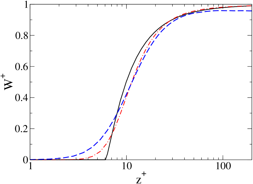
Figure 2: Profiles of the Reynolds stress $W^{+}(z^{+})$: black solid line – our analytical model, Eqs. (28) with $c^{2}_{\infty}=0.28$, red dash-dotted line – Eqs. (28) with function $c(z^{+})$, given by Eq. (31), and blue dashed line – results of the DNS simulation [3].

Another assumption that fails in the viscous and buffer layers is the approximation of constancy of the correlation coefficient $c^{2}_{\infty}\equiv W^{+}/K^{+}$. Note, however, that the expressions for the mean shear (27) and the Reynolds stress (28) remain valid even for $z^{+}$-dependent correlation coefficient $c_{\infty}\Rightarrow c(z^{+})$. In this case $z^{+}_{\rm vs}$ and $\kappa$ should be understood as $z^{+}$-dependent functions:

$$z^{+}_{\rm vs}\Rightarrow z^{+}_{\rm vs}(z^{+})\equiv\frac{a}{c(z^{+})}\,,\qquad\kappa\Rightarrow\kappa(z^{+})\equiv\frac{c^{3}(z^{+})}{b}\ .$$

In fact, we have chosen $c(z^{+})={\rm const}$ only to make possible an analytic expression for the mean velocity profile, Eq. (29). In our model we can easily account for the “realistic” $z^{+}$-dependence of the ratio $c^{2}$ integrating Eq. (27) numerically.

The actual dependence $c(z^{+})$, shown in Fig. 3 by blue dashed line, is taken from the public available statistical database, produced in Ref. [3] by DNS of the NSE for high-Reynolds turbulent flow in the channel geometry. One sees that $c(z^{+})$ decreases toward the surface. This fact can be understood by a series expansion for $W^{+}(z^{+})$ and $K^{+}(z^{+})$ for $z^{+}\to 0$ (see, e.g. [2]). This expansion shows that near the surface $W^{+}(z^{+})$ and $K^{+}(z^{+})$ behave as

$$W^{+}(z^{+})\sim({z^{+}})^{3}\,,\qquad K^{+}(z^{+})\sim({z^{+}})^{2}\,,$$

and therefore

$$c^{2}(z^{+})\sim z^{+}\,,\quad\mbox{near the surface.}$$ (30)

An origin of these dependencies is quite simple. At the surface, the rms values of the horizontal projections of the turbulent velocity $\sqrt{\langle{u_{x}^{+}}^{2}\rangle}$ and $\sqrt{\langle{u_{y}^{+}}^{2}\rangle}$ are zero according to the no-slip boundary conditions and grow with the height as $z^{+}$. This is not the case for the vertical projection, $\sqrt{\langle{u_{z}^{+}}^{2}\rangle}$. The incompressibility constraint dictates that

$$\frac{\partial u_{z}}{\partial z}=-\left(\frac{\partial u_{x}}{\partial x}+\frac{\partial u_{y}}{\partial y}\right)\propto z$$

and therefore the vertical projection increases only as $z^{2}$:

$$\sqrt{\left\langle{u_{x}^{+}}^{2}\right\rangle}\sim\sqrt{\langle{u_{y}^{+}}^{2}\rangle}\sim z^{+}\,,\quad\sqrt{\left\langle{u_{z}^{+}}^{2}\right\rangle}\sim({z^{+}})^{2}\ .$$

Accordingly,

$$W^{+}(z^{+})\equiv-\left\langle u^{+}_{x}\,u^{+}_{z}\right\rangle\sim\sqrt{\langle{u_{x}^{+}}^{2}\rangle\,\langle{u_{z}^{+}}^{2}\rangle}\sim({z^{+}})^{3}\,,$$

while the kinetic energy is dominated by the horizontal turbulent velocities,

$$K^{+}(z^{+})\simeq\frac{1}{2}\left[\langle{u_{x}^{+}}^{2}\rangle+\langle{u_{y}^{+}}^{2}\rangle\right]\sim({z^{+}})^{2}\,,$$

in agreement with Eq. (30).

To demonstrate how the actual dependence $c^{2}(z^{+})$ influence the mean velocity and turbulent activity profiles we suggest the following interpolation formula,

$$c^{2}(z^{+})=c^{2}_{\infty}\left[1-\exp\Big{(}-\frac{\ z^{+}}{z^{+}_{\rm cr}}\Big{)}\right]\,,$$ (31)

that has just two parameters, asymptotic value $c_{\infty}^{2}$ for $z^{+}\to\infty$ and the slope $c_{\infty}^{2}/z^{+}_{\rm cr}$ of the linear dependence (30) for $z^{+}\to 0$, near the surface. Dependence (31) with $c_{\infty}^{2}=0.28$ and $z^{+}_{\rm cr}=24$ is shown in Fig. 3 by red dash-dotted line. One sees that Eq. (31) closely fits the DNS data in the entire boundary layer and thus can be used as a realistic representation of the $W^{+}/K^{+}$ ratio in our model to find the analytical representation for the improved profiles of the Reynolds stress and kinetic energy, Eqs. (15, 28) and then, after numerical integration of Eq. (27) to get the improved mean velocity profile.

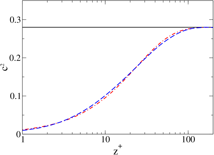
Figure 3: Blue dashed line – DNS data [3] for $c^{2}(z^{+})$, red dash-dotted line – suggested fit Eq. (31) for $c^{2}(z^{+})$, and horizontal black solid line – asymptotical value $c^{2}_{\infty}=0.28~{}\cite[cite]{[\@@bibref{}{DNS}{}{}]}$.

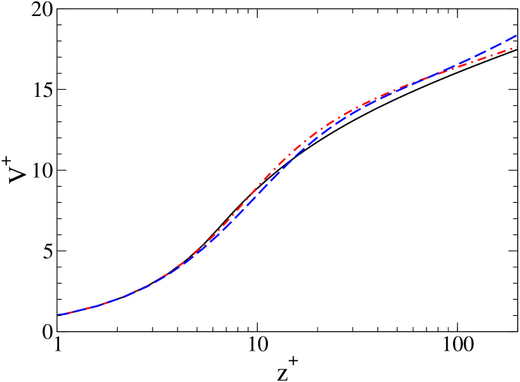
Figure 4: Mean velocity profiles $V^{+}(z^{+})$: black solid line – analytical profile, Eq. (29) with $a=3.2$, $b=0.27$ and $c=c_{\infty}$ (the same, as in Figs. 1-3) and red dash-dotted line – result of the numerical integration of Eq. (27) with fit function (31) for $c(z^{+})$ and $a=0.3$ and the same value of $b=0.27$. Blue dashed line – DNS data [3].

The comparison of the resulting profiles is given in Fig. 2 (Reynolds stress), Fig. 4 (mean velocity) and Fig 5 (kinetic energy). The profiles in the simple model with $c(z^{+})\Rightarrow c_{\infty}$ are denoted by black solid lines, the improved profiles with $z^{+}$-dependent coefficient $c(z^{+})$ – by red dash-dotted lines and the DNS profiles – by blue dashed lines. One sees in Fig. 4 that all mean velocity profiles nearly collapse: our approximation has no effect on the function $V^{+}(z^{+})$. For this object we prefer to take $c(z^{+})=c_{\infty}$ and to have a fully analytic model. The profile of the Reynolds stress, as one sees in Fig. 2, is improved in the viscous sublayer and is affected very little in the rest of boundary layer by account for $z^{+}$-dependence of $c(z^{+})$. As for the profile of the kinetic energy, Fig. 5, the neglect of the actual $z^{+}$-dependence of the coefficient $c(z^{+})$ leads to a significant underestimate of the kinetic energy in the buffer sublayer. In particular, the simple model does not exhibit a peak of $K^{+}(z^{+})$ in this region. If this peak is essential for some particular reasons, one should account for the actual $z^{+}$-dependence of $c(z^{+})$ at the expense of simplicity.

We have to stress, that the effect of the spacial energy transfer, neglected in our simple approach, is absolutely insignificant for the mean velocity profile (see Figs. 1 and 4). It has a minor importance for the profile of the Reynolds stress (Fig. 2) in the buffer layer and plays a more important role for the profile of kinetic energy, decreasing the amplitude of its peak and increasing the value of $K^{+}(z^{+})$ from the left of its maximum, in the viscous sublayer. Therefore, the necessity to account for the transfer term should be evaluated for each particular problem in hand.

In conclusion: In this paper we discussed in details a simple model of a turbulent flow over a flat plane that offer an analytical description of the mean velocity, Reynolds stress and kinetic energy profiles in the entire boundary layer. The calculated profiles exhibit an excellent agreement with the results of the laboratory experiments [4] and DNS [3] of the NSE. We discussed the effect of the approximations made in the analytical description of the profiles. We found a simple functional form for the experimental $z^{+}$-dependence of the correlation coefficient $c(z^{+})$, that allows to relax the approximation of the constancy of this coefficient. The profiles calculated with the help of this $z^{+}$-dependent coefficient $c(z^{+})$ account for all physically important features of all three profiles in the entire boundary layer region. The physical transparency and simplicity of the model allow its generalization for turbulently flowing suspensions, as it was demonstrated on the example of the problem of drag reduction by polymers in Refs. [1, 5, 6].

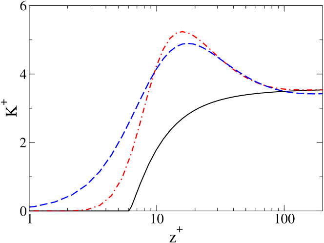
Figure 5: Mean profiles of the kinetic energy $K^{+}(z^{+})$: black solid line – analytical profile with $c=c_{\infty}$ red dash-dotted line accounts for the $z^{+}$-dependence (31) of $c$ and blue line – is the DNS profile [3].

- [1] L’vov, V.S., Pomyalov, A., Procaccia, I. and Tiberkevich, V: 2004, Drag Reduction by Polymers in Wall Bounded Turbulence, PRL, submitted, Also:nlin.CD/0307034
- [2] Pope, S. B.: 2000, Turbulent Flows, University Press, Cambridge.
- [3] Moser, R. G., Kim, J., and Mansour, N. N.: 1999, Direct numerical simulation of turbulent channel flow up to , Phys. Fluids 11, 943; DNS data at http://www.tam.uiuc.edu/Faculty/Moser/channel.
- [4] Zagarola, M. V. and Smits, A. J: 1997, Scaling of the Mean Velocity Profile for Turbulent Pipe Flow, Phys. Rev. Lett. 78, 239.
- [5] De Angelis, E., Casciola C., L’vov, V.S., Pomyalov, A., Procaccia, I. and Tiberkevich, V: 2004, Drag Reduction by a linear vicsosity profile, PRL, submitted, Also:nlin.CD/0401005.
- [6] Benzi, R., L’vov, V.S., Procaccia, I. and Tiberkevich, V: 2004, Drag Reduction by Polymers in Wall Bounded Turbulence, PRL, submitted, Also:nlin.CD/0402027