Periodically Varying Externally Imposed
Environmental Effects on Population Dynamics

Abstract

Effects of externally imposed periodic changes in the environment on population dynamics are studied with the help of a simple model. The environmental changes are represented by the temporal and spatial dependence of the competition terms in a standard equation of evolution. Possible applications of the analysis are on the one hand to bacteria in Petri dishes and on the other to rodents in the context of the spread of the Hantavirus epidemic. The analysis shows that spatio-temporal structures emerge, with interesting features which depend on the interplay of separately controllable aspects of the externally imposed environmental changes.

I  Introduction

The mathematical study of population dynamics has been a subject of great interest in recent years, with application widely spread among different fields. An example is the description of emerging patterns in bacterial colonies jaco ; waki ; lin ; nels ; lito ; thesis ; kk . Other studies describe the behavior of the populations of superior organisms such as insects and rodents chule ; ale ; oku ; murr .

If, in basic models for the description of the evolution of a given population, we focus attention on reproduction, competition for resources, and diffusion, the Fisher equation fish ; murr appears to be a useful mathematical tool:

$$\frac{\partial u\left(x,t\right)}{\partial t}=D\frac{\partial^{2}u\left(x,t\right)}{\partial x^{2}}+au\left(x,t\right)-bu^{2}\left(x,t\right).$$ (1)

Diffusion with coefficient $D$ is considered here as well as the growth of the population at rate $a$ and a competition process weighted by $b$, also containing environmental features. In the present paper, we consider effects of spatio-temporal dynamics in the nonlinear term as a representation of externally imposed or seasonal environmental variations. We thus take $b$ in Eq. 1 to be space and time dependent, $b(x,t)$. Environmental variations could alternatively be considered as affecting $a$ (such that $a$ is dependent on time and space rather than $b$) as has been done in some earlier studies lin ; kk . However, we restrict our attention to a constant $a$ and varying $b(x,t)$ because this allows us to define a Fisher velocity and size in terms of a constant $a$. Following kk we consider a bounded region which will be referred to as a $bubble$ of favorable conditions suitable for the survival of a given species. Outside of this region the environmental conditions are so harsh that there is no possibility of survival.

Associated with the Fisher equation fish there is a natural velocity and a natural length, $2\sqrt{Da}$ and $\pi\sqrt{D/a}$, respectively. The former is known as the Fisher velocity and is the velocity at which fronts tend to travel after adjustments from most initial conditions murr . Thus, an arbitrary shape of the initial population with compact support will have fronts that move, after initial transients, with the Fisher velocity. It is an important quantity in experiments on bacteria with moving masks lin as it represents the minimum mask velocity at which bacteria tend to extinction, rather than being able to follow the bubble through the combined effect of growth and diffusion. The Fisher length $\pi\sqrt{D/a}$ arises kk ; skellam in the bacterial context as the minimum length of the mask below which the steady state population of the bacteria vanishes as the bacteria diffuse out of the masked area quicker than they can grow to any finite saturation value. The Fisher length is thus the ‘diffusion length’ within the growth time (reciprocal of the growth rate $a$).

Consideration of these two quantities suggests that it is natural to envisage two observations involving externally imposed periodic variation of the environment. The first is one in which experiments of the kind reported in ref. lin are carried out with the velocity varying periodically, in other words with the bubble repeatedly returning to its original position. This is the oscillating bubble case. The second experiment is one in which the bubble extent is made to vary from a large size to one below the Fisher length (i.e. the extinction size). The objective of the latter ($breathing$ bubble) experiment is to analyze extinction tendencies under periodic variations of the bubble size. We analyze these two hypothetical experiments in this paper through numerical calculations based on a Crank-Nicholson scheme.

II Traveling bubble

Solutions of the Fisher equation for bounded domains, corresponding to static bubbles, have been already discussed in kk and references therein. A natural change, to be considered as a first approximation to the problem addressed here, is to allow a translation in the bubble. We have performed a brief analysis of situations where the velocity is constant and the system’s behavior corresponds to that of a moving front, as well as others where the velocity of the bubble changes continuously. For the former case, and as mentioned in murr , we recover a critical velocity beyond which the front will no longer survive, see bold curve of 1. As $b\rightarrow\infty$ at the boundaries of the bubble, the curves will abruptly go to zero, rather than asymptotically as above. The analysis of this situation can be done by making a change of variables on Eq. (1). If we set $\xi=x-ct$ we obtain the following equation which is valid in the moving frame accompanying the bubble.

$$D\frac{\partial^{2}u\left(\xi\right)}{\partial\xi^{2}}+au\left(\xi\right)-bu^{2}\left(\xi\right)+c\frac{\partial u\left(\xi\right)}{\partial\xi}=0.$$ (2)

By measuring the maximum population density, $u_{max}$, of the front solution or the steady solution in a moving frame, we obtain a curve that will be useful in interpreting the following results. As the bubble accelerates in the moving frame, the system is not allowed to relax into a steady state, see the accelerating curve of Fig.1. The time involved in the changes induced by the acceleration of the bubble compete with the relaxation time of the system. We will leave these results for now and recall them later to understand the following analysis.

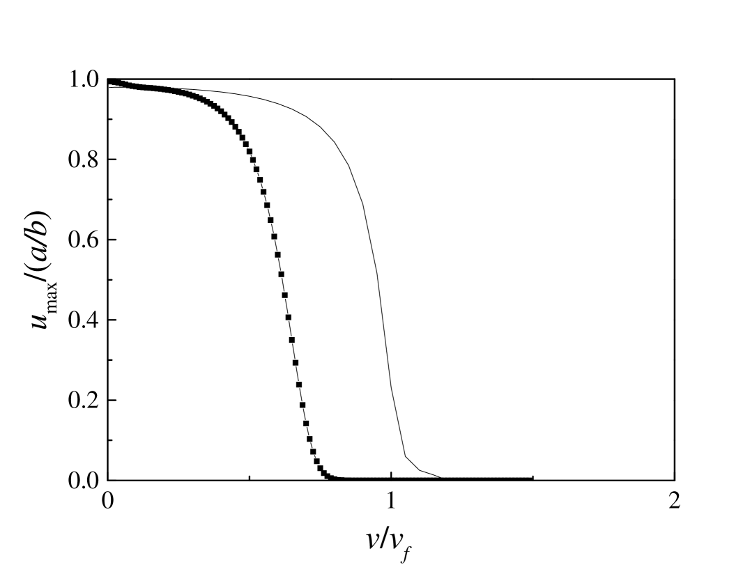
Figure 1: The bold curve depicts $u_{max}$ as the bubble moves adiabatically; acceleration is affectively zero. The remaining curve displays $u_{max}$ for a bubble accelerating linearly at $.1a^{2}W_{c}$.

III Oscillating Bubble

Here, the habitable bubble of fixed width oscillates as a whole. We study two cases: sinusoidal velocity, and a velocity which is constant but suddenly changes direction at a given distance away from the original position. All points within the amplitude of oscillation will thus be covered periodically for varying amounts of time. For the purpose of comparison, we will consider the velocity to be an average velocity for the sinusoidal case. The parameters involved are the average velocity of the bubble, $v$, the amplitude of oscillation characterized by the distance between the center of the bubble at the turning points, $A$, the length of the bubble, $W$, and the Fisher parameters: the diffusion coefficient, $D$, the growth rate, $a$, and the competition term, $b(x,t)$. For the following analysis, $b(x,t)$ is a step function that defines the shape of the bubble. We have examined the following aspects of Eq. (1):

• The role of each of the three parameters, $v$, $A$, and $W$, in the dynamics of the population.

• How the two cases (sinusoidal velocity and constant velocity) differ from each other.

• Qualitative characteristics and comparisons between solutions for various parameter sets.

• The evolution of the population as diffusion goes to zero.

• The appearance of a curious dipping phenomenon.

III.1 Numerical Results for D>0

It is helpful to divide the behavior into two regimes which correspond to no-extinction and extinction. The parameters $A$, $W$, and the critical bubble width, $W_{c}=\pi\sqrt{(}D/a)$ kk ; skellam , are sufficient to define these regimes. In the steady state, bubble widths smaller than the critical value are unable to support a population density. This feature now manifests itself in the amount of overlap between the two extremes of an oscillating bubble. For $A<W$ there will be an area that is permanently covered by the bubble. When this covered area, from now on referred to as the $overlap$, is greater than the critical width, the population will always survive to some degree. This regime is bounded by $0<A<(W-W_{c})$.

In the other regime, extinction may occur when there is an overlap that is less than the critical value, $(W-W_{c})<A$. The distance between the inner edges of the bubble when $A>W$ will be called the $separation$, $(A-W)$. Naturally, when there is a separation, no single location will receive continuous coverage by the bubble.

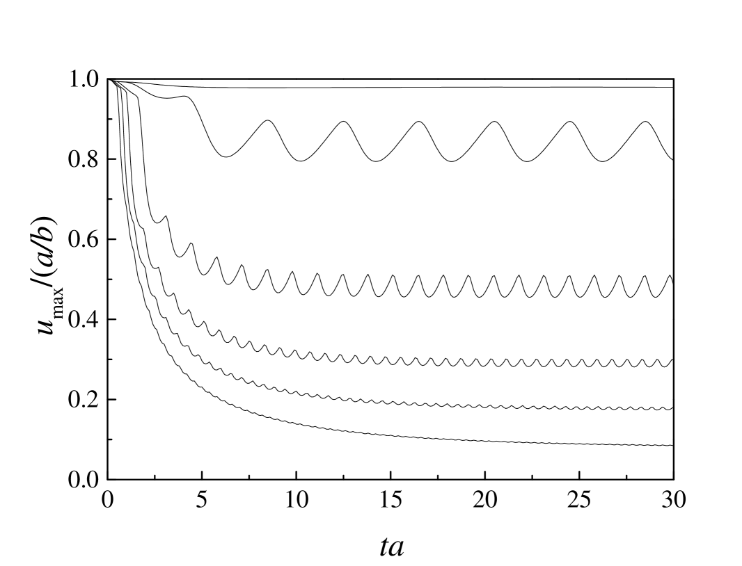
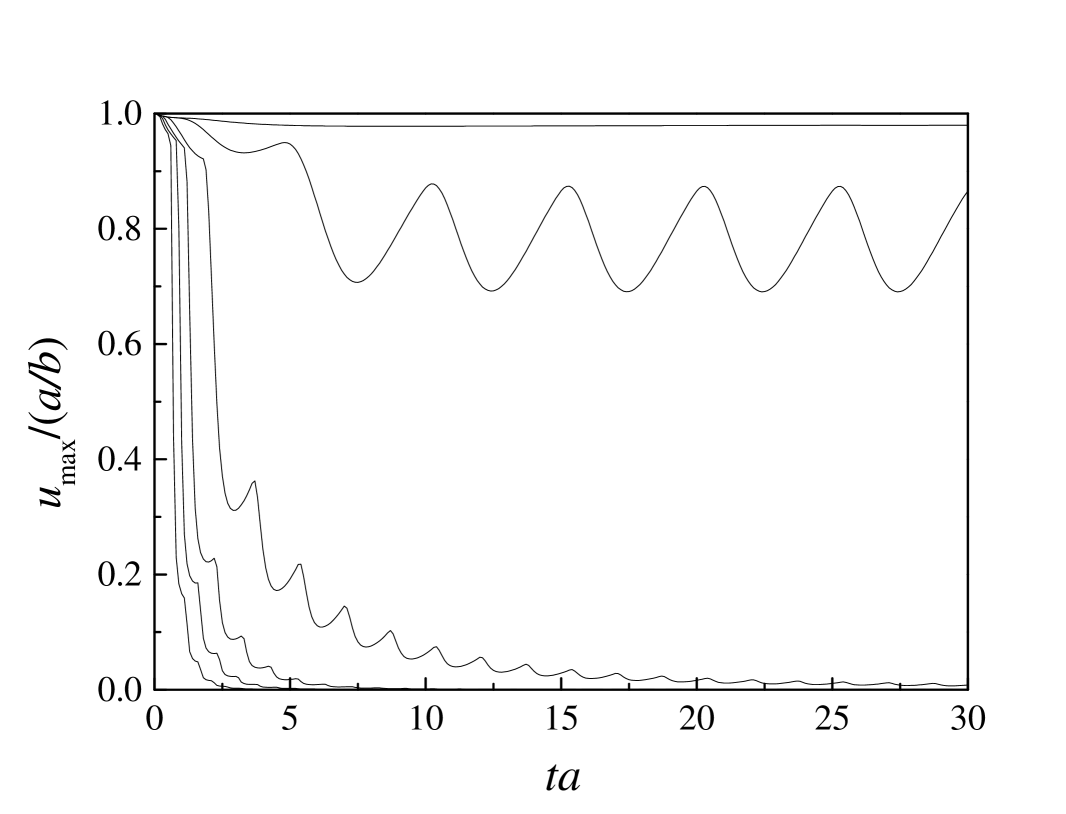
Figure 2: Temporal evolution of $u_{max}$ where in (a) $A=8W_{c}$, (b) $A=10W_{c}$, and $W=10W_{c}$ in both. Each curve is characterized by one of seven sinusoidal bubble velocities, $.1aW_{c}$, $1aW_{c}$, $3aW_{c}$, $5aW_{c}$, $7aW_{c}$, and $10aW_{c}$ where $v_{f}=aW_{c}$ when $D=aW_{c}^{2}$, as in the plots above. Higher velocities induce lower maximum population density values and thus drive a population closer to extinction as the amplitude of oscillation increases.

For either regime, if the velocity is below the Fisher velocity, $v_{f}$, the population will be able to follow the oscillating bubble. As the velocity increases it becomes more difficult for the population density to keep up with the moving bubble (via diffusion and new growth). Some of the population falls prey to the harsh environment which quickly reduces the density. If $b(x,t)$ is infinite for |x|>W/2, the exposed population will go extinct, never to return. For realistic as well as numerical purposes, we will consider $b$ outside the bubble to be a large but finite number. Once outside of the bubble, the population decreases immensely yet it now retains the ability to regenerate. Due to the extended amount of time that either end of the bubble’s trajectory is sheltered, peaks of increased population density form at these extremes. As the velocity is increased, these peaks become more pronounced with respect to the maximum population density in the center of the bubble’s trajectory. They also come more frequently since the bubble traverses the same period of oscillation more often, see in Fig. 2 and Fig. 3. The entire density profile oscillates spatio-temporally as the velocity increases and varies with the amount of overlap or separation.

For the zero extinction regime, high velocities effectively wash out the oscillatory behavior and the peaks merge so that the length of permanent overlap then determines the population density. The behavior of the population in the extinction regime, $(W-W_{c})<A$, is the same except for one crucial characteristic. Again, the peaks at the endpoints come closer together for higher velocities, but they never merge. The population dies out before a constant density forms in the center. As $A$ increases, extinction occurs for smaller and smaller velocities.

In the discussion above an $average$ velocity of the bubble was assumed. We now make a distinction between two types of velocities and their relative affects on the population density. A bubble moving with sinusoidal velocity lingers for longer time over the end points of its trajectory and for shorter time in the center as compared to the constant velocity bubble. For a single location, a larger population density is permitted to grow if more time is spent under the bubble. The basic qualitative differences of the population density thus follow from these two aspects. Though the two velocities produce the same essential behavior, we find that there indeed exists a difference between the two after long times. This will be addressed in the final section.

To further understand the structural changes of the population, we have examined the maximum population density as it oscillates parametrically in time. The shape that is outlined can be roughly characterized by a $bowtie$, Fig. 3. The densities of the maxima, minima, center, and the spatial extremes are the four features that comprise the qualitative differences between bowtie morphologies.

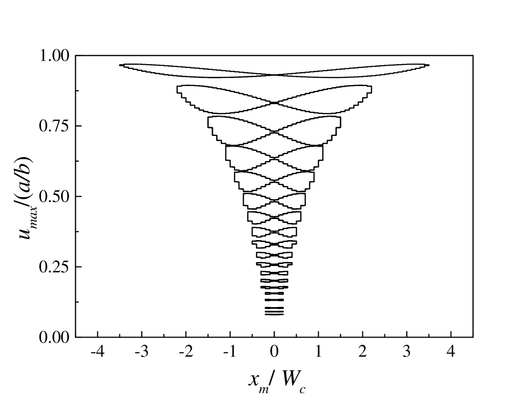
Figure 3: A variety of bowties exhibit the affects for different values of $v$ when a bubble of $A=8W_{c}$, $W=10W_{c}$ and $D=aW_{c}^{2}$ moves with sinusoidal velocity. Velocities from top to bottom range from $aW_{c}$ to $10aW_{c}$ and increment by $.5aW_{c}$ where $v_{f}=aW_{c}$ when $D=aW_{c}^{2}$. The trajectories are parametric in time such that $u_{max}$ is increasing at the endpoints.

As the average velocity increases these four points of comparison within the bowtie undergo changes in proportion. The maxima of the bowtie move closer to the center (recall that in the no-extinction regime these maxima eventually merge). The minima move farther from the center. The spatial spread of the bowtie is smaller and the overall values of the population density decrease for all positions. The difference between the maxima and minima of the bowtie, $A_{b}$ (the amplitude of oscillation of the maximum population density) initially increases and then decreases as velocity increases. Fig. 4 depicts the abrupt appearance and then gradual decay of the bowtie as a function of velocity. The bowtie appears in both nondiffusive systems and diffusive systems. Bowties of the former develop amplitudes larger than those of the latter. Also, bowties are formed at lower velocities for the nondiffusive than for the diffusive system.

III.2 Analytic Results for D=0

We begin by considering the Fisher equation where the oscillation of the bubble is explicitly built into the argument of the competition parameter $b(x,t)$ of Eq.(1).

$$\frac{\partial u(z,t)}{\partial t}=a\,u(z,t)-b(z+\int_{0}^{t}v(s)\,ds)\,u(z,t)^{2}+D\,\frac{\partial^{2}u(z,t)}{\partial z^{2}}$$

The transformation $\phi=1/u$ yields an equation of the form

$$\frac{\partial\phi(z,t)}{\partial t}+a\,\phi(z,t) =$$ (3)

$$b\left(z+\int_{0}^{t}v(s)\,ds\right)+D\left[\frac{\partial^{2}\phi(z,t)}{\partial z^{2}}-\frac{2}{\phi}\left(\frac{\partial\phi}{\partial z}\right)^{2}\right].$$

By allowing $D=0$, we recover the equation for a highly damped linear oscillator that is driven by an external force proportional to $b(z+\int_{0}^{t}v(s)\,ds)$. The population will thus follow the periodic forcing function with a lag. This oscillator interpretation clarifies the structure of the bowtie. Each location grows periodically, with a temporal lag, at the behest of the driving term. The locations at the edges of the bubble’s spatial trajectory will have higher population densities because the driving oscillator lingers for longer time at a lower value (less harsh conditions).

An additional transformation

$$x=z+\int_{0}^{t}v(s)\,ds,$$

and letting $D=0$ leads to,

$$\frac{\partial\phi(x,t)}{\partial t}+v(t)\,\frac{\partial\phi(x,t)}{\partial x}+a\,\phi(x,t)=b(x).$$ (4)

The solution, as derived in luca , was found to be,

$$\phi(x,t) = e^{-a\,t}\,\phi_{0}\,(x-\int_{0}^{t}v(s)\,ds)$$ (5)

$$+\int_{0}^{t}e^{-a\,(t-t^{\prime})}\,b\left(x-\int_{0}^{t^{\prime}}v(s)\,ds\right)\,dt^{\prime}$$

and finally, $u(x,t)$ explicitly as

$$u(x,t) =$$

$$\frac{u_{0}(x-\int_{0}^{t}v(s)\,ds)}{e^{-a\,t}+u_{0}(x-\int_{0}^{t}v(s)\,ds)\,\int_{0}^{t}e^{-a\,(t-t^{\prime})}\,b(x-\int_{0}^{t^{\prime}}v(s)\,ds)\,dt^{\prime}}.$$

As the bubble’s velocity greatly surpasses the Fisher velocity, the effect of diffusion becomes negligible. The diffusion length per time competes with the velocity of the bubble. Diffusion is thus limited by the time a single location is covered by the bubble and has little effect when velocity is high. A solution thus exists in the high velocity limit, refer to Fig. 4.

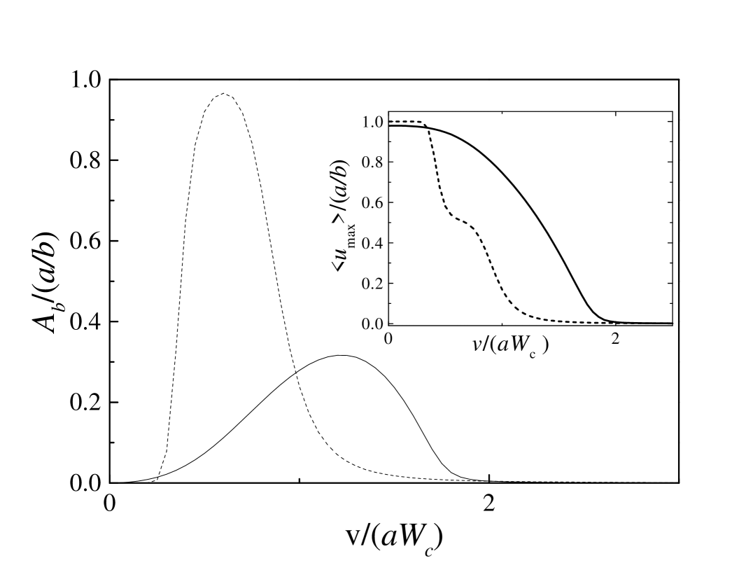
Figure 4: The amplitude of the bowtie is plotted against the average velocity (which here varies sinusoidally). The inset shows the average $u_{max}$ after long time. The combination of the both show the validity of the analytic solution in the high velocity regime when the curves for $D=aW_{c}^{2}$ and $D=0$ converge.

When the velocity is relatively low, $v<v_{f}$, population migration occurs via diffusion and new growth. By letting $D\rightarrow 0$ (correspondingly, $v_{f}\rightarrow 0$ and critical overlap$\rightarrow 0$) one might conclude that a population cannot maintain itself unless there is a bit of overlap. This is true when the velocity is such that growth cannot occur within the short period of coverage by the bubble. However, when these two rates (bubble velocity and $aW$) are comparable, oscillations in the population density again arise in the diffusionless case. The bowties in these circumstances vaguely resemble those of before. When $A<W$ the maximum population density is always saturated; there are no means by which to leave a sheltered region without diffusion. When $A>W$, the bowtie limits to a $U$ shape.

IV Breathing bubble

The breathing bubble corresponds to a situation when the width of a anchored bubble varies in time. As before, we consider several cases and for each of them a family of values for the involved parameters. These parameters are the velocity of the variation of the width, the mean width of the bubble, the amplitude of the breath, and again, the Fisher parameters of Eq. (1). We are interested in analyzing the relationship between the existence of critical values and the response of the population density to a changing environment. We first take the case when the bubble width oscillates at a constant speed but always preserves a size above the critical one. The interesting aspect of this situation occurs at the boundaries of the bubble where population fronts are formed. The fronts can follow the movement of the bubble when the velocity of the breathing motion is under a critical value. Above this critical value, the population is confined to the minimum size of the bubble, which indicates that the population front can no longer follow the changes of the bubble. To show this we display in Fig. 5 the relative amplitude of the oscillation of the population front, $A_{f}/A$ vs. the speed of the bubble breath, where $A$ is the amplitude of breathing.

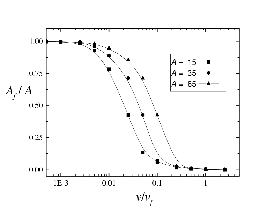
Figure 5: Amplitude of the front oscillations for several velocities of the bubble where $D=aW_{c}^{2}$.

We observe that at a critical value this amplitude goes to zero. That is, in spite of the changing size of the bubble, the population density remains bounded statically.

Instead of a constant value for the velocity of breathing, we can take a fixed frequency for a sinusoidal behavior. The frequency is associated with the breathing motion of the bubble boundaries. The results are analogous to those displayed in Fig. 5.

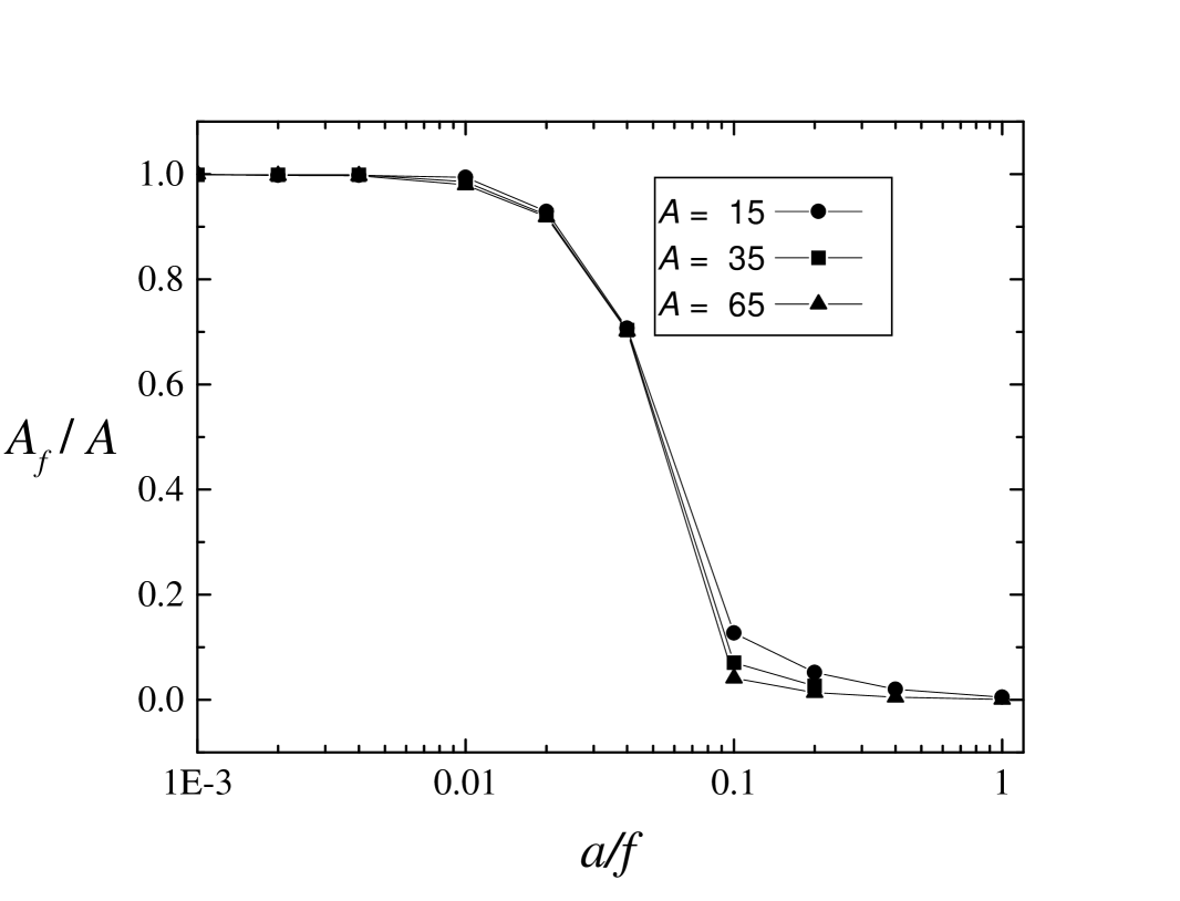
Figure 6: Amplitude of the front oscillations for several values of the inverse of the frequency of breathing of the bubble where $D=aW_{c}^{2}$.

No qualitative differences were found.

When the minimum size attained by the bubble during the breathing is under the critical size, the situation is different. It is not enough to plot, as in previous examples, the amplitude of the oscillation of the front because some variations in the maximum density of the population are also observed. To visually understand what is happening we again plot the temporal behaviour of maximum value of the population, $u_{max}$ as a function of the momentary width of the breathing bubble. This is what is shown in Fig. 7, where the trajectories are traversed clockwise.

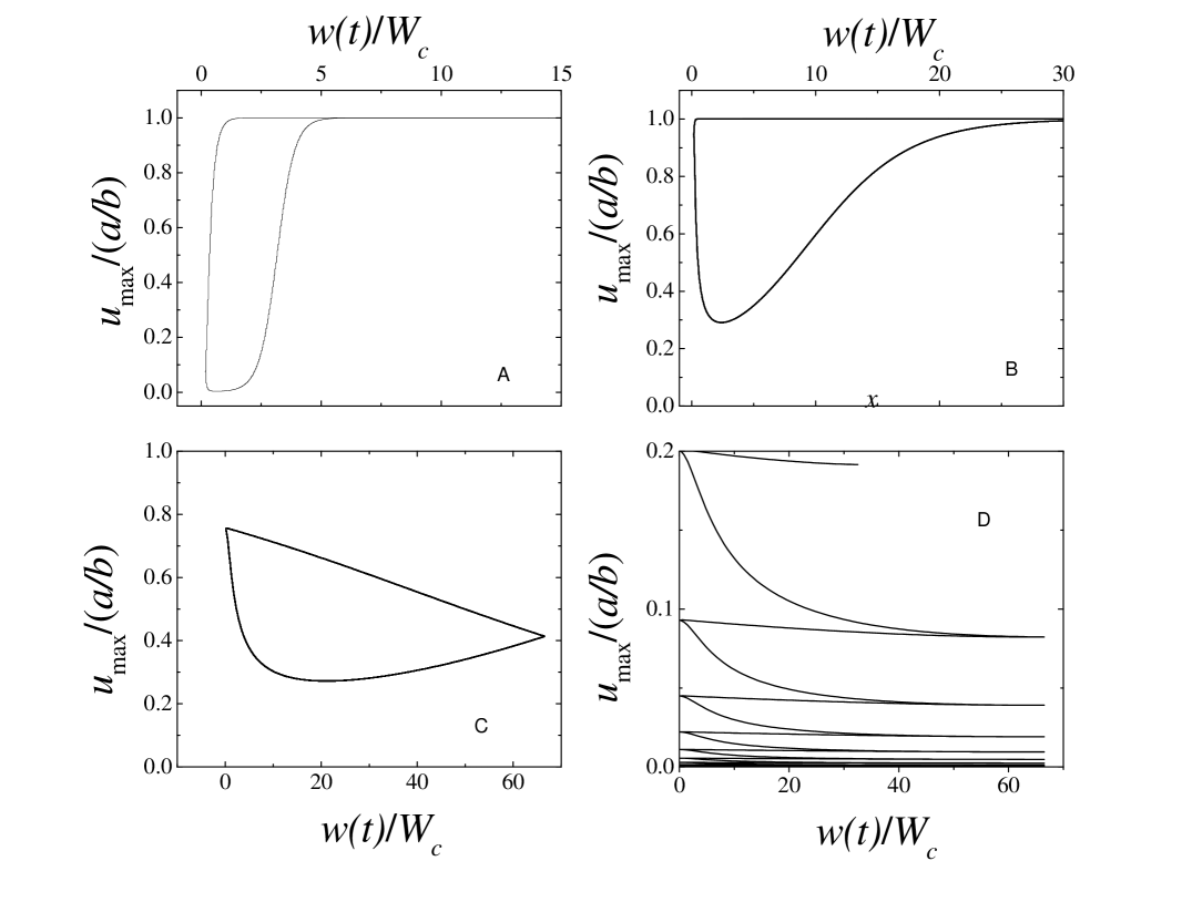
Figure 7: Maximum value adopted by the population as a function of the instantaneous width of the bubble. The velocity of breathing is: a)0.1$aW_{c}$ b)1$aW_{c}$ c)10$aW_{c}$ d)40$aW_{c}$, and $D=aW_{c}^{2}$.

As observed in the plots, if the velocity is low enough, the size of the bubble will be under the critical size long enough to provoke the extinction of the population. On the contrary, for higher values of the velocity there is a range of values at which the population can survive. The response of the population to changes is much slower than the dynamics of the environment. Each of the results obtained in this case are essentially the same as the corresponding results from the oscillating bubble. In particular, the results displayed in Figs. 5 and 6 can be associated with the discussion included in the previous section, those included in Fig. 7 are analogous to the bowtie effect.

V Further features

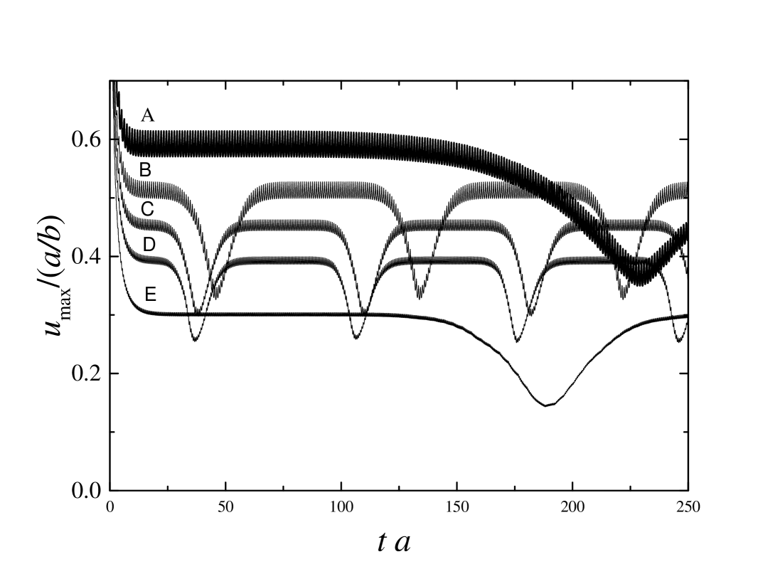
Figure 8: After long times a periodic dip in all values of $u_{m}ax$ is observed for constant velocities. The sampling above, (A, B, C, D, and E) corresponds to velocities (3.5$aW$, 4.5$aW$, 5.5$aW$, 6.5$aW$, and 8.5$aW$, respectively) where $v_{f}=aW$ because $D=aW_{c}^{2}$.

We now return to a surprising feature that arises only in the presence of constant bubble velocity and diffusion. Probing longer times reveals an overlying oscillation in the population density profile. For diffusive systems, $D>0$, and constant velocities, the entire bowtie dips down and then back up again in a periodic manner with constant amplitude. For different velocities the bowtie dips and rises with different periods and amplitudes, see Fig. 8. Also, notice that as velocity increases, the frequency of the alternative dip doesn’t simply increase as well. Nor does the amplitude of the dip appear to change with the velocity. Sinusoidal velocities do not produce this affect. Further analysis is necessary to completely understand the origin of this behavior and its relation to the two required conditions, diffusion and constant bubble velocity.

VI Conclusions

In the present work, we have numerically studied the behavior of a population whose dynamics are described by a modified Fisher equation with additional environmental variations. Analytic solutions were also considered for simplified examples. The results presented here show that besides the expected behavior some surprising features arise. There exist two main parameters that characterize the evolution of a given population: the Fisher length and Fisher velocity. A given group of individuals will not survive if the habitat size is smaller than the Fisher length. At the same time, the population will not be able to maintain saturation when the habitat moves with a velocity higher than the Fisher velocity. With these two considerations we have examined two types of periodically varying environments. Though extinction of the population was verified in conditions corresponding to the two situations mentioned above, it was also found that some nontrivial scenarios can also arise. Situations in which extinction was expected exhibited what we called the bowtie effect. An interplay between the time associated to the transient towards extinction and the periods of the changing environments is the cause of unexpected behavior of the population. We have also verified that there is a correspondence between the results obtained when considering oscillatory or breathing bubbles, though the situations are different. A diffusionless approximation helped to understand the origin of the observed phenomena in terms of oscillating perturbations. Perhaps the most unexpected result is that depicted in Fig.8. An explanation for these features is still in progress.

VII Acknowledgements

This work is supported in part by the Los Alamos National Laboratory via a grant made to the University of New Mexico (Consortium of the Americas for Interdisciplinary Science), by the NSF’s Division of Materials Research via grant No DMR0097204, by the NSF’s International Division via grant No INT-0336343, and by DARPA-N00014-03-1-0900.

References

- (1) E. Ben-Jacob, I. Cohen and H. Levine. Adv. Phys. 49 ,395-554 (2000)
- (2) J. Wakita, K. Komatsu, A. Nakahara, T Matsuyama, M. Matsushita. Journ. Phys. Soc. Japan 63, 1205 (1994).
- (3) A. L. Lin, Bernward A. Mann, Gelsy Torres-Oviedo, Bryan Lincoln, Josef Kas, Harry L. Swinney, "Localization and extinction of bacterial populations under inhomogeneous growth conditions", Biophys. J. (in press). Preprint q-bio.PE/0310032.
- (4) D.R. Nelson and N.M. Shnerb, Phys. Rev. E 58,1383 (1998); K.A. Dahmen, D.R. Nelson and N.M. Shnerb, J. Math Biology, 41,1 (2000).
- (5) M. Fuentes, M. N. Kuperman, V. M. Kenkre Phys. Rev. Lett. 91, 158104 (1-4) (2003)
- (6) A. M. Delprato, A. Samadani, A. Kudrolli, L. S. Tsimring, Phys. Rev. Lett., 87, 158102 (2001).
- (7) V. M. Kenkre, M. N. Kuperman Phys. 67 051921 (1-5) (2003).
- (8) G. Abramson, V.M. Kenkre Phys. 66, 011912 (1-5) (2002).
- (9) M.A. Aguirre, G. Abramson, A.R. Bishop, V.M. Kenkre Phys. 66, 041908 (1-5) (2002).
- (10) A. Okubo and S. Levin. Diffusion and Ecological Problems. Second Edition, Springer. (2001).
- (11) J. Murray. Mathematical Biology. Second Edition, Springer. (1993).
- (12) R.A.Fisher, Ann. Eugen. London 7, 355-369 (1937).
- (13) J. C. Skellam. Biometrika. 38, 196 (1951).
- (14) L. Giuggioli, V. M. Kenkre, Physica D, 183245-259 (2003).
- (15) C. T. Lee, M. F. Hoopes, J. Diehl, W. Gilliland, G. Huxel, V. Leaver, K. McCann, J. Umbanhowar and A. Mogilner, J. Theor. Biol. 201
- (16) A. Mogilner, L. Edelstein-Keshet, J. Math. Biol. 38, 534 (1999).
- (17) V. M. Kenkre, in Patterns, Noise, and the Interplay of Nonlinearity and Complexity, eds. V. M. Kenkre and K. Lindenberg, Proceedings of the PASI on Modern Challenges in Statistical Mechanics, AIP (2003), scheduled for publication.
- (18) C. Tsallis, J.Stat. Phys. 52, 449 (1988).
- (19) G. Abramson, A. Bishop and V. M. Kenkre, Physica A, 305