Controlling spatiotemporal chaos
in oscillatory reaction-diffusion systems
by time-delay autosynchronization

Abstract

Diffusion-induced turbulence in spatially extended oscillatory media near a supercritical Hopf bifurcation can be controlled by applying global time-delay autosynchronization. We consider the complex Ginzburg-Landau equation in the Benjamin-Feir unstable regime and analytically investigate the stability of uniform oscillations depending on the feedback parameters. We show that a noninvasive stabilization of uniform oscillations is not possible in this type of systems. The synchronization diagram in the plane spanned by the feedback parameters is derived. Numerical simulations confirm the analytical results and give additional information on the spatiotemporal dynamics of the system close to complete synchronization.

, ,

1 Introduction

Pattern formation in spatially extended systems far from thermal equilibrium has attracted much attention in recent years and became a field of active research [1, 2]. A large class of these systems is described by equations of the reaction-diffusion type. In such systems, a broad variety of complex spatiotemporal patterns has been observed, ranging from travelling pulses and target patterns to rotating spiral waves and spatiotemporal chaos. Important examples are chemical reaction-diffusion systems such as the Belousov-Zhabotinsky reaction or catalytic surface chemical reactions [3, 4, 5], as well as semiconductor and biological systems [6, 7].

Many systems show oscillatory dynamics of their individual elements. Close to the onset of oscillations, the equations describing any oscillatory system can be reduced to a simple universal equation for the complex oscillation amplitude, the complex Ginzburg-Landau equation (CGLE) [8, 9]. For a distributed system with diffusive coupling, the CGLE corresponds to the normal form of a supercritical Hopf bifurcation. Although the CGLE is strictly valid only in the immediate vicinity of the oscillation onset, it has been found in many cases that its qualitative predictions also hold within a wider range near the bifurcation point. The CGLE thus provides a general framework for studying common features of the dynamical behaviour in oscillatory reaction-diffusion systems. If oscillations are synchronized, uniform oscillations can be established in the medium or regular spatiotemporal patterns can emerge.

If the Benjamin-Feir criterion is met, synchronous oscillations become unstable and a turbulent state develops where two types of chaotic behaviour can be distinguished. In the state of phase turbulence, the local oscillation phase exhibits weak irregular fluctuations while the real amplitude remains saturated showing only small variations [8]. Amplitude or defect turbulence is characterized by strong fluctuations of both phase and amplitude which are due to the presence of defects, the locations with a vanishing amplitude [10].

Over the past decade, problems of chaos control became to play a central role in the studies of chaotic dynamics [11]. Inspired by the pioneering work of Ott, Grebogi, and Yorke (OGY) [12], control of chaos has been studied in the context of many different dynamical systems [13, 14, 15] However, the OGY method is designed to control chaos in low-dimensional dynamical systems. It requires continuous extensive analysis of the system dynamics which is virtually impossible to carry out in the case of fully developed high-dimensional turbulence in spatially extended systems. A different empirical control method based on implementing a delayed feedback loop was proposed by Pyragas and is known as time-delay autosynchronization (TDAS) [16, 17]. In this method, a feedback signal $F$ is applied to the system that is proportional to the difference between the delayed value of a given system variable $u$ and its instantaneous value, $F\sim u(t-\tau)-u(t)$. This approach is easily extended to spatially distributed experimental systems that often do not allow individual addressing of their local elements. Then, the global feedback signal is generated from the integral value of $u$ over all system elements. In recent studies, the TDAS method has been used in a number of different dynamical systems [18, 19, 20] and was modified and improved considerably [21, 22, 23]. For the CGLE, the action of local TDAS has been previously considered [24, 25].

The present work was motivated by our experimental study of catalytic CO oxidation under TDAS [26]. The catalytic CO oxidation on a platinum (110) single crystal surface constitutes the most thoroughly studied example among a class of simple heterogeneous catalytic reactions for which reaction-induced spatiotemporal pattern formation has been reported [5]. It displays a particularly rich variety of spatiotemporal concentration patterns [27] that can be modeled numerically using a simple model of three coupled partial differential equations [28, 29]. The effect of global delayed feedback on pattern formation in catalytic CO oxidation was studied previously using a different time-delay feedback scheme [30, 31, 32]. The same feedback scheme was also investigated in detail in the context of the complex Ginzburg-Landau equation [33, 34]. Our work on suppression of chemical turbulence in catalytic CO oxidation using the TDAS scheme [26] was focused on investigating the question of invasiveness. We found in the experiment that, although we could reduce the magnitude of the feedback signal considerably, we were not able to reach the ideal limit of a vanishing feedback signal in the state of control. In the present work, we use the complex Ginzburg-Landau equation as a general model for spatially extended oscillatory systems to study common aspects of control of diffusion-induced chemical turbulence by TDAS.

The paper is organized as follows. In the next section, the physical problem and the corresponding equations will be introduced. In Section 3, we analyze the stability of uniform oscillations in the presence of TDAS and derive a synchronization diagram. Numerical simulations of the complex Ginzburg-Landau equation with TDAS are described in Section 4. The paper ends with conclusions and a discussion of the obtained results.

2 Formulation of the problem

In absence of feedback, the dynamics of a chemical reaction-diffusion system can be generally described by a set of coupled partial differential equations

$$\mathbf{\dot{u}}=\mathbf{f}(\mathbf{u}\,,\mathbf{p})+\mathbf{D}\nabla^{2}\,\mathbf{u}\,,$$ (1)

where $\mathbf{u}=(u_{1},u_{2},...,u_{N})$ represents concentrations of reacting species and $\mathbf{D}$ is their diffusion matrix. The set of nonlinear functions $\mathbf{f}(\mathbf{u},\mathbf{p})$ of the concentrations $\mathbf{u}$ accounts for the reaction part of the dynamics and depends on a number of parameters $\mathbf{p}=(p_{1},p_{2},...,p_{M})$, such as rate constants and external conditions.

Suppose that the dynamics of system (1) is such that a supercritical Hopf bifurcation occurs when crossing a certain threshold $\mathbf{p}=\mathbf{p}_{0}$ in the parameter space. Close to the onset of oscillations, system (1) can be transformed to a simple description of the dynamics in terms of a complex oscillation amplitude $\eta(x,t)$. This transformation is based on retaining only the leading critical modes that govern the dynamics close to the bifurcation point. It yields as equation of motion for the amplitude $\eta(x,t)$, the complex Ginzburg-Landau equation [8],

$$\dot{\eta}=(1-\mbox{i}\omega)\eta-(1+\mbox{i}\beta)|\eta|^{2}\eta+(1+\mbox{i}\varepsilon)\nabla^{2}\eta\,,$$ (2)

where the parameters $\omega$, $\beta$, and $\varepsilon$ denote the linear oscillation frequency, the nonlinear frequency shift, and the linear dispersion coefficient, respectively. When the condition $1+\varepsilon\beta<0$ of the Benjamin-Feir instability is satisfied, uniform oscillations are unstable and turbulence spontaneously develops in the system. To control the turbulence, global feedback can be introduced. In the presence of global time-delayed feedback, the considered system is described by the equation

$$\dot{\eta}=(1-\mbox{i}\omega)\eta-(1+\mbox{i}\beta)|\eta|^{2}\eta+(1+\mbox{i}\varepsilon)\nabla^{2}\eta+F(t)\,,$$ (3)

where the feedback term is given by

$$F(t)=\mu\,\mbox{e}^{\mbox{\scriptsize i}\chi}(\bar{\eta}(t-\tau)-\bar{\eta}(t))\,,$$ (4)

and

$$\bar{\eta}(t)=\frac{1}{L}\int_{0}^{L}\eta(x,t)\mbox{d}x\,.$$ (5)

Here, $\mu$ is the feedback intensity factor, $\tau$ is the delay time, and $\chi$ is a phase shift in the application of the control force.

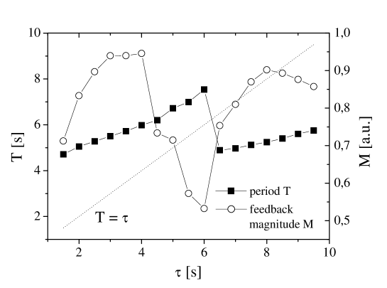
Figure 1: Experimental results on the application of TDAS to the catalytic CO oxidation on Pt(110). Period $T$ of homogeneous oscillations (black squares) and feedback magnitude $M$ (open circles) in dependence on the delay time $\tau$. Reproduced from Ref. [26].

Previously, we showed experimentally [26] that diffusion-induced turbulence could be efficiently suppressed in an oscillatory chemical reaction-diffusion system using TDAS. It was found that the invasiveness of the control scheme could be significantly reduced for an optimized choice of feedback parameters. Figure 1 presents the period of uniform oscillations in the state of control and the feedback magnitude as a function of the delay time in the experiments with CO oxidation on Pt(110). Although the feedback magnitude was significantly reduced for a delay close to $\tau=6$ s, the optimal case of a vanishingly small feedback signal could not be reached. Near the point, for which the period $T$ of stabilized uniform oscillations becomes equal to the delay time $\tau$, an instability was found. As seen in Fig. 1, the system avoids a state corresponding to the intersection point with the line for which $T=\tau$. The stability of this state, for which the feedback vanishes, has been earlier investigated [26] for the uniform system in terms of a phase dynamics equation of a single oscillator. In this article, we extend the analysis to the theoretical study of a spatially extended system.

Since our present work was motivated by the experimental results in [26], we restrict our investigation to the case of a globally applied control signal generated from the averaged complex amplitude. This case is relevant in many experimental situations where a controlled manipulation of the individual system elements is not possible. Note, however, that a different behaviour can be expected for a space dependent application of the control scheme.

3 Linear stability analysis

We choose a superposition of a homogeneous mode $H$ with a small spatially inhomogeneous perturbation of arbitrary non-zero wave number $\kappa$ as an ansatz for the complex oscillation amplitude,

$$\eta(x,t)=H(t)+A_{+}(t)e^{\mbox{\scriptsize i}\kappa x}+A_{-}(t)e^{-\mbox{\scriptsize i}\kappa x}\,.$$ (6)

Substituting expression (6) into Eq. (3), we can separate, for small $A_{\pm}$, homogeneous contributions from the spatially inhomogeneous terms. In this way, we find an equation for the homogeneous mode which is decoupled from the nonuniform contributions,

$$\dot{H}=(1-\mbox{i}\omega)H-(1+\mbox{i}\beta)|H|^{2}H+\mu e^{\mbox{\scriptsize i}\chi}(H(t-\tau)-H(t))\,,$$ (7)

and a pair of coupled equations for the wave amplitudes $A_{\pm}$,

$$\dot{A}_{+} =(1-\mbox{i}\omega)A_{+}-(1+\mbox{i}\varepsilon)\kappa^{2}A_{+}-2(1+ \mbox{i}\beta)|H|^{2}A_{+}-(1+\mbox{i}\beta)H^{2}A_{-}^{*},$$ (8)

$$\dot{A}_{-}^{*} =(1+\mbox{i}\omega)A_{-}^{*}-(1-\mbox{i}\varepsilon)\kappa^{2}A_{-}^{*}-2(1- \mbox{i}\beta)|H|^{2}A_{-}^{*}-(1-\mbox{i}\beta)H^{*2}A_{+}.$$ (9)

Let us first discuss the dynamics of the uniform mode described by Eq. (7). Substituting $H=\rho_{0}\,e^{-\mbox{\scriptsize i}\Omega t}$ into Eq. (7) we obtain the amplitude of uniform oscillations in the presence of TDAS,

$$\rho_{0}=\sqrt{1+\mu(\cos(\chi+\Omega\tau)-\cos\chi)}\,,$$ (10)

and derive the equation

$$\Omega=\omega+\beta+\mu\beta(\cos(\chi+\Omega\tau)-\cos\chi)-\mu(\sin(\chi+\Omega\tau)-\sin\chi)$$ (11)

determining the frequency $\Omega$ of uniform oscillations. Note that without the feedback ($\mu=0$) the system shows uniform oscillations with the frequency $\Omega_{0}=\omega+\beta$.

Figure 2 shows the results of numerical integration of Eq. (7). The oscillation period $T=2\pi/\Omega$ is shown as a function of the delay time $\tau$ for weak and strong feedbacks. We see that the state with $T=\tau$ is stable for a weak feedback and becomes unstable for a high feedback intensity. The strong feedback case [Fig. 2(b)] shows a good qualitative agreement with the experimental data in Fig. 1.

The stability of the state with $T=\tau$ can be understood in terms of the bifurcation diagram presented in Fig. 3. This diagram is constructed by solving Eq. (11) for a delay time $\tau$ equal to the period $T_{0}=2\pi/(\omega+\beta)$ of oscillations in the nonperturbed uniform system. Besides a solution with a vanishing feedback term, for which $\Omega=\Omega_{0}$, other solutions with a non-zero feedback and $\Omega\neq\Omega_{0}$ are yielded by Eq. (11). Linear stability analysis shows that the solution with $\Omega=\Omega_{0}$ and a vanishing feedback is stable for small $\mu$ and becomes unstable beyond some critical feedback intensity $\mu_{0}$. These results are similar to those obtained by using the phase dynamics approximation for a single oscillator in the presence of TDAS [26].

We now turn to the stability analysis of uniform oscillations with respect to spatially inhomogeneous perturbations. The solution of the linear equations (8) and (9) can be sought as $A_{+}=A_{+}^{0}e^{-i\Omega t}e^{\lambda t}$ and $A_{-}^{*}=A_{-}^{*0}e^{i\Omega t}e^{\lambda t}$. Substituting this into (8) and (9), we obtain the following expression

$$\lambda_{1,2}=1-\kappa^{2}-2\rho_{0}^{2}\pm\sqrt{(1+\beta^{2})\rho_{0}^{4}-(\Omega-\omega-\varepsilon\kappa^{2}-2\beta\rho_{0}^{2})^{2}}\,,$$ (12)

where $\rho_{0}$ is given by Eq. (10) and $\Omega$ is a solution of Eq. (11). Uniform oscillations are stable with respect to the growth of spatially nonuniform modes if Re $\lambda_{1,2}<0$ for all wavenumbers $\kappa$. The instability boundary is therefore determined by the conditions

$$\mbox{Re}\,\lambda(\mu_{c},\kappa_{c}) = 0\,,$$ (13)

$$\frac{\partial}{\partial\kappa}\mbox{Re}\,\lambda(\mu_{c},\kappa_{c}) = 0\,.$$ (14)

Here, Eq. (14) accounts for the fact that the wave number of the first unstable mode corresponds to a maximum in $\lambda$ plotted as a function of $\kappa$. The equations (13) and (14) can be solved numerically, taking into account Eq. (11) yielding the dependence of the frequency $\Omega$ of the uniform mode on the feedback intensity $\mu$ and the delay time $\tau$.

We are particularly interested in the stability of uniform oscillations with $\Omega=\Omega_{0}$ and $\tau=T_{0}$. Inserting this into the general expression (12) for $\lambda$, we find

$$\lambda_{1,2}=-\kappa^{2}-1\pm\sqrt{-\varepsilon^{2}\kappa^{4}-2\beta\varepsilon\kappa^{2}+1}\,,$$ (15)

which is independent of $\mu$. Therefore, this state is always unstable when the Benjamin-Feir condition $1+\varepsilon\beta<0$ is fulfilled. All inhomogeneous modes with a wavenumber less than

$$\kappa=\sqrt{-\frac{2(1+\varepsilon\beta)}{1+\varepsilon^{2}}}$$ (16)

are growing, no matter how $\mu$ is chosen. Thus, for $1+\varepsilon\beta<0$ the solution with $\Omega=\omega+\beta$ will be always unstable so that a noninvasive stabilization of uniform oscillations with TDAS is not possible in this type of system.

For the other solutions with $\Omega\neq\Omega_{0}$ at $\tau=T_{0}$, presented in Fig. 3, the feedback signal is nonzero. In this case, we can determine $\mu_{c}$ from the general expression (12) for $\lambda$ by numerically solving equations (13) and (14). Figure 4 shows the critical feedback intensity $\mu_{c}$ as a function of the dispersion parameter $\varepsilon$ for $\tau=T_{0}$ and the other parameters chosen as in Fig. 3. In the Benjamin-Feir unstable regime, $\mu_{c}$ lies above the bifurcation point $\mu_{0}$ at which the solution with $\Omega=\Omega_{0}$ becomes unstable, cf. Fig. 3. As the system approaches the Benjamin-Feir line with decreasing $\varepsilon$, the critical feedback intensity necessary to stabilize uniform oscillations decreases and finally converges towards $\mu_{0}$.

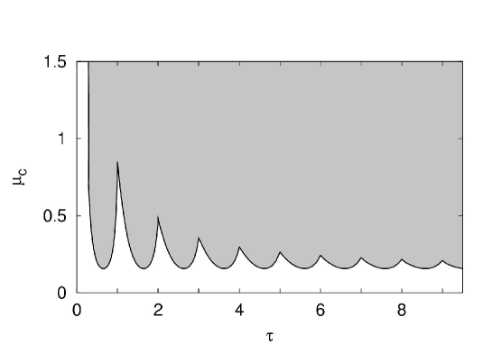
Figure 6: Extended synchronization diagram. The same parameters as in Fig. 5.

From the conditions (13) and (14), we can also determine the critical feedback intensity $\mu_{c}$ as a function of the delay time $\tau$. The resulting synchronization diagram in the plane spanned by the feedback parameters $\tau$ and $\mu$ is displayed in Fig. 5(a). The curve for the critical feedback intensity $\mu_{c}$ divides the plane into a shaded region, where uniform oscillations are linearly stable with respect to small perturbations of arbitrary wavenumber, and a region where uniform osciallations are unstable. The characteristic feature of this diagram is the repeated appearance of cusps. They are observed whenever $\tau$ becomes equal to an integer multiple of the period of the unperturbed uniform system, $\tau=k\,2\pi/(\omega+\beta),k=1,2,3,...$ . Figure 6 shows an extension of the top part of Fig. 5 towards large delay times. With increasing $\tau$, the cusps get less pronounced and the boundary converges to a flat line at $\mu\approx 0.16$.

According to this analytically derived synchronization diagram, stability of uniform oscillations can also be maintained by applying global feedbacks with very large delay times. Moreover, the critical feedback strength, needed to maintain synchronization, does not depend on the delay in the limit $\tau\rightarrow\infty$. To understand this result, we note that the feedback signal $F(t)$ for $\tau\rightarrow\infty$ is given by

$$F(t)=\mu e^{i\chi}\left[\rho_{0}e^{-i(\Omega t+\phi_{0})}-\bar{\eta}(t)\right]$$ (17)

where $\phi_{0}$ is a constant phase shift. The first term here corresponds to the state $\bar{\eta}(t-\tau)$ at $\tau\rightarrow\infty$ which is essentially the initial state of the system. When destabilization of initally uniform oscillations is considered to determine the stability boundary, this initial state represents uniform oscillations with frequency $\Omega$ and amplitude $\rho_{0}$. Substituting this expression for $F(t)$ into Eq. (3), we see that then a situation with external periodic forcing is effectively realized. The critical value $\mu_{c}$ corresponds in this case to the minimum forcing intensity needed to maintain uniform oscillations in the system.

In Fig. 5(b,c), the critical wavenumber and the frequency are shown, respectively, as functions of the delay time along the lower part ABC of the stability boundary. The two curves are of similar shape: they display a decrease for increasing delay time interrupted by discontinuous jumps. These discontinuities occur at the locations where the cusps are found in the stability boundary in Fig. 5(a).

In Fig. 7, we show the real part of $\lambda$ as a function of $\kappa$ at three different points on the stability curve in the ($\mu,\tau$) plane. The three cases correspond to what has been found earlier for a different global delayed feedback scheme in the CGLE [33]. On the branch AB (and similarly also on the branches BC and to the right of C), the first unstable modes occur with a wavenumber $\kappa_{0}\neq 0$ where $\mbox{Im}(\lambda)=0$, see Fig. 7(b,c). Thus, if we cross this branch of the stability boundary by reducing the feedback intensity below the critical value $\mu_{c}$, uniform oscillations will become unstable and standing waves with wavenumber $\kappa_{0}$ will emerge (cf. Sec. 4). A different situation is encountered on the branch reaching from A upwards, see Fig. 7(a). Here, the instability will occur by periodic spatiotemporal modulations of uniform oscillations, since $\mbox{Im}(\lambda)\neq 0$ and the most unstable modes will have wavenumbers close to $\kappa_{0}=0$.

4 Numerical simulations

All simulations were carried out for a one-dimensional system of length $L=128$ on an equidistant grid with $\Delta x=0.32$ (corresponding to a total number of 400 grid points). We use a second-order finite-difference scheme for the discretization of the Laplacian operator and impose periodic boundary conditions. An explicit Euler scheme with a fixed time step of $\Delta t=0.001$ was employed for integration. As initial condition, a uniform state superposed with a small spatially inhomogeneous perturbation was chosen. The set of parameters is as in the previous section: $\varepsilon=2$, $\beta=-1.4$, $\omega=2\pi-\beta\approx 7.68$, and $\chi=\pi/2$. The choice of the feedback parameters $\mu$ and $\tau$ is different for the different simulations and specified below.

In the first series of simulations, we systematically scan the parameters $\mu$ and $\tau$ in steps of $\Delta\mu=\Delta\tau=0.1$ between 0 and 2.5, respectively, to verify the shape of the stability domain in the ($\mu,\tau$) plane. When starting from uniform initial conditions, the stability diagram displayed in Fig. 5(a) is nicely reproduced after transients. Asymptotic states are uniform inside the domain of stability and nonuniform outside this region. These nonuniform states are, however, of different types. Far from the region of stability, we asymptotically reach a fully developed state of defect-mediated turbulence. As the stability boundary is approached, phase turbulence and standing wave patterns are observed close to the branches AB, BC, and to the right of C.

Figure 8 shows the results of a more detailed scan of $\mu$ and $\tau$ in the vicinity of the branch AB of the synchronization diagram in Fig. 5(a). Again, we start from uniform initial conditions. The feedback parameters $\mu$ and $\tau$ are changed in steps of $\Delta\mu=\Delta\tau=0.025$ between $\tau=0.25\,...\,0.975$ and $\mu=0\,...\,0.7$. Simulations that, after transients, resulted in a regular nonuniform spatiotemporal state are marked by bold dots at the corresponding ($\mu,\tau$) coordinates (simulations leading to a uniformly oscillating or turbulent asymptotic states are not shown). Obviously, the parameter region, where regular spatiotemporal patterns occur, constitutes a slightly asymmetric prolongation of the tongue-shaped stability domain for uniform oscillations towards smaller feedback intensities. From the result of the first coarse parameter scan we conjecture, that the regions where spatiotemporal patterns occur look qualitatively similar at the other tongue-shaped branches of the stability curve.

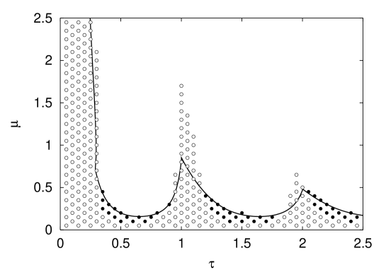
Figure 9: Summary of numerical simulations starting from turbulent initial conditions. Asymptotic states are shown in the ($\mu,\tau$) plane. Open circles denote amplitude turbulence and bold circles indicate regular nonuniform wave patterns. Symbols are omitted in the areas where computations converge to uniform oscillations. The solid line shows the analytically derived stability boundary for uniform initial conditions. The parameters are as in Fig. 5.

When starting from turbulent initial conditions, the stability boundary for uniform oscillations is moved towards larger feedback intensities in the vicinity of the cusps. The results of numerical simulations are summarized in Fig. 9. Here, open circles indicate a turbulent asymptotic state and bold circles again denote the appearance of a regular nonuniform wave pattern. Inside the area where no symbols are shown, simulations converge towards uniform oscillations. For comparison, the analytically derived synchronization diagram from Fig. 5(a) is also displayed.

To get a better idea of how the spatiotemporal dynamics of the system changes in the parameter range between turbulence and uniform oscillations, we show in Fig. 10 a series of spacetime plots of asymptotic dynamical states reached for different feedback intensities at a fixed delay time of $\tau=0.5$. The amplitude $|\eta|$ is plotted in a grey scale color coding and the feedback intensity $\mu$ is increased in Fig. 10 from (a) to (e). In absence of feedback (Fig. 10(a), $\mu=0$) and for small feedback intensities (Fig. 10(b), $\mu=0.05$), an irregular state of defect-mediated turbulence is observed. However, the number of defects is smaller in the presence of a weak feedback and the time evolution shows intervalls, where almost no defects are seen. If the feedback intensity is increased (Fig. 10(c), $\mu=0.07$), defects are no longer observed and the system displays a disordered state of phase turbulence. For even stronger feedback, breathing (Fig. 10(d), $\mu=0.1$) and stationary standing wave patterns (Fig. 10(e), $\mu=0.15$) can be observed. For still larger feedbacks, $\mu>0.2$ (not shown), uniform oscillations take place.

To study the behaviour of the system for very large delays, a series of simulations with the delays $\tau$ varying from 0.5 to 29.5 in steps of $\Delta\tau=1$ has further been performed. The feedback intensity $\mu$ was varied for each choice of $\tau$ from 0.1 to 0.3 in the steps of $\Delta\mu=0.1$. The initial conditions in these simulations represented the state of amplitude turbulence reached by the system if $\mu=0$. These numerical investigations have revealed that synchronization is possible for all chosen delays, when the feedback intensity exceeds a critical level. In another series of experiments, the feedback intensity was fixed at $\mu=1$ and the delay time $\tau$ was increased from 0 to 50 in steps of 0.1. Here, the transient time was determined for each of the simulations by looking at the convergence of the statistical variance of the amplitude $\rho$. It was found that for small delays the transient time increases proportionally to the delay $\tau$. For large delays, the transient time undergoes saturation at a level independent of $\tau$, but depending on the intensity of the applied feedback.

For very long delays $\tau$, the component $\bar{\eta}(t-\tau)$ in the feedback signal $F(t)$ at time $t$ corresponds to the initial state of amplitude turbulence. Thus, the global delayed feedback scheme in the considered limit effectively represents global forcing of the system with an external chaotic signal corresponding to the initial turbulent state in absence of feedback. To verify this conjecture, special numerical simulations have been performed. In these simulations, the feedback signal was generated by replacing $\bar{\eta}(t-\tau)$ with the average complex oscillation amplitude of the same system without the feedback. We have found that, by applying such chaotic external forcing, synchronization of uniform oscillations can also be achieved.

5 Discussion

Motivated by our experiments [26] on control of chemical turbulence in the CO oxidation reaction on Pt(110), we have performed a detailed study of the effects of time-delay autosynchronization on uniform oscillations in a general model described by the complex Ginzburg-Landau equation. We have seen that, like in the experiments, the noninvasive stabilization of uniform oscillations by this method is not possible, though the required magnitude of the feedback signal can be significantly reduced by using an optimal delay time. The obtained synchronization diagram exhibits a series of cusps at the values of delay times equal to integer multiples of the oscillation period of the unperturbed uniform system. This feature seems to be common for various oscillatory systems with delayed coupling and has also been found in the case of the Kuramoto model of phase oscillators with a delayed global coupling [35]. Near the synchronization boundary, the formation of standing waves and a state of modified intermittent turbulence were observed. These effects are similar to those previously discussed for a different feedback scheme [32, 33, 34]. In contrast to our previous studies, the action of feedbacks with long delay times has also been investigated. We have shown that such feedbacks are also capable of synchronizing oscillations and this effect can essentially be explained as suppression of turbulence by external noisy forcing.

6 Figures

Figure 2: Results of numerical integration of Eq.(7). The oscillation period is plotted as a function of the delay time for (a) low ($\mu=0.5$) and (b) high ($\mu=1.0$) feedback intensities. The parameters are $\beta=-1.4$, $\omega=2\pi-\beta\approx 7.68$, and $\chi=\pi/2$.

Figure 3: Bifurcation diagram for $\tau=T_{0}=1$. The parameters are as in Fig. 2. Dotted lines denote unstable branches. The uniform solution with $\Omega=\Omega_{0}=2\pi$ and a vanishing feedback signal undergoes a transcritical bifurcation at $\mu=\mu_{0}$ and becomes unstable.

Figure 4: Critical feedback intensity $\mu_{c}$ for $\tau=T_{0}=1$ as a function of the dispersion coefficient $\varepsilon$ with $\beta=-1.4$. The line $\mu=\mu_{0}$ denotes the feedback intensity for which the transcritical bifurcation occurs in the uniform system (cf. Fig. 3). The other parameters are as in Fig. 2.

Figure 5: (a) Synchronization diagram. Uniform oscillations are stable inside the shaded region. (b,c) The dependences of the critical wavenumber $\kappa_{c}$ and the critical frequency $\Omega_{c}$ on the delay time $\tau$. The parameters are $\varepsilon=2$, $\beta=-1.4$, $\omega=2\pi-\beta\approx 7.68$, and $\chi=\pi/2$.

Figure 7: Growth rate $\mbox{Re}\,\lambda$ of spatially nonuniform modes as a function of wavenumber $\kappa$ at three different points on the stability curve displayed in Fig. 5(a). The parameters are $\tau=0.29$, $\mu=1.29$ (a), $\tau=0.36$, $\mu=0.4$ (b), and $\tau=0.7$, $\mu=0.16$ (c); other parameters as in Fig. 5.

Figure 8: Regular spatiotemporal patterns at the border of complete synchronization for uniform initial conditions. Section of the ($\mu,\tau$) plane with the analytical result for the AB branch of the stability curve (cf. Fig 5) plotted as a solid line. Bold dots mark the parameters where regular spatiotemporal patters are observed.

Figure 10: Spatiotemporal patterns in the parameter region between turbulence and complete synchronization. The amplitude $|\eta|$ is displayed in a grey scale coding, where black (white) denotes low (high) values of the real amplitude. The delay time is kept constant, $\tau=0.5$ s, and the feedback intensity increases from top to bottom, (a) $\mu=0$, (b) $\mu=0.05$, (c) $\mu=0.07$, (d) $\mu=0.1$, and (e) $\mu=0.15$.

References

- [1] M. C. Cross, P. C. Hohenberg, Pattern formation outside of equilibrium, Rev. Mod. Phys. 65 (1993) 851–1112.
- [2] A. S. Mikhailov, Foundations of Synergetics I, Distributed Active Systems, Springer, Berlin, 1994.
- [3] A. Zaikin, A. Zhabotinsky, Concentration wave propagation in two–dimensional liquid–phase self–oscillating system, Nature 225 (1970) 535–537.
- [4] A. Winfree, Spiral waves of chemical activity, Science 175 (1972) 634–636.
- [5] R. Imbihl, G. Ertl, Oscillatory kinetics in heterogeneous catalysis, Chem. Rev. 95 (1995) 697–733.
- [6] E. Schöll, Nonlinear Spatio-Temporal Dynamics and Chaos in Semiconductors, Cambridge University Press, Cambridge, 2001.
- [7] E. Ben-Jacob, I. Cohen, H. Levine, Cooperative self–organization of microorganisms, Adv. Phys. 49 (4) (2000) 395–554.
- [8] Y. Kuramoto, Chemical Oscillations, Waves, and Turbulence, Springer, Berlin, 1984.
- [9] I. S. Aranson, L. Kramer, The world of the complex Ginzburg-Landau equation, Rev. Mod. Phys. 74 (2002) 99–143.
- [10] P. Coullet, L. Gil, J. Lega, Defect-mediated turbulence, Phys. Rev. Lett. 62 (1989) 1619–1622.
- [11] H. Schuster, Handbook of Chaos Control, Wiley-VCH, Weinheim, 1999.
- [12] E. Ott, C. Grebogi, J. A. Yorke, Controlling chaos, Phys. Rev. Lett. 64 (11) (1990) 1196–1199.
- [13] W. L. Ditto, S. N. Rauseo, M. L. Spano, Experimental control of chaos, Phys. Rev. Lett. 65 (1990) 3211–3214.
- [14] T. L. Carroll, I. Triandaf, I. Schwartz, L. Pecora, Tracking unstable orbits in an experiment, Phys. Rev. A 46 (1992) 6189–6192.
- [15] V. Petrov, V. Gáspár, J. Masere, K. Showalter, Controlling chaos in the Belousov-Zhabotinsky reaction, Nature 361 (1993) 240–243.
- [16] K. Pyragas, Continuous control of chaos by self–controlling feedback, Phys. Lett. A 170 (1992) 421–428.
- [17] J. E. S. Socolar, D. W. Sukow, D. J. Gauthier, Stabilizing unstable periodic orbits in fast dynamical systems, Phys. Rev. E 50 (4) (1994) 3245–3248.
- [18] T. Pierre, G. Bonhomme, A. Atipo, Controlling the chaotic regime of nonlinear ionization waves using the time–delay autosynchronization method, Phys. Rev. Lett. 76 (13) (1996) 2290–2293.
- [19] G. Franceschini, S. Bose, E. Schöll, Control of chaotic spatiotemporal spiking by time–delay autosynchronization, Phys. Rev. E 60 (5) (1999) 5426–5434.
- [20] P. Parmananda, R. Madrigal, M. Rivera, L. Nyikos, I. Kiss, V. Gáspár, Stabilization of unstable steady states and periodic orbits in an electrochemical system using delayed–feedback control, Phys. Rev. E 59 (5) (1999) 5266–5271.
- [21] O. Beck, A. Amann, E. Schöll, J. Socolar, W. Just, Comparison of time-delayed feedback schemes for spatiotemporal control of chaos in a reaction-diffusion system with global coupling, Phys. Rev. E 66 (2002) 016213.
- [22] N. Baba, A. Amann, E. Schöll, Giant improvement of time–delayed feedback control by spatio–temporal filtering, Phys. Rev. Lett. 89 (7) (2002) 074101.
- [23] W. Just, S. Popovich, A. Amann, N. Baba, E. Sch ll, Improvement of time-delayed feedback control by periodic modulation: analytical theory of Floquet mode control scheme, Phys. Rev. E 67 (2003) 026222.
- [24] I. Harrington, J. E. S. Socolar, Limitation on stabilizing plane waves via time-delay feedback, Phys. Rev. E 64 (2001) 056206.
- [25] K. A. Montgomery, M. Silber, Feedback control of traveling wave solutions in the complex Ginzburg-Landau equation, Nonlinearity, submitted (cf. http://arxiv.org/abs/nlin.PS/0308021).
- [26] C. Beta, M. Bertram, A. S. Mikhailov, H. H. Rotermund, G. Ertl, Controlling turbulence in a surface chemical reaction by time-delay autosynchronization, Phys. Rev. E 67 (2003) 046224.
- [27] S. Jakubith, H. H. Rotermund, W. Engel, A. v. Oertzen, G. Ertl, Spatiotemporal concentration patterns in a surface reaction: Propagating and standing waves, rotating spirals, and turbulence, Phys. Rev. Lett. 65 (24) (1990) 3013–3016.
- [28] K. Krischer, M. Eiswirth, G. Ertl, Oscillatory CO oxidation on Pt(110): Modeling of temporal self–organization, J. Chem. Phys. 96 (12) (1992) 9161–9172.
- [29] M. Bär, M. Eiswirth, H. Rotermund, G. Ertl, Solitary–wave phenomena in an excitable surface reaction, Phys. Rev. Lett. 69 (6) (1992) 945–948.
- [30] M. Kim, M. Bertram, M. Pollmann, A. v. Oertzen, A. S. Mikhailov, H. H. Rotermund, G. Ertl, Controlling chemical turbulence by global delayed feedback: Pattern formation in catalytic CO oxidation on Pt(110), Science 292 (2001) 1357–1360.
- [31] M. Bertram, C. Beta, M. Pollmann, A. S. Mikhailov, H. H. Rotermund, G. Ertl, Pattern formation on the edge of chaos: Experiments with CO oxidation on a Pt(110) surface under global delayed feedback, Phys. Rev. E 67 (2003) 036208.
- [32] M. Bertram, A. S. Mikhailov, Pattern formation on the edge of chaos: Mathematical modeling of CO oxidation on a Pt(110) surface under global delayed feedback, Phys. Rev. E 67 (2003) 036207.
- [33] D. Battogtokh, A. S. Mikhailov, Controlling turbulence in the complex Ginzburg–Landau equation, Physica D 90 (1996) 84–95.
- [34] D. Battogtokh, A. Preusser, A. S. Mikhailov, Controlling turbulence in the complex Ginzburg–Landau equation II. Two–dimensional systems, Physica D 106 (1997) 327–362.
- [35] M. K. Yeung, S. H. Strogatz, Time delay in the Kuramoto model of coupled oscillators, Phys. Rev. Lett. 83 (1999) 648–651.