Separation of variables and Bäcklund transformations for the symmetric Lagrange top

Abstract.

We construct the 1- and 2-point integrable maps (Bäcklund transformations) for the symmetric Lagrange top. We show that the Lagrange top has the same algebraic Poisson structure that belongs to the $sl(2)$ Gaudin magnet. The 2-point map leads to a real time-discretization of the continuous flow. Therefore, it provides an integrable numerical scheme for integrating the physical flow. We illustrate the construction by few pictures of the discrete flow calculated in MATLAB.

1. Introduction: the symmetric Lagrange top

The Lagrange top is an integrable case of rotation of a rigid body around a fixed point in a homogeneous gravitational field, characterized by the following conditions [2, 4]: the rigid body is rotationally symmetric, i.e. two of its three principal moments of inertia coincide, and the fixed point lies on the axis of the rotational symmetry. A standard form of the corresponding equations of motion is given by the Euler-Poisson equations:

(1.0.1) $$\left\{\begin{array}[]{ll}\dot{J}=P\times x,\\ \dot{x}=J\times x.\end{array}\right.$$

Here $J=(J_{1},J_{2},J_{3})\in\mathbb{R}^{3}$ is the vector of angular momentum of the body, $P=(0,0,\alpha)\in\mathbb{R}^{3}$ is the constant vector along the gravity field and $x=(x_{1},x_{2},x_{3})\in\mathbb{R}^{3}$ is the vector pointing from the fixed point to the center of mass.

The symmetric Lagrange top is an integrable system with 2 degrees of freedom and the Hamiltonian

(1.0.2) $$\mathcal{H}=\frac{1}{2}(J_{1}^{2}+J_{2}^{2}+J_{3}^{2})+\alpha x_{3},$$

where $J_{k},x_{k}$, $k=1,2,3$ are six generators of the Lie-Poisson $e(3)$ algebra defined by the following Poisson brackets:

(1.0.3) $$\{J_{k},J_{l}\}=J_{m},\qquad\{J_{k},x_{l}\}=x_{m},\qquad\{x_{k},x_{l}\}=0,$$

$(klm)$ is a cyclic permutation of $(123)$.

We will also use the complex conjugated variables $J_{\pm}=J_{1}\pm iJ_{2}$ and $x_{\pm}=x_{1}\pm ix_{2}$, which have the brackets

(1.0.4) $$\{J_{3},J_{\pm}\}=\mp iJ_{\pm},\qquad\{J_{+},J_{-}\}=-2iJ_{3},\qquad\{J_{3},x_{\pm}\}=\{x_{3},J_{\pm}\}=\mp ix_{\pm},$$

$$\{J_{+},x_{-}\}=\{x_{+},J_{-}\}=-2ix_{3},\qquad\{J_{3},x_{3}\}=\{J_{+},x_{+}\}=\{J_{-},x_{-}\}=0,$$

$$\{x_{k},x_{l}\}=0,\qquad k,l=\pm,3.$$

The Lie-Poisson bracket (1.0.3) have two Casimir functions

(1.0.5) $$C_{1}\equiv\sum_{k=1}^{3}x_{k}^{2},\qquad C_{2}\equiv\sum_{k=1}^{3}x_{k}J_{k}.$$

Fixing their values one gets a generic symplectic leaf

(1.0.6) $$\mathcal{O}_{c_{1},c_{2}}\equiv\{x,J|\;C_{1}=c_{1},\;C_{2}=c_{2}\},$$

which is a four-dimensional symplectic manifold. Hereafter we take $c_{1}=1$ and $c_{2}=\ell$, corresponding to a unit vector $x$ and a fixed projection $\ell$ of the angular momentum $J$ on the vector $x$.

Two commuting integrals of motion (Hamiltonians) of the symmetric Lagrange top are respectively,

(1.0.7) $$\mathcal{H}=\frac{1}{2}(J_{1}^{2}+J_{2}^{2}+J_{3}^{2})+\alpha x_{3}\qquad\mbox{and}\qquad J_{3},\qquad\{\mathcal{H},J_{3}\}=0.$$

Obviously, the conservation of $J_{3}$ is a direct consequence of the invariance under rotation about the direction of the gravity field. Using complex generators of $e(3)$ we can write the Hamiltonian as

(1.0.8) $$\mathcal{H}=\frac{1}{2}(J_{+}J_{-}+J_{3}^{2})+\alpha x_{3}.$$

2. From the $sl(2)$ Gaudin magnet to the symmetric Lagrange top

The symmetric Lagrange top can be derived from the $sl(2)$ Gaudin magnet [5, 7], which has the $2\times 2$ Lax matrix

(2.0.1) $$L_{\mathcal{G}}(u)=\sum_{j=1}^{n}\frac{1}{u-a_{j}}\left(\begin{array}[]{cc}s_{j}^{3}&s_{j}^{-}\\ s_{j}^{+}&-s_{j}^{3}\end{array}\right)+\alpha\left(\begin{array}[]{cc}1&0\\ 0&-1\end{array}\right)=\begin{pmatrix}A_{\mathcal{G}}(u)&B_{\mathcal{G}}(u)\cr C_{\mathcal{G}}(u)&-A_{\mathcal{G}}(u)\end{pmatrix},$$

(2.0.2) $$A_{\mathcal{G}}(u)=\alpha+\sum_{j=1}^{n}\frac{s_{j}^{3}}{u-a_{j}}\,,\qquad B_{\mathcal{G}}(u)=\sum_{j=1}^{n}\frac{s_{j}^{-}}{u-a_{j}}\,,\qquad C_{\mathcal{G}}(u)=\sum_{j=1}^{n}\frac{s_{j}^{+}}{u-a_{j}}\,,$$

where $a_{j}\in\mathbb{C}$ and $\alpha\in\mathbb{R}$ are the parameters of the model and $u\in\mathbb{C}$ is the spectral parameter. The parameter $\alpha$ has the meaning of magnetic field’s intensity. Local variables $s_{j}^{3},s_{j}^{\pm}$, $j=1,...,n$, are the generators of the direct sum of $n$ $sl(2)$ spins with the following Poisson brackets:

(2.0.3) $$\{{s_{j}^{3},s_{k}^{\pm}\}}=\mp i\delta_{jk}s_{k}^{\pm},\qquad\{{s_{j}^{+},s_{k}^{-}\}}=-2i\delta_{jk}s_{k}^{3}.$$

We denote the Casimir operators (spins) as $s_{j}$:

(2.0.4) $$s_{j}^{2}=(s_{j}^{3})^{2}+s_{j}^{+}s_{j}^{-}.$$

Fixing $s_{j}$’s we go to a symplectic leaf where the Poisson bracket is non-degenerate, so that the symplectic manifold is a collection of $n$ spheres.

The Lax matrix (2.0.1) satisfies the linear $r$-matrix Poisson algebra:

(2.0.5) $$\{{\stackrel{{\scriptstyle 1}}{{L}}_{\mathcal{G}}(u),\stackrel{{\scriptstyle 2}}{{L_{\mathcal{G}}}}(v)\}}=[r(u-v),\stackrel{{\scriptstyle 1}}{{L}}_{\mathcal{G}}(u)+\stackrel{{\scriptstyle 2}}{{L}}_{\mathcal{G}}(v)],\quad\stackrel{{\scriptstyle 1}}{{L}}_{\mathcal{G}}=L_{\mathcal{G}}\otimes\left(\begin{matrix}1&0\cr 0&1\end{matrix}\right),\quad\stackrel{{\scriptstyle 2}}{{L}}_{\mathcal{G}}=\left(\begin{matrix}1&0\cr 0&1\end{matrix}\right)\otimes L_{\mathcal{G}},$$

with the permutation matrix as the $r$ matrix:

(2.0.6) $$r(u-v)=\frac{i}{u-v}\left(\begin{array}[]{cccc}1&0&0&0\\ 0&0&1&0\\ 0&1&0&0\\ 0&0&0&1\end{array}\right).$$

Equation (2.0.5) is equivalent to the following Poisson brackets for the rational functions $A_{\mathcal{G}}(u)$, $B_{\mathcal{G}}(u)$, $C_{\mathcal{G}}(u)$ (2.0.2):

(2.0.7) $$\{A_{\mathcal{G}}(u),A_{\mathcal{G}}(v)\} = \{B_{\mathcal{G}}(u),B_{\mathcal{G}}(v)\}=\{C_{\mathcal{G}}(u),C_{\mathcal{G}}(v)\}=0,$$

(2.0.8) $$\{A_{\mathcal{G}}(u),B_{\mathcal{G}}(v)\} = \frac{i}{u-v}[B_{\mathcal{G}}(v)-B_{\mathcal{G}}(u)],$$

(2.0.9) $$\{A_{\mathcal{G}}(u),C_{\mathcal{G}}(v)\} = \frac{i}{u-v}[C_{\mathcal{G}}(u)-C_{\mathcal{G}}(v)],$$

(2.0.10) $$\{C_{\mathcal{G}}(u),B_{\mathcal{G}}(v)\} = \frac{2i}{u-v}[A_{\mathcal{G}}(u)-A_{\mathcal{G}}(v)].$$

The non-linear dynamics defined by the equations (1.0.1) is linearised on the Jacobian of the hyperelliptic spectral curve $\Gamma_{\mathcal{G}}$ of genus $n-1$,

(2.0.11) $$\Gamma_{\mathcal{G}}:\qquad\det(L_{\mathcal{G}}(u)-v)=0,$$

which can be brought into the form

(2.0.12) $$v^{2}=A_{\mathcal{G}}^{2}(u)+B_{\mathcal{G}}(u)C_{\mathcal{G}}(u)=\alpha^{2}+\sum_{j=1}^{n}\left(\frac{H_{j}}{u-a_{j}}+\frac{s_{j}^{2}}{(u-a_{j})^{2}}\right).$$

The Hamiltonians $H_{j}$ above are given by

(2.0.13) $$H_{j}=\sum_{k\neq j}\frac{2s_{j}^{3}s_{k}^{3}+s_{j}^{+}s_{k}^{-}+s_{j}^{-}s_{k}^{+}}{a_{j}-a_{k}}+2\alpha s_{j}^{3}.$$

These are integrals of motion of the $sl(2)$ Gaudin magnet, which are Poisson commuting:

(2.0.14) $$\{{H_{j},H_{k}\}}=0\qquad j,k=1,...,n.$$

Take a 2-site Gaudin spin chain for which $n=2$ and the phase space is the direct sum of two $sl(2)$ spins. We use the notations $s_{j}^{1}$ and $s_{j}^{2}$ defined by $s_{j}^{\pm}=s_{j}^{1}\pm is_{j}^{2}$. Introduce a new matrix, called $L(u)$, as follows:

(2.0.15) $$L(u)\equiv iL_{\mathcal{G}}^{(n=2)}(u)=\frac{1}{u-a_{1}}\,L_{1}+\frac{1}{u-a_{2}}\,L_{2}+\alpha\left(\begin{array}[]{cc}i&0\\ 0&-i\end{array}\right),$$

where

(2.0.16) $$L_{k}\equiv\left(\begin{array}[]{cc}is_{k}^{3}&s_{k}^{2}+is_{k}^{1}\\ -s_{k}^{2}+is_{k}^{1}&-is_{k}^{3}\end{array}\right)\in su(2),\qquad k=1,2.$$

Let us consider the following Lie algebras’ isomorphism:

(2.0.17) $$su(2)\oplus su(2)\cong o(4).$$

The Inönü-Wigner contraction from the rotation group $O(m+1)$ to the Euclidean group $E(m)$ [9], for $m=3$, allows us to obtain the Lie-Poisson algebra $e(3)$ for the classical Lagrange top, with six generators $J_{k},x_{k}$, $k=\pm,3$.

Let us introduce the contraction parameter $\epsilon\in(0,1]$. Impose in the equation (2.0.15) the coalescence $a_{2}=a_{1}+\epsilon$, $\epsilon\rightarrow 0$ and redefine $u-a_{1}\equiv u$. Then the Lax matrix reads

(2.0.18) $$L(u)=\frac{1}{u}\,(L_{1}+L_{2})+\frac{1}{u^{2}}\,\epsilon L_{2}+\alpha\left(\begin{array}[]{cc}i&0\\ 0&-i\end{array}\right)+O(\epsilon^{2}).$$

In order to have a $2\times 2$ Lax matrix for the Lagrange top we have to control that $L_{1}+L_{2}$ and $\epsilon L_{2}$ play the role of the following matrices respectively:

(2.0.19) $$J\equiv i\left(\begin{array}[]{cc}J_{3}&J_{-}\\ J_{+}&-J_{3}\end{array}\right),\qquad x\equiv i\left(\begin{array}[]{cc}x_{3}&x_{-}\\ x_{+}&-x_{3}\end{array}\right),$$

or, in other words, we have to check the following Poisson morphisms:

(2.0.20) $$s_{1}^{3}+s_{2}^{3}\cong J_{3},\qquad s_{1}^{+}+s_{2}^{+}\cong J_{+},\qquad s_{1}^{-}+s_{2}^{-}\cong J_{-},$$

$$\epsilon s_{2}^{3}\cong x_{3},\qquad\epsilon s_{2}^{+}\cong x_{+},\qquad\epsilon s_{2}^{-}\cong x_{-}.$$

With a direct calculation of Poisson brackets it is possible to prove that morphisms (2.0.20) actually hold.

Therefore we obtain the $2\times 2$ Lax matrix for the Lagrange top

(2.0.21) $$L(u)=\begin{pmatrix}A(u)&B(u)\cr C(u)&-A(u)\end{pmatrix}=i\left(\begin{matrix}\frac{J_{3}}{u}+\frac{x_{3}}{u^{2}}+\alpha&\frac{J_{-}}{u}+\frac{x_{-}}{u^{2}}&\cr\frac{J_{+}}{u}+\frac{x_{+}}{u^{2}}&-\frac{J_{3}}{u}-\frac{x_{3}}{u^{2}}-\alpha\end{matrix}\right),$$

We want to remark that in the Lagrange case the real parameter $\alpha$ describes the gravitational field’s intensity.

The spectral curve of the Lagrange top is the elliptic curve $\Gamma:\;\det(L(u)-v)=0$,

(2.0.22) $$\Gamma:\qquad-v^{2}=\frac{1}{u^{4}}+\frac{2\ell}{u^{3}}+\frac{2\mathcal{H}}{u^{2}}+\frac{2J_{3}}{u}+\alpha^{2}.$$

The Lie algebra contraction $o(4)\rightarrow e(3)$ does not change the $r$-matrix structure of the model, that remains in the form (2.0.5)–(2.0.6) with the Lax matrix given by (2.0.21).

3. Separation of variables

In this Section we construct the simplest separation of variables for the symmetric Lagrange top with the Lax matrix (2.0.21). The details of the approach can be found in [15, 10, 11].

The basic separation has only one pair $(u_{1},v_{1})$ of separation variables belonging to the spectral curve $\Gamma$ (2.0.22). It corresponds to the standard normalisation vector $\alpha_{0}=(1,0)$ and it is defined by the equations

(3.0.1) $$(1,0)(L(u_{1})-v_{1})^{\wedge}=0,$$

where $(\cdot)^{\wedge}$ denotes the adjoint matrix. Equation (3.0.1) is the equation for the pole $(u_{1},v_{1})$ of the Baker-Akhiezer function $\Psi$, which is defined as a properly normalised eigenfunction of the Lax matrix:

(3.0.2) $$L(u)\Psi=v\Psi,\qquad(u,v)\in\Gamma,$$

(3.0.3) $$\alpha_{0}\cdot\Psi=1.$$

It is easy to see that the equation (3.0.1) gives the following separation variables:

(3.0.4) $$B(u_{1})=0,\qquad v_{1}=-A(u_{1}).$$

Explicitly, the pair of the canonical separation variables is

(3.0.5) $$u_{1}=-\frac{x_{-}}{J_{-}}\,,\qquad v_{1}=i\,\frac{J_{-}}{x_{-}}\left(J_{3}-\frac{J_{-}}{x_{-}}x_{3}\right).$$

In order to define the map between the initial and separation variables, one has to add an extra pair of canonical variables. This pair of variables is taken from the asymptotics ($u\rightarrow\infty$) of the elements $A(u)$ and $B(u)$ of the Lax matrix. We obtain

(3.0.6) $$u_{2}=J_{-},\qquad v_{2}=-i\,\frac{J_{3}}{J_{-}}.$$

Indeed, using the Lie-Poisson algebra $e(3)$ (1.0.4), it is easy to check that the new variables are canonical:

(3.0.7) $$\{u_{k},u_{l}\}=\{v_{k},v_{l}\}=0,\qquad\{v_{k},u_{l}\}=\delta_{kl},\qquad k,l=1,2.$$

Remark that the new separation variables $(u_{1},u_{2},v_{1},v_{2})$ are defined in a complex domain. We can write down the complex generators of $e(3)$ in terms of the separation variables:

(3.0.8) $$J_{-} = u_{2},$$

$$J_{+} = -\frac{2\ell}{u_{1}u_{2}}+v_{2}^{2}u_{2}-\frac{1}{u_{1}^{2}u_{2}}-\frac{u_{1}^{2}v_{1}^{2}}{u_{2}},$$

$$J_{3} = iv_{2}u_{2},$$

$$x_{-} = -u_{1}u_{2},$$

$$x_{+} = -\frac{1}{u_{1}u_{2}}-v_{2}^{2}u_{1}u_{2}+2v_{1}v_{2}u_{1}^{2}-\frac{u_{1}^{3}v_{1}^{2}}{u_{2}},$$

$$x_{3} = iu_{1}(u_{1}v_{1}-u_{2}v_{2}).$$

The separation equations are:

(3.0.9) $$\mathcal{H} = u_{1}^{2}\left(i\alpha v_{1}-\frac{v_{1}^{2}}{2}\right)-\frac{\ell}{u_{1}}-\frac{1}{2u_{1}^{2}}-\alpha J_{3}u_{1},$$

(3.0.10) $$J_{3} = iv_{2}u_{2}.$$

One can use the above separation of variables to integrate the model in terms of elliptic functions. Although, because the separation variables are complex, it is not easy to apply the reality conditions. In the next Section we describe the standard integration of the symmetric Lagrange top.

We finish this Section by presenting the canonical separating transform through a generating function.

Let us fix a special representation of the $e(3)$ algebra in terms of the Darboux coordinates $q_{j},p_{j},j=1,2$:

(3.0.11) $$J_{-} = q_{1},$$

$$J_{+} = q_{1}p_{1}^{2}+2q_{2}p_{1}p_{2}-2i\ell p_{1}-2ip_{2},$$

$$J_{3} = -i(q_{1}p_{1}+q_{2}p_{2})-\ell,$$

$$x_{-} = q_{2},$$

$$x_{+} = q_{2}p_{1}^{2}-2ip_{1},$$

$$x_{3} = -iq_{2}p_{1}-1,$$

(3.0.12) $$\{q_{k},q_{l}\}=\{p_{k},p_{l}\}=0,\qquad\{q_{k},p_{l}\}=\delta_{kl},\qquad k,l=1,2.$$

Notice that in this representation the variables $J_{-}$ and $x_{-}$ do not depend on the momenta and the variables $J_{3}$ and $x_{3}$ are linear in the momenta.

Finally, the canonical transformation $(q_{1},q_{2},p_{1},p_{2})\rightarrow(u_{1},u_{2},v_{1},v_{2})$ is defined by the generating function

(3.0.13) $$F(q_{1},q_{2}\mid v_{1},v_{2})=i\,\frac{q_{1}}{q_{2}}+i\ell\ln q_{2}-q_{1}v_{2}+\frac{q_{2}v_{1}}{q_{1}}\,,$$

that is

(3.0.14) $$p_{i}=\frac{\partial F(q_{1},q_{2}\mid v_{1},v_{2})}{\partial q_{i}}\,,\qquad u_{i}=-\frac{\partial F(q_{1},q_{2}\mid v_{1},v_{2})}{\partial v_{i}}\,,\qquad i=1,2.$$

4. Integrating the model

The standard integration of the Lagrange top is performed through Eulerian variables which allow the reduction to one degree of freedom by using the first order integral $J_{3}$ to separate out the angle $\varphi$ and its conjugated momentum $p_{\varphi}$ [1].

Let us introduce the Eulerian angles $(\theta,\varphi)$, $\theta\in[0,\pi]$, $\varphi\in[0,2\pi)$, to parametrize the unit sphere $x_{1}^{2}+x_{2}^{2}+x_{3}^{2}=1$, which together with the conjugated momenta $(p_{\theta},p_{\varphi})$ give a representation of the $e(3)$ generators in terms of Darboux coordinates:

(4.0.1) $$J_{1} = p_{\theta}\cos\varphi+\frac{\ell-p_{\varphi}\cos\theta}{\sin\theta}\,\sin\varphi,\qquad\quad x_{1}=\sin\varphi\sin\theta,$$

$$J_{2} = -p_{\theta}\sin\varphi+\frac{\ell-p_{\varphi}\cos\theta}{\sin\theta}\,\cos\varphi,\qquad\,x_{2}=\cos\varphi\sin\theta,$$

$$J_{3} = p_{\varphi},\qquad\qquad\qquad\qquad\qquad\qquad\qquad x_{3}=\cos\theta,$$

(4.0.2) $$\{p_{\theta},\theta\}=\{p_{\varphi},\varphi\}=1.$$

One immediately arrives at two one-dimensional equations

(4.0.3) $$\mathcal{H} = \frac{p_{\theta}^{2}}{2}+\frac{p_{\varphi}^{2}-2\ell p_{\varphi}\cos\theta+\ell^{2}}{2\sin^{2}\theta}+\alpha\cos\theta,$$

(4.0.4) $$J_{3} = p_{\varphi},$$

which lead to integration of the model in terms of the Weierstrass elliptic function $\wp(x)$. The time evolution of the angles and of their conjugated momenta is the following:

(4.0.5) $$\theta = \arccos\left[\frac{E}{3\alpha}+\wp\left(\sqrt{\frac{\alpha}{2}}\;t\right)\right],$$

$$\varphi = \int\frac{m-2\ell\left[\frac{E}{3\alpha}+\wp\left(\sqrt{\frac{\alpha}{2}}\;t\right)\right]}{1-\left[\frac{E}{3\alpha}+\wp\left(\sqrt{\frac{\alpha}{2}}\;t\right)\right]^{2}}dt,$$

$$p_{\theta} = \frac{d}{dt}\left\{\arccos\left[\frac{E}{3\alpha}+\wp\left(\sqrt{\frac{\alpha}{2}}\;t\right)\right]\right\},$$

$$p_{\varphi} = m.$$

5. Bäcklund transformations (BT’s)

In this paper, following the approach of [13, 14], we look at the Bäcklund transformations (BT’s) for finite-dimensional (Liouville) integrable systems as special canonical transformations, thereby taking a Hamiltonian point of view. Such BT’s are defined as symplectic, or more generally Poisson, integrable maps which are explicit maps (rather than implicit multivalued correspondences) and which can be viewed as time discretizations of particular continuous flows.

The most characteristic properties of such maps are: (i) a BT preserves the same set of integrals of motion as does the continuous flow which it discretizes, (ii) it depends on a Bäcklund parameter $\lambda$ that specifies the corresponding shift on a Jacobian or on a generalized Jacobian [14, 3], and (iii) a spectrality property holds with respect to $\lambda$ and to the conjugate variable $\mu$, which means that the point $(\lambda,\mu)$ belongs to the spectral curve [13, 14]. Explicitness makes these maps purely iterative, while the importance of the parameter $\lambda$ is that it allows for an adjustable discrete time step. The spectrality property is related with the simplecticity of the map [14].

In this paper we construct BT’s for the symmetric Lagrange top starting from the results obtained in [8]. As shown in previous sections, the Lagrange top has the same algebraic Poisson structure that belongs to the Gaudin magnet. This allows to choose the same ansatz for the matrix $M(u)$ that has been used in [8].

We have here to remark that an elegant alternative approach to integrable time discretizations of continuous hamiltonian flows has been carried out by Yu. B. Suris and A.I. Bobenko [6, 16]. In particular, in [6] they construct a discrete time Lagrange top: notice howewer that their discrete Lax matrix is deformed with respect to the continuous one, which is recovered in the limit when the time step goes to zero.

5.1. One-point BT

A (one-point) Bäcklund transformation for the Lagrange top is equivalent to the following similarity transform on the Lax matrix $L(u)$:

(5.1.1) $$L(u)\longmapsto M(u;\lambda)L(u)M^{-1}(u,\lambda)\qquad\forall u,\qquad\lambda\in\mathbb{C},$$

with some non-degenerate $2\times 2$ matrix $M(u,\lambda)$, simply because a BT should preserve the spectrum of $L(u)$. The parameter $\lambda\in\mathbb{C}$ is called a Bäcklund parameter of the transformation. Let us introduce new $~{}\widetilde{}$ -notations for the updated variables:

(5.1.2) $$\widetilde{L}(u)=\begin{pmatrix}\widetilde{A}(u)&\widetilde{B}(u)\cr\widetilde{C}(u)&-\widetilde{A}(u)\end{pmatrix}=i\left(\begin{matrix}\frac{\widetilde{J}_{3}}{u}+\frac{\widetilde{x}_{3}}{u^{2}}+\alpha&\frac{\widetilde{J}_{-}}{u}+\frac{\widetilde{x}_{-}}{u^{2}}&\cr\frac{\widetilde{J}_{+}}{u}+\frac{\widetilde{x}_{+}}{u^{2}}&-\frac{\widetilde{J}_{3}}{u}-\frac{\widetilde{x}_{3}}{u^{2}}-\alpha\end{matrix}\right).$$

We are looking for a Poisson map that intertwines two Lax matrices $L(u)$ and $\widetilde{L}(u)$:

(5.1.3) $$M(u;\lambda)L(u)=\widetilde{L}(u)M(u;\lambda)\qquad\forall u.$$

Let us take

(5.1.4) $$M(u;\lambda)=\left(\begin{array}[]{cc}u-\lambda+pq&p\\ q&1\end{array}\right),\qquad\det M(u;\lambda)=u-\lambda.$$

Let us stress that the number of zeros of $\det M$ is the number of essential Bäcklund parameters. Here the variables $p$ and $q$ are indeterminate dynamical variables.

The ansatz (5.1.4) for the matrix $M$ came from the simplest $L$-operator of the quadratic $r$-matrix algebra

(5.1.5) $$\{{\stackrel{{\scriptstyle 1}}{{L}}(u),\stackrel{{\scriptstyle 2}}{{L}}(v)\}}=[r(u-v),\stackrel{{\scriptstyle 1}}{{L}}(u)\stackrel{{\scriptstyle 2}}{{L}}(v)],$$

with the same $r$-matrix (2.0.6). Notice that we have a peculiar algebraic situation, as in Gaudin models: a Lax matrix which satisfies a linear $r$-matrix algebra requires a $M$ matrix which comes from a quadratic $r$-matrix algebra. Recall that in the Toda lattice [13] and in the DST model [12] both $L$ and $M$ are derived from the same quadratic $r$-matrix algebra. This fact shall show up in the construction of the quantum analogue of these Bäcklund transformations.

Comparing the asymptotics in $u\rightarrow\infty$ in both sides of (5.1.3) we readily get

(5.1.6) $$\widetilde{J}_{3}=J_{3},\qquad p=\frac{J_{-}}{2\alpha}\,,\qquad q=\frac{\widetilde{J}_{+}}{2\alpha}\,.$$

If we want an explicit single-valued map from $L(u)$ to $\widetilde{L}(u)$ we must express $M(u,\lambda)$, and therefore $p$ and $q$, in term of the old variables. To solve this problem we use the spectrality of the BT. As well as the equation (5.1.3) that our map satisfies, it will be parametrized by a point $P=(\lambda,\mu)\in\Gamma$. Notice that there are two points on $\Gamma$, $P=(\lambda,\mu)$ and $Q=(\lambda,-\mu)$, corresponding to the same $\lambda$ and sitting one above the other because of the elliptic involution:

(5.1.7) $$(\lambda,\mu)\in\Gamma:\qquad\det(L(\lambda)-\mu)=0\qquad\Leftrightarrow\qquad\mu^{2}+\det(L(\lambda))=0.$$

As shown in [8], this spectrality property, used as a new datum, produces the formula

(5.1.8) $$q=\frac{A(\lambda)-\mu}{B(\lambda)}=-\frac{C(\lambda)}{A(\lambda)+\mu}\,,$$

where $\lambda$ and $\mu$ are bound by the equation for the elliptic curve

(5.1.9) $$\mu^{2}=-\left(\frac{1}{\lambda^{4}}+\frac{2\ell}{\lambda^{3}}+\frac{2\mathcal{H}}{\lambda^{2}}+\frac{2J_{3}}{\lambda}+\alpha^{2}\right).$$

Now the equation (5.1.3) gives an integrable Poisson map from $L(u)$ to $\widetilde{L}(u)$. The map is parametrized by one point $(\lambda,\mu)\in\Gamma$. Explicitly, it reads

(5.1.10) $$\widetilde{J}_{3} = J_{3},$$

$$\widetilde{J}_{-} = x_{-}+J_{-}(pq-\lambda)-2pJ_{3},$$

$$\widetilde{J}_{+} = 2q\alpha,$$

$$\widetilde{x}_{3} = x_{3}+pJ_{+}-qx_{-}-qJ_{-}(pq-\lambda)+2pqJ_{3},$$

$$\widetilde{x}_{-} = x_{-}(2pq-\lambda)-2px_{3}-p^{2}J_{+}+J_{-}pq(pq-\lambda)-2p^{2}qJ_{3},$$

$$\widetilde{x}_{+} = J_{+}-J_{-}\frac{q}{p}(pq-\lambda)+2qJ_{3}.$$

If we refer to the real generators of $e(3)$ the map takes the following explicit form,

$$\widetilde{J}_{1} = \alpha q+\frac{1}{2}(x_{1}-ix_{2})-\frac{\lambda}{2}(J_{1}-iJ_{2})+\frac{q}{4\alpha}(J_{1}^{2}-J_{2}^{2})+$$

$$+\frac{i}{2\alpha}(J_{2}J_{3}-qJ_{1}J_{2}+iJ_{1}J_{3}),$$

$$\widetilde{J}_{2} = -i\alpha q+\frac{i}{2}(x_{1}+ix_{2})-\frac{i\lambda}{2}(J_{1}+iJ_{2})+\frac{iq}{4\alpha}(J_{1}^{2}-J_{2}^{2})+$$

$$+\frac{1}{2\alpha}(J_{2}J_{3}-qJ_{1}J_{2}-iJ_{1}J_{3}),$$

$$\widetilde{J}_{3} = J_{3},$$

$$\widetilde{x}_{1} = \alpha q\lambda+\frac{1}{2}(J_{1}+iJ_{2})-\frac{q^{2}}{2}(J_{1}-iJ_{2})-\frac{\lambda}{2}(x_{1}-ix_{2})+qJ_{3}+$$

$$+\frac{q}{2\alpha}\left[\frac{\lambda}{2}(J_{2}^{2}-J_{1}^{2})+(J_{1}-iJ_{2})\left(x_{1}-\frac{x_{3}}{q}\right)-ix_{2}(J_{1}+iJ_{2})+i\lambda J_{1}J_{2}\right]+$$

$$+\frac{q}{8\alpha^{2}}\left[qJ_{1}^{2}(J_{1}-3iJ_{2})+qJ_{2}^{2}(J_{2}-3iJ_{1})-\frac{i}{q}(J_{1}-J_{2})^{2}(J_{1}+J_{2})-2J_{3}(J_{1}-iJ_{2})^{2}\right],$$

$$\widetilde{x}_{2} = -i\alpha q\lambda+\frac{i}{2}(J_{1}-iJ_{2})-\frac{iq^{2}}{2}(J_{1}+iJ_{2})-\frac{i\lambda}{2}(x_{1}-ix_{2})-iqJ_{3}+$$

$$+\frac{iq}{2\alpha}\left[\frac{\lambda}{2}(J_{2}^{2}-J_{1}^{2})+(J_{1}-iJ_{2})\left(x_{1}-\frac{x_{3}}{q}\right)-ix_{2}(J_{1}+iJ_{2})+i\lambda J_{1}J_{2}\right]+$$

$$+\frac{iq}{8\alpha^{2}}\left[qJ_{1}^{2}(J_{1}-3iJ_{2})+qJ_{2}^{2}(J_{2}-3iJ_{1})-\frac{i}{q}(J_{1}-J_{2})^{2}(J_{1}+J_{2})-2J_{3}(J_{1}-iJ_{2})^{2}\right],$$

$$\widetilde{x}_{3} = x_{3}-q(x_{1}-ix_{2})+q\lambda(J_{1}-iJ_{2})+$$

$$+\frac{1}{\alpha}\left[\frac{1}{2}(J_{1}^{2}+J_{2}^{2})-\frac{q^{2}}{2}(J_{1}^{2}-J_{2}^{2})-iq(J_{2}J_{3}-qJ_{1}J_{2}+iJ_{1}J_{3})\right],$$

where we have used (5.1.6) to express $p$ in terms of the old variables.

Notice that the above one-point BT is a complex map, so it is a non-physical Bäcklund transformation.

5.2. Symplecticity of the one-point BT

We give a simple proof of symplecticity of the constructed map by finding an explicit generating function of the corresponding canonical transformation from the old to new variables.

First, because the Casimir functions do not change under the map,

(5.2.1) $$x_{3}^{2}+x_{+}x_{-}=\widetilde{x}_{3}^{2}+\widetilde{x}_{+}\widetilde{x}_{-}=1,$$

(5.2.2) $$\frac{1}{2}(J_{+}x_{-}+J_{-}x_{+})+J_{3}x_{3}=\frac{1}{2}(\widetilde{J}_{+}\widetilde{x}_{-}+\widetilde{J}_{-}\widetilde{x}_{+})+\widetilde{J}_{3}\widetilde{x}_{3}=\ell,$$

we can exclude the variables $x_{+},J_{+}$ and $\widetilde{x}_{-},\widetilde{J}_{-}$, using the following substitutions:

(5.2.3) $$x_{+}=\frac{1-x_{3}^{2}}{x_{-}}\,,\qquad\qquad J_{+}=\frac{2\ell}{x_{-}}-\frac{2J_{3}x_{3}}{x_{-}}-\frac{J_{-}}{x_{-}^{2}}\,(1-x_{3}^{2})\,,$$

(5.2.4) $$\widetilde{x}_{-}=\frac{1-\widetilde{x}_{3}^{2}}{\widetilde{x}_{+}}\,,\qquad\qquad\widetilde{J}_{-}=\frac{2\ell}{\widetilde{x}_{+}}-\frac{2\widetilde{J}_{3}\widetilde{x}_{3}}{\widetilde{x}_{+}}-\frac{\widetilde{J}_{+}}{\widetilde{x}_{+}^{2}}\,(1-\widetilde{x}_{3}^{2}).$$

Now we have only four (old and new) independent variables: $x_{-},x_{3},J_{-},J_{3}$ and $\widetilde{x}_{+},\widetilde{x}_{3},\widetilde{J}_{+},\widetilde{J}_{3}$. We write the 1-point BT as a canonical transformation defined by the generating function $F_{\lambda}(x_{-},J_{-}\mid\widetilde{x}_{+},\widetilde{J}_{+})$ written in terms of $x_{-},J_{-}$ and $\widetilde{x}_{+},\widetilde{J}_{+}$:

(5.2.5) $$x_{3} = ix_{-}\,\frac{\partial F_{\lambda}(x_{-},J_{-}\mid\widetilde{x}_{+},\widetilde{J}_{+})}{\partial J_{-}}\,,$$

$$J_{3} = ix_{-}\,\frac{\partial F_{\lambda}(x_{-},J_{-}\mid\widetilde{x}_{+},\widetilde{J}_{+})}{\partial x_{-}}+iJ_{-}\,\frac{\partial F_{\lambda}(x_{-},J_{-}\mid\widetilde{x}_{+},\widetilde{J}_{+})}{\partial J_{-}}\,,$$

$$\widetilde{x}_{3} = i\widetilde{x}_{+}\,\frac{\partial F_{\lambda}(x_{-},J_{-}\mid\widetilde{x}_{+},\widetilde{J}_{+})}{\partial\widetilde{J}_{+}}\,,$$

$$\widetilde{J}_{3} = i\widetilde{x}_{+}\,\frac{\partial F_{\lambda}(x_{-},J_{-}\mid\widetilde{x}_{+},\widetilde{J}_{+})}{\partial\widetilde{x}_{+}}+i\widetilde{J}_{+}\,\frac{\partial F_{\lambda}(x_{-},J_{-}\mid\widetilde{x}_{+},\widetilde{J}_{+})}{\partial\widetilde{J}_{+}}\,.$$

With the help of (5.1.6) we rewrite equations (5.1.10) of the map in the form

(5.2.6) $$x_{3} = \frac{x_{-}\widetilde{J}_{+}}{2\alpha}+k,\qquad\qquad k^{2}=1+\lambda x_{-}\widetilde{x}_{+},$$

$$J_{3} = \frac{\ell}{k}+\frac{\lambda}{2k}\,(J_{-}\widetilde{x}_{+}+x_{-}\widetilde{J}_{+})-\frac{x_{-}\widetilde{x}_{+}}{2k}+\frac{J_{-}\widetilde{J}_{+}}{2\alpha}\,,$$

$$\widetilde{x}_{3} = \frac{J_{-}\widetilde{x}_{+}}{2\alpha}+k,$$

$$\widetilde{J}_{3} = J_{3}.$$

It is now easy to check that the function

(5.2.7) $$F_{\lambda}(x_{-},J_{-}\mid\widetilde{x}_{+},\widetilde{J}_{+})=-i\,\frac{J_{-}\widetilde{J}_{+}}{2\alpha}-ik\left(\frac{J_{-}}{x_{-}}+\frac{\widetilde{J}_{+}}{\widetilde{x}_{+}}-\frac{1}{\lambda}\right)+i\ell\log{\frac{1+k}{1-k}}-i\alpha\lambda,$$

solves the equations (5.2.5)–(5.2.6). Symplecticity of the map is therefore proven.

Alternatively, we can derive (5.2.7) directly from the generating function constructed for the $sl(2)$ Gaudin magnet in [8]. The one-point BT in that case is given by

(5.2.8) $$s_{j}^{3}=is_{j}^{-}\,\frac{\partial F_{\lambda}(s_{1}^{-},...,s_{n}^{-}\mid\widetilde{s}_{1}{}^{+},...,\widetilde{s}_{n}{}^{+})}{\partial s_{j}^{-}}\,,\qquad\widetilde{s}_{j}{}^{3}=i\widetilde{s}_{j}{}^{+}\,\frac{\partial F_{\lambda}(s_{1}^{-},...,s_{n}^{-}\mid\widetilde{s}_{1}{}^{+},...,\widetilde{s}_{n}{}^{+})}{\partial\widetilde{s}_{j}{}^{+}}\,,$$

where

(5.2.9) $$F_{\lambda}(s_{1}^{-},...,s_{n}^{-}\mid\widetilde{s}_{1}{}^{+},...,\widetilde{s}_{n}{}^{+})=-\frac{i}{2\alpha}\sum_{j,k=1}^{n}s_{j}^{-}\widetilde{s}_{k}{}^{+}-i\sum_{j=1}^{n}\left(2z_{j}+s_{j}\log{\frac{z_{j}-s_{j}}{z_{j}+s_{j}}}\right)-i\alpha\lambda,$$

(5.2.10) $$z_{j}^{2}=s_{j}^{2}-(a_{j}-\lambda)\widetilde{s}_{j}{}^{+}s_{j}^{-},\qquad s_{j}^{2}=(s_{j}^{3})^{2}+s_{j}^{-}s_{j}^{+}=(\widetilde{s}_{j}{}^{3})^{2}+\widetilde{s}_{j}{}^{-}\widetilde{s}_{j}{}^{+},\qquad j=1,\ldots,n.$$

Set $n=2$ in (5.2.9) and impose the coalescence $a_{2}=a_{1}+\epsilon$, $\epsilon\rightarrow 0$, similar to the derivation of the Lax matrix for the Lagrange top in Section 2. Now redefine $\lambda-a_{1}\equiv\lambda$ and obtain

(5.2.11) $$\mathcal{F}_{\lambda}(s_{1}^{-},s_{2}^{-}\mid\widetilde{s}_{1}{}^{+},\widetilde{s}_{2}{}^{+})=-\frac{i}{2\alpha}\sum_{j,k=1}^{2}s_{j}^{-}\widetilde{s}_{k}{}^{+}-i\sum_{j=1}^{2}\left(2\zeta_{j}+s_{j}\log{\frac{\zeta_{j}-s_{j}}{\zeta_{j}+s_{j}}}\right)-i\frac{\zeta_{2}}{\lambda}\epsilon-i\alpha\lambda+O(\epsilon^{2}),$$

where

(5.2.12) $$\zeta_{j}^{2}=s_{j}^{2}+\lambda\widetilde{s}_{j}{}^{+}s_{j}^{-},\qquad\qquad j=1,2.$$

Referring to the formulae (2.0.20) we easily deduce that

(5.2.13) $$\zeta_{1}^{2}=s_{1}^{2}+\lambda\left(J_{-}\widetilde{J}_{+}-\frac{\widetilde{J}_{+}x_{-}+J_{-}\widetilde{x}_{+}}{\epsilon}-\frac{x_{-}\widetilde{x}_{+}}{\epsilon^{2}}\right),\quad s_{1}^{2}=J_{3}^{2}+J_{+}J_{-}-\frac{2\ell}{\epsilon}+\frac{1}{\epsilon^{2}}\,,$$

(5.2.14) $$\zeta_{2}^{2}=s_{2}^{2}(1+\lambda x_{-}\widetilde{x}_{+}),\qquad s_{2}^{2}=\frac{1}{\epsilon^{2}}\,.$$

Now it is easy to check that (5.2.11) with (5.2.13)–(5.2.14) coincides with the generating function (5.2.7).

5.3. Spectrality of the one-point BT

The spectrality property of a Bäcklund transformation [13] means that the two components, $\lambda$ and $\mu$, of the point $(\lambda,\mu)\in\Gamma$ parametrizing the map are conjugated variables, in the sense that

(5.3.1) $$\mu=-\frac{\partial F}{\partial\lambda}\,,$$

where $F$ is the generating function of the BT.

We now show the spectrality property for the one-point BT constructed in the previous section. Using the equations (5.1.6), (5.1.8), (5.2.6) and (5.2.7) we obtain

$$\mu = A(\lambda)-\frac{\widetilde{J}_{+}}{2\alpha}\,B(\lambda)=\frac{i}{k}\left[\frac{1}{\lambda^{2}}+\frac{\ell}{\lambda}+\frac{x_{-}\widetilde{x}_{+}}{2}\left(\frac{J_{-}}{x_{-}}+\frac{\widetilde{J}_{+}}{\widetilde{x}_{+}}-\frac{1}{\lambda}\right)+\alpha k\right]=$$

$$= -\frac{\partial F_{\lambda}(x_{-},J_{-}\mid\widetilde{x}_{+},\widetilde{J}_{+})}{\partial\lambda}\,.$$

5.4. One-point BT in Eulerian variables

As shown in Section 4 one can represent the Lie-Poisson algebra $e(3)$ using the canonical realization (4.0.1). Now we rewrite the one-point BT as a canonical map in terms of these variables

(5.4.1) $$\mathcal{B}_{\lambda}:\quad(\theta,\varphi,p_{\theta},p_{\varphi})\longmapsto(\widetilde{\theta},\widetilde{\varphi},\widetilde{p}_{\theta},\widetilde{p}_{\varphi}),$$

where tilde refers to the updated versions of the generators

(5.4.2) $$\widetilde{J}_{1} = \widetilde{p}_{\theta}\cos\widetilde{\varphi}+\frac{\ell-\widetilde{p}_{\varphi}\cos\widetilde{\theta}}{\sin\widetilde{\theta}}\,\sin\widetilde{\varphi},\qquad\quad\widetilde{x}_{1}=\sin\widetilde{\varphi}\sin\widetilde{\theta},$$

$$\widetilde{J}_{2} = -\widetilde{p}_{\theta}\sin\widetilde{\varphi}+\frac{\ell-\widetilde{p}_{\varphi}\cos\widetilde{\theta}}{\sin\widetilde{\theta}}\,\cos\widetilde{\varphi},\qquad\,\widetilde{x}_{2}=\cos\widetilde{\varphi}\sin\widetilde{\theta},$$

$$\widetilde{J}_{3} = \widetilde{p}_{\varphi},\qquad\qquad\qquad\qquad\qquad\qquad\qquad\widetilde{x}_{3}=\cos\widetilde{\theta},$$

(5.4.3) $$\{\widetilde{p}_{\theta},\widetilde{\theta}\}=\{\widetilde{p}_{\varphi},\widetilde{\varphi}\}=1.$$

Recall that we have fixed the values of the two Casimir functions as follows: $\sum_{k=1}^{3}x_{k}^{2}=1$ and $\sum_{k=1}^{3}x_{k}J_{k}=\ell$. Using the equations (5.2.6) we can write down the one-point BT as:

(5.4.4) $$\qquad\;\;p_{\varphi} = \frac{1}{k}\left[\ell+\lambda\alpha(\cos\theta+\cos\widetilde{\theta})+\frac{k^{2}-1}{2\lambda}\right]+2\alpha\lambda\left[\frac{(\cos\theta-1)(\cos\widetilde{\theta}-1)}{k^{2}-1}-1\right],$$

$$\widetilde{p}_{\varphi} = p_{\varphi},$$

(5.4.5) $$p_{\theta} = \frac{i}{\sin\theta}\,(\ell-p_{\varphi}\cos\theta)-\frac{2i\alpha\lambda\sin\theta(\cos\widetilde{\theta}-k)}{k^{2}-1}\,,$$

$$\widetilde{p}_{\theta} = \frac{i}{\sin\widetilde{\theta}}\,(p_{\varphi}\cos\widetilde{\theta}-\ell)+\frac{2i\alpha\lambda\sin\widetilde{\theta}(\cos\theta-k)}{k^{2}-1}\,,$$

with

(5.4.6) $$k^{2}=1+\lambda\phi\widetilde{\phi}\sin\theta\sin\widetilde{\theta},\qquad\phi\equiv e^{i\varphi},~{}\;\;\widetilde{\phi}\equiv e^{-i\widetilde{\varphi}}.$$

Remark that in the last formula we have introduced two new variables $\phi$ and $\widetilde{\phi}$: it is a convenient choice since the map depends only on $e^{i\varphi}$ and $e^{-i\widetilde{\varphi}}$.

We want to focus our attention upon the symmetry of the canonical transform (5.4.4)–(5.4.5), which is symmetric under the exchange $(\theta,\varphi)\leftrightarrow(-\widetilde{\theta},-\widetilde{\varphi})$. Notice that the $\phi,\widetilde{\phi}$ dependence is trivial: it involves only the product $\phi\widetilde{\phi}$ (i.e. $\varphi-\widetilde{\varphi}$), which is symmetric under the change $\phi\leftrightarrow\widetilde{\phi}$. The dependence upon $\theta,\widetilde{\theta}$ is more interesting. Let us introduce the exchange operator $\mathcal{P}_{\theta,\widetilde{\theta}}$ such that

(5.4.7) $$\mathcal{P}_{\theta,\widetilde{\theta}}f(\theta,\widetilde{\theta})=f(\widetilde{\theta},\theta),\qquad\mathcal{P}_{\theta,\widetilde{\theta}}^{2}=1,$$

where $f(\theta,\widetilde{\theta})$ is a generic function. For instance we notice that $\mathcal{P}_{\theta,\widetilde{\theta}}k=k$, where $k$ is the function in (5.4.6). If we consider formulae (5.4.4)–(5.4.5) it is easy to notice that

(5.4.8) $$\mathcal{P}_{\theta,\widetilde{\theta}}\,p_{\varphi}=p_{\varphi},\qquad\mathcal{P}_{\theta,\widetilde{\theta}}\,p_{\theta}=-\widetilde{p}_{\theta}.$$

Our aim is to write down the canonical transform in the following form:

(5.4.9) $$p_{\theta}=\frac{\partial F_{\lambda}(\theta,\phi|\widetilde{\theta},\widetilde{\phi})}{\partial\theta}\,,\quad\widetilde{p}_{\theta}=-\frac{\partial F_{\lambda}(\theta,\phi|\widetilde{\theta},\widetilde{\phi})}{\partial\widetilde{\theta}}\,,$$

$$p_{\varphi}=i\phi\frac{\partial F_{\lambda}(\theta,\phi|\widetilde{\theta},\widetilde{\phi})}{\partial\phi}\,,\quad\widetilde{p}_{\varphi}=i\widetilde{\phi}\frac{\partial F_{\lambda}(\theta,\phi|\widetilde{\theta},\widetilde{\phi})}{\partial\widetilde{\phi}}\,,$$

where $F_{\lambda}(\theta,\phi|\widetilde{\theta},\widetilde{\phi})$ is the generating function of the one-point BT. Since equations (5.4.8) hold the immediate consequence is that

(5.4.10) $$F_{\lambda}(\theta,\phi|\widetilde{\theta},\widetilde{\phi})=\mathcal{P}_{\theta,\widetilde{\theta}}F_{\lambda}(\theta,\phi|\widetilde{\theta},\widetilde{\phi})=F_{\lambda}(\widetilde{\theta},\widetilde{\phi}|\theta,\phi).$$

It is possible to prove that the generating function is:

(5.4.11) $$F_{\lambda}(\theta,\phi|\widetilde{\theta},\widetilde{\phi})=-i\alpha\lambda(2\ln\phi\widetilde{\phi}+1)+A_{\lambda}(\theta,\phi|\widetilde{\theta},\widetilde{\phi})+\mathcal{P}_{\theta,\widetilde{\theta}}A_{\lambda}(\theta,\phi|\widetilde{\theta},\widetilde{\phi}),$$

where

(5.4.12) $$A_{\lambda}(\theta,\phi|\widetilde{\theta},\widetilde{\phi})=a_{0}+a_{1}E(\xi|\eta)+a_{2}F(\xi|\eta)+a_{3}\Pi(\zeta;\xi|\eta)$$

with

(5.4.13) $$\left\{\begin{array}[]{llll}a_{0}&=&i\ell\ln\left(\frac{\sin\theta}{\cos\theta+1}\right)-i\frac{k}{2\lambda}+\frac{1}{2}i\ell\ln\left(\frac{1+k}{1-k}\right)+2i\alpha\lambda\left\{\ln(\sin\theta)(1+\cos\widetilde{\theta})-k+\right.\\ &&\left.+\frac{k^{2}-2}{k^{2}-1}\cos\theta+\frac{k}{2(k^{2}-1)}(1+\cos\theta\cos\widetilde{\theta})+\frac{\theta\sin\theta\sin^{2}\widetilde{\theta}}{(k^{2}-1)(\cos\widetilde{\theta}-1)}+\ln\left(\frac{\sin\theta}{\cos\theta+1}\right)+\right.\\ &&+\left.\frac{1}{2}\cos\theta\ln\left(\frac{1+k}{1-k}\right)+\frac{3}{4}\ln\left(\frac{k+1}{k-1}\right)\right\},\\ &&\\ a_{1}&=&\frac{2i\alpha S}{k\cos\theta}\left[(1+\cos\widetilde{\theta})\left(3\lambda-\frac{1}{\phi^{2}\widetilde{\phi}^{2}\sin^{2}\widetilde{\theta}}\right)-\frac{2}{\lambda\phi^{2}\widetilde{\phi}^{2}(1-\cos\widetilde{\theta})}\right],\\ &&\\ a_{2}&=&\frac{2i\alpha S}{k\cos\theta}\left[\frac{2}{\lambda\phi^{2}\widetilde{\phi}^{2}(1-\cos\widetilde{\theta})}-(1+\cos\widetilde{\theta})\left(3\lambda+\frac{1}{\phi\widetilde{\phi}\sin\widetilde{\theta}}\right)\right],\\ &&\\ a_{3}&=&2i\alpha\lambda S\frac{(1-\cos\widetilde{\theta})(k^{2}-1+\sin\theta)}{k\cos\theta\sin\theta}\,,\\ \end{array}\right.$$

(5.4.14) $$\left\{\begin{array}[]{lll}E(\xi|\eta)&=&\int_{0}^{\xi}(1-\sin^{2}\eta\sin^{2}z)^{1/2}dz,\\ &&\\ F(\xi|\eta)&=&\int_{0}^{\xi}(1-\sin^{2}\eta\sin^{2}z)^{-1/2}dz,\\ &&\\ \Pi(\zeta;\xi|\eta)&=&\int_{0}^{\xi}(1-\zeta^{2}\sin^{2}z)^{-1}(1-\sin^{2}\eta\sin^{2}z)^{-1/2}dz,\\ \end{array}\right.$$

(5.4.15) $$\left\{\begin{array}[]{llll}S&=&\frac{k\cos\theta(k^{2}-1)}{k^{2}-2k+\cos^{2}\theta}\sqrt{\sin\theta(k-1-\sin\theta)}\,,\\ &&\\ \xi&=&k\sqrt{\frac{\sin\theta}{k^{2}-1+\sin\theta}}\,,\\ &&\\ \eta&=&\sqrt{-\frac{k^{2}-1+\sin\theta}{k^{2}-1-\sin\theta}}\,,\\ &&\\ \zeta&=&\frac{k^{2}-1+\sin\theta}{\sin\theta}\,.\end{array}\right.$$

In the zero-field case ($\alpha=0$) the generating function simply reads:

(5.4.16) $$F_{\lambda}^{(\alpha=0)}(\theta,\phi|\widetilde{\theta},\widetilde{\phi})=i\ell\ln\left[\frac{1+k}{1-k}\frac{\sin\theta\sin\widetilde{\theta}}{(\cos\theta+1)(\cos\widetilde{\theta}+1)}\right]-i\,\frac{k}{\lambda}\,.$$

5.5. Two-point BT

According to [8], we now construct a composite map which is a product of the map $\mathcal{B}_{P_{1}}\equiv\mathcal{B}_{(\lambda_{1},\mu_{1})}$ and $\mathcal{B}_{Q_{2}}\equiv\mathcal{B}_{(\lambda_{2},-\mu_{2})}$:

(5.5.1) $$\mathcal{B}_{P_{1},Q_{2}}=\mathcal{B}_{Q_{2}}\circ\mathcal{B}_{P_{1}}:~{}L(u)\stackrel{{\scriptstyle\mathcal{B}_{P_{1}}}}{{\longmapsto}}\widetilde{L}(u)\stackrel{{\scriptstyle\mathcal{B}_{Q_{2}}}}{{\longmapsto}}\stackrel{{\scriptstyle\approx}}{{L}}(u).$$

Two maps are inverse to each other when $\lambda_{1}=\lambda_{2}$ and $\mu_{1}=\mu_{2}$. This two-point BT for the Lagrange top is defined by the following ‘discrete-time’ Lax equation:

(5.5.2) $$M(u;\lambda_{1},\lambda_{2})L(u)=\stackrel{{\scriptstyle\approx}}{{L}}(u)M(u;\lambda_{1},\lambda_{2})\qquad\forall u,\qquad\lambda_{1},\lambda_{2}\in\mathbb{C},$$

where the matrix $M(u;\lambda_{1},\lambda_{2})$ is

(5.5.3) $$M(u;\lambda_{1},\lambda_{2})=\begin{pmatrix}u-\lambda_{1}+xX&X\cr-x^{2}X+(\lambda_{1}-\lambda_{2})x&u-\lambda_{2}-xX\end{pmatrix},$$

(5.5.4) $$\det M(u;\lambda_{1},\lambda_{2})=(u-\lambda_{1})(u-\lambda_{2}).$$

Spectrality property with respect to two fixed points $(\lambda_{1},\mu_{1})\in\Gamma$ and $(\lambda_{2},\mu_{2})\in\Gamma$ give

(5.5.5) $$x=\frac{A(\lambda_{1})-\mu_{1}}{B(\lambda_{1})}=-\frac{C(\lambda_{1}}{A(\lambda_{1})+\mu_{1}}=\frac{\stackrel{{\scriptstyle\approx}}{{A}}(\lambda_{2})-\mu_{2}}{\stackrel{{\scriptstyle\approx}}{{B}}(\lambda_{2})}=-\frac{\stackrel{{\scriptstyle\approx}}{{C}}(\lambda_{2})}{\stackrel{{\scriptstyle\approx}}{{A}}(\lambda_{2})+\mu_{2}}=\frac{\widetilde{J}_{+}}{2\alpha}\,,$$

$$X = \frac{(\lambda_{2}-\lambda_{1})B(\lambda_{1})B(\lambda_{2})}{B(\lambda_{1})(A(\lambda_{2})+\mu_{2})-B(\lambda_{2})(A(\lambda_{1})-\mu_{1})}$$

$$= \frac{(\lambda_{1}-\lambda_{2})(A(\lambda_{1})+\mu_{1})(A(\lambda_{2})-\mu_{2})}{(A(\lambda_{1})+\mu_{1})C(\lambda_{2})-(A(\lambda_{2})-\mu_{2})C(\lambda_{1})}$$

$$= \frac{(\lambda_{2}-\lambda_{1})\stackrel{{\scriptstyle\approx}}{{B}}(\lambda_{1})\stackrel{{\scriptstyle\approx}}{{B}}(\lambda_{2})}{\stackrel{{\scriptstyle\approx}}{{B}}(\lambda_{2})(\stackrel{{\scriptstyle\approx}}{{A}}(\lambda_{1})+\mu_{1})-\stackrel{{\scriptstyle\approx}}{{B}}(\lambda_{1})(\stackrel{{\scriptstyle\approx}}{{A}}(\lambda_{2})-\mu_{2})}$$

$$= \frac{(\lambda_{1}-\lambda_{2})(\stackrel{{\scriptstyle\approx}}{{A}}(\lambda_{1})-\mu_{1})(\stackrel{{\scriptstyle\approx}}{{A}}(\lambda_{2})+\mu_{2})}{(\stackrel{{\scriptstyle\approx}}{{A}}(\lambda_{2})+\mu_{2})\stackrel{{\scriptstyle\approx}}{{C}}(\lambda_{1})-(\stackrel{{\scriptstyle\approx}}{{A}}(\lambda_{1})-\mu_{1})\stackrel{{\scriptstyle\approx}}{{C}}(\lambda_{2})}$$

$$= \frac{J_{-}-\stackrel{{\scriptstyle\approx}}{{J}}_{-}}{2\alpha}\,.$$

Now we have two Bäcklund parameters $\lambda_{1},\lambda_{2}\in\mathbb{C}$. The above formulae give several equivalent expressions for the variables $x$ and $X$ since the points $(\lambda_{1},\mu_{1})$ and $(\lambda_{2},\mu_{2})$ belong to the spectral curve $\Gamma$, i.e., are bound by the following relations

(5.5.7) $$\mu_{k}^{2}=A^{2}(\lambda_{k})+B(\lambda_{k})C(\lambda_{k})=\stackrel{{\scriptstyle\approx}}{{A}}^{2}(\lambda_{k})+\stackrel{{\scriptstyle\approx}}{{B}}(\lambda_{k})\stackrel{{\scriptstyle\approx}}{{C}}(\lambda_{k}),\qquad k=1,2.$$

Together with (5.5.5)–(5.5), the formula (5.5.2) give an explicit two-point Poisson integrable map from $L(u)$ to $\stackrel{{\scriptstyle\approx}}{{L}}(u)$ (as well as its inverse, i.e the map from $\stackrel{{\scriptstyle\approx}}{{L}}(u)$ to $L(u)$). The map is parametrized by two points $\mathcal{B}_{P_{1}}\equiv\mathcal{B}_{(\lambda_{1},\mu_{1})}$ and $\mathcal{B}_{Q_{2}}\equiv\mathcal{B}_{(\lambda_{2},-\mu_{2})}$. Let us introduce the notation

(5.5.8) $$\Delta\lambda=\lambda_{1}-\lambda_{2},\qquad\qquad\lambda_{0}=\frac{\lambda_{1}+\lambda_{2}}{2}\,.$$

The map explicitly reads:

(5.5.9) $$\stackrel{{\scriptstyle\approx}}{{J}}_{3}=J_{3},\qquad\stackrel{{\scriptstyle\approx}}{{J}}_{-}=J_{-}-2X,\qquad\stackrel{{\scriptstyle\approx}}{{J}}_{+}=J_{+}+2x(\Delta\lambda-xX),$$

$$\stackrel{{\scriptstyle\approx}}{{x}}_{3} = x_{3}-\alpha(\Delta\lambda-xX)J_{-}+XJ_{+}+2xX(\Delta\lambda-xX),$$

$$\stackrel{{\scriptstyle\approx}}{{x}}_{-} = x_{-}+(2xX+\Delta\lambda)J_{-}-2XJ_{3}-2X\left(xX+\lambda_{0}-\frac{\Delta\lambda}{2}\right),$$

$$\stackrel{{\scriptstyle\approx}}{{x}}_{+} = x_{+}-(2xX+\Delta\lambda)J_{+}+2x(\Delta\lambda-xX)J_{3}-2x(\Delta\lambda-xX)\left(xX-\lambda_{0}-\frac{\Delta\lambda}{2}\right).$$

It is useful to write down the Bäcklund map in terms of the real generators of $e(3)$:

(5.5.10) $$\stackrel{{\scriptstyle\approx}}{{J}}_{1}=J_{1}+x\Delta\lambda-X(1+x^{2}),\qquad\stackrel{{\scriptstyle\approx}}{{J}}_{2}=J_{2}-i\left[x\Delta\lambda+X(1-x^{2})\right],\qquad\stackrel{{\scriptstyle\approx}}{{J}}_{3}=J_{3},$$

$$\stackrel{{\scriptstyle\approx}}{{x}}_{1} = x_{1}-iJ_{2}(2xX-\Delta\lambda)+J_{3}\left[x\Delta\lambda-X(1+x^{2})\right]-$$

$$-\left\{xX^{2}(1+x^{2})+X\left[\lambda_{0}-\frac{\Delta\lambda}{2}-x^{2}\left(\lambda_{0}+\frac{3\Delta\lambda}{2}\right)\right]+x\Delta\lambda\left(\lambda_{0}+\frac{\Delta\lambda}{2}\right)\right\},$$

$$\stackrel{{\scriptstyle\approx}}{{x}}_{2} = x_{2}+iJ_{1}(2xX-\Delta\lambda)-iJ_{3}\left[x\Delta\lambda+X(1-x^{2})\right]-$$

$$-i\left\{xX^{2}(1-x^{2})+X\left[\lambda_{0}-\frac{\Delta\lambda}{2}+x^{2}\left(\lambda_{0}+\frac{3\Delta\lambda}{2}\right)\right]-x\Delta\lambda\left(\lambda_{0}+\frac{\Delta\lambda}{2}\right)\right\},$$

$$\stackrel{{\scriptstyle\approx}}{{x}}_{3} = x_{3}-J_{1}\left[x\Delta\lambda-X(1+x^{2})\right]+iJ_{2}\left[x\Delta\lambda+X(1-x^{2})\right]-2xX(xX-\Delta\lambda).$$

Obviously, when $\lambda_{1}=\lambda_{2}$ (and $\mu_{1}=\mu_{2}$) the map turns into an identity map. With a direct calculation one can show that the map (5.5.10) sends real variables to real variables provided

(5.5.11) $$\lambda_{1}=\bar{\lambda}_{2}\equiv\lambda\in\mathbb{C}.$$

Therefore, the two-point map leads to a physical Bäcklund transformation with two real parameters.

5.6. Two-point BT as a discrete-time map

The two point BT constructed above is a one-parameter ($\lambda_{1}$) time discretization of a family of flows parametrized by the point $Q_{2}=(\lambda_{2},-\mu_{2})$, with the difference $\Delta\lambda$ playing the role of a time step. Recall that the physical time step is $i\Delta\lambda$ since $\Delta\lambda\in i\mathbb{R}$.

Consider the limit

(5.6.1) $$i\Delta\lambda=i(\lambda_{1}-\lambda_{2})=\epsilon,\qquad\epsilon\rightarrow 0.$$

It is easy to see from the formulae of the previous section that

(5.6.2) $$x = x_{0}+O(\epsilon),\qquad x_{0}=\frac{A(\lambda_{2})-\mu_{2}}{B(\lambda_{2})}=-\frac{C(\lambda_{2})}{A(\lambda_{2})+\mu_{2}}\,,$$

$$X = \epsilon X_{0}+O(\epsilon^{2}),\qquad X_{0}=\frac{iB(\lambda_{2})}{2\mu_{2}}\,.$$

The matrix $M$ has the following asymptotics:

(5.6.3) $$M(u;\lambda_{2})=(u-\lambda_{2})\left[1+\frac{i\epsilon}{2\mu_{2}(u-\lambda_{2})}\left(\begin{array}[]{cc}A(\lambda_{2})+\mu_{2}&B(\lambda_{2})\\ C(\lambda_{2})&-A(\lambda_{2})+\mu_{2}\end{array}\right)\right]+O(\epsilon^{2}).$$

If we define the time derivative $\dot{L}(u)$ as

(5.6.4) $$\dot{L}(u)\equiv\lim_{\epsilon\rightarrow 0}\frac{\stackrel{{\scriptstyle\approx}}{{L}}(u)-L(u)}{\epsilon}\,,$$

then in this limit we obtain from the equation $M(u)L(u)=\stackrel{{\scriptstyle\approx}}{{L}}(u)M(u)$ the Lax equation for the corresponding continuous flow that our BT discretizes, namely:

(5.6.5) $$\dot{L}(u)=\frac{i}{2\mu_{2}}\left[\frac{L(\lambda_{2})}{(u-\lambda_{2})},L(u)\right].$$

This is a Hamiltonian flow with $i\mu_{2}$,

(5.6.6) $$i\mu_{2}=\sqrt{-A(\lambda_{2})^{2}-B(\lambda_{2})C(\lambda_{2})}=\sqrt{\frac{1}{\lambda_{2}^{4}}+\frac{2\ell}{\lambda_{2}^{3}}+\frac{2\mathcal{H}}{\lambda_{2}^{2}}+\frac{2J_{3}}{\lambda_{2}}+\alpha^{2}},$$

as the Hamiltonian function,

(5.6.7) $$\dot{L}_{ij}(u)=i\{\mu_{2},L_{ij}\}.$$

Hence, the constructed two-point BT discretizes a one-parameter family of flows, labelled by the arbitrary value of $\lambda_{2}$. Now, let us consider the following limit:

(5.6.8) $$\lambda_{2}=i\eta,\qquad\eta\rightarrow 0.$$

In this limit we obtain the following expression for $\mu_{2}$:

(5.6.9) $$\mu_{2}=\frac{i}{\eta^{2}}-\frac{\ell}{\eta}+i\left(\frac{\ell^{2}}{2}-\mathcal{H}\right)+O(\eta).$$

The Lax equation (5.6.5) turns into:

(5.6.10) $$\dot{L}(u)=\frac{i}{2u}\left[\left(\begin{array}[]{cc}x_{3}&x_{-}\\ x_{+}&-x_{3}\end{array}\right),L(u)\right]=\left(\begin{array}[]{cc}\frac{J_{-}x_{+}-J_{+}x_{-}}{2u^{2}}&\frac{J_{3}x_{-}-J_{-}x_{3}}{u^{2}}+\frac{\alpha x_{-}}{u}\\ \frac{J_{+}x_{3}-J_{3}x_{+}}{u^{2}}-\frac{\alpha x_{+}}{u}&\frac{J_{+}x_{-}-J_{-}x_{+}}{2u^{2}}\end{array}\right),$$

which is the flow with the Hamiltonian $\mathcal{H}$ (1.0.2): $\dot{L}_{ij}(u)=\{\mathcal{H},L_{ij}(u)\}$.

It is possible to show that one iteration of the constructed two-point BT is equivalent to moving from time 0 to time 1 along the flow with the Hamiltonian (interpolating flow):

(5.6.11) $$H(\lambda_{1},\lambda_{2})=i\int_{\lambda_{1}}^{\lambda_{2}}\mu(\lambda)d\lambda.$$

5.7. Numerics

Below is the MATLAB program, which shows the real 2-point map from the Section 5.5.

function bt3 = l(aa,lambdar,lambdai,N,JJ1,JJ2,JJ3,xx1,xx2,xx3)
alpha=double(aa);
lambda1=double(complex(double(lambdar),double(lambdai)));
lambda2=double(conj(lambda1));
J3(1)=double(JJ3);
Jp(1)=double(complex(double(JJ1),double(JJ2)));
Jm(1)=double(conj(Jp(1)));
x3(1)=double(xx3);
xp(1)=double(complex(double(xx1),double(xx2)));
xm(1)=double(conj(xp(1)));
C1=double(x3(1)^2+xp(1)*xm(1));
C2=double(xp(1)*Jm(1)+xm(1)*Jp(1)+2*x3(1)*J3(1));
H =double(J3(1)^2+Jp(1)*Jm(1)+2*alpha*x3(1));
mu1=double(sqrt(double(alpha^2+2*alpha*J3(1)/lambda1+H/lambda1^2+C2/lambda1^3+C1/lambda1^4)));
mu2=double(conj(mu1));
L0=[alpha 0; 0 -alpha];
LJ(1,1,1)=J3(1); LJ(1,2,1)=Jm(1); LJ(2,1,1)=Jp(1); LJ(2,2,1)=-J3(1);
Lx(1,1,1)=x3(1); Lx(1,2,1)=xm(1); Lx(2,1,1)=xp(1); Lx(2,2,1)=-x3(1);
for k=2:N
   x=double(((alpha-mu1)*lambda1^2+J3(k-1)*lambda1+x3(k-1))/(Jm(k-1)*lambda1+xm(k-1)));
   dd1=double((Jm(k-1)*lambda1+xm(k-1))*((alpha+mu2)*lambda2^2+J3(k-1)*lambda2+x3(k-1)));
   dd2=double((Jm(k-1)*lambda2+xm(k-1))*((alpha-mu1)*lambda1^2+J3(k-1)*lambda1+x3(k-1)));
   X=double(double((lambda2-lambda1)*(Jm(k-1)*lambda1+xm(k-1))*(Jm(k-1)*lambda2+xm(k-1)))/double(dd1-dd2));
   M0=[double(-lambda1+x*X) X;
           double(-x^2*X+(lambda1-lambda2)*x) double(-lambda2-x*X)];
   LJ(:,:,k)=double(LJ(:,:,k-1)+M0*L0-L0*M0);
   Lx(:,:,k)=double(Lx(:,:,k-1)+M0*LJ(:,:,k-1)-LJ(:,:,k)*M0);
   J3(k)=LJ(1,1,k); x3(k)=Lx(1,1,k); Jm(k)=LJ(1,2,k); xm(k)=Lx(1,2,k);
end
bt3=plot3(real(xm),real(i*xm),real(x3),’:oy’,’LineWidth’,0.5,’MarkerEdgeColor’,
’b’,’MarkerSize’,1.5,’MarkerFaceColor’,’b’);
axis(’equal’)

The input parameters are:

• aa$\,=\,\alpha$,

• lambdar$\,=\,\Re\lambda$,

• lambdai$\,=\,\Im\lambda$,

• N = number of iterations of the map,

• JJ1,JJ2,JJ3,xx1,xx2,xx3 = initial values of $J_{1},J_{2},J_{3},x_{1},x_{2},x_{3}$.

The output is a 3D plot of $N$ consequent (blue) points $(x_{1},x_{2},x_{3})$ linked by the yellow lines. Notice that all these points lie on the sphere $x_{1}^{2}+x_{2}^{2}+x_{3}^{2}=$ constant, of some radius defined by the initial data.

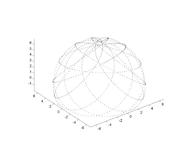
Figure 1. $\scriptstyle(\alpha;\Re\lambda,\Im\lambda;N;J_{1},J_{2},J_{3},x_{1},x_{2},x_{3})=(3.345;0,0.02;1000;2.34,6.4,8,1.219,-0.78,6.77)$

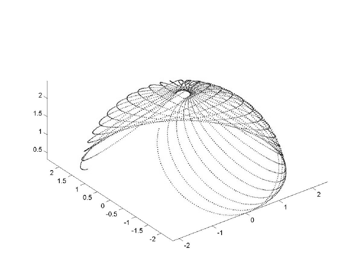
Figure 2. $\scriptstyle(\alpha;\Re\lambda,\Im\lambda;N;J_{1},J_{2},J_{3},x_{1},x_{2},x_{3})=(1;500,5000;4000;3.4,-4.6,-6.2,-2.19,0.89,0.77)$

6. Concluding remarks

We have constructed the 1- and 2-point Bäcklund transformations for the symmetric Lagrange top following the approach of [13]. The application of the constructed maps as exact numerical integrators of the continuous flows is considered. As shown in Section 2 the Lagrange top has the same linear algebraic Poisson structure that belongs to the $sl(2)$ Gaudin magnet. This allowed us to choose the same ansatz for the matrix $M(u)$ (5.1.4) that has been used in [8].

Notice that we had the following algebraic situation, as in Gaudin models: a Lax matrix (5.1.2) which satisfies a linear $r$-matrix algebra (2.0.5) requires a $M$ matrix which comes from a quadratic $r$-matrix algebra (5.1.5). Recall that in the Toda lattice [13] and in the DST model [12] both $L$ and $M$ are derived from the same quadratic $r$-matrix algebra (5.1.5). This fact shall show up in the construction of the quantum analogue of these Bäcklund transformations. Indeed an interesting problem is the quantization of the constructed maps, namely the problem of Baxter $\mathbb{Q}$-operators for the symmetric Lagrange top. Actually this problem leads to the study of product formulae for Heun functions. This work is in progress and the results will be reported in a separate paper.

References

- [1] V.I. Arnold, Mathematical methods of classical mechanics, 2nd edition, Springer (1989).
- [2] M. Audin, Spinning tops, Cambridge University Press (1996).
- [3] L. Gavrilov, Generalized Jacobians of spectral curves and completely integrable systems, Math. Z. 230 (1999), no. 3, 487–508.
- [4] L. Gavrilov, A. Zhivkov, The complex geometry of the Lagrange top, Enseign. Math. (2) 44 (1998), no. 1-2, 133–170.
- [5] M. Gaudin, Diagonalisation d’une classe d’ hamiltoniens de spin, J. de Physique 37 (1976) 1087–1098.
- [6] A.I. Bobenko and Yu. B. Suris, Discrete time Lagrangian mechanics on Lie groups, with an application to the Lagrange top, Commun. Math. Phys. 204 (1999) 147–188.
- [7] M. Gaudin, La fonction d’ onde de Bethe, Masson, Parigi (1983).
- [8] A.N.W. Hone, V.B. Kuznetsov and O. Ragnisco, Bäcklund transformations for the Gaudin magnet, Journal of Physics A 34 (2001), 2477–2490.
- [9] E. Inönü and E.P. Wigner, On the contraction of groups ant their representations, Proc. Natl Acad. Sci. USA 39 510–24.
- [10] V.B. Kuznetsov, Separation of variables for the type periodic Toda lattice, J. Phys. A: Math. Gen. 30 (1997), 2127–2138.
- [11] V.B. Kuznetsov, F.W. Nijhoff and E.K. Sklyanin, Separation of variables for the Ruijsenaars system, Commun. Math. Phys. 189 (1997), 855–877.
- [12] V.B. Kuznetsov, M. Salerno and E.K. Sklyanin, Quantum Bäcklund transformation for DST dimer model, J. Phys. A: Math. Gen. 33 (2000) 171–189
- [13] V.B. Kuznetsov and E.K. Sklyanin, On Bäcklund transformations for many-body systems, J. Phys. A: Math. Gen. 31 (1998) 2241–2251.
- [14] V.B. Kuznetsov and P. Vanhaecke, Bäcklund transformations for finite-dimensional integrable systems: a geometric approach, Journal of Geometry and Physics 44 (2002), 1–40.
- [15] E.K. Sklyanin, Separation of variables. New trends Progr. Theor. Phys. Suppl. 118 (1995) 35–60.
- [16] Yu. B. Suris, The problem of integrable discretization: hamiltonian approach, Birkhäuser Verlag (2003).