Abstract

The Lagrangian complex-space singularities of the steady Eulerian flow with stream function $\sin x_{1}\cos x_{2}$ are studied by numerical and analytical methods. The Lagrangian singular manifold is analytic. Its minimum distance from the real domain decreases logarithmically at short times and exponentially at large times.

Key words: Lagrangian coordinates, singular manifold.

1 Introduction

Singularities of the solutions of hydrodynamical problems in the complex space domain are important, for example, because they allow us to give an objective definition of the otherwise fuzzy concept of “smallest scale present in a flow”. Specifically, if a flow is analytic in the space variable ${\bm{x}}$ for all ${\bm{x}}$, it can be continued to complex ${\bm{z}}={\bm{x}}+i{\bm{y}}$ locations where it will generally have singularities on some complex set $\Sigma$. The minimum distance $\delta$ of $\Sigma$ to the real domain, called the width of the analyticity strip, defines the smallest scale. Indeed, the modulus of the Fourier transforms of the velocity ${\bm{v}}$ decreases roughly as $e^{-\delta k}$ at high wavenumbers $k$; thus the mesh needed in numerically simulating such a flow, e.g. by spectral methods, has to be significantly less than $\delta$ (Sulem, Sulem and Frisch, 1983; Brachet, Meiron, Orszag, Nickel, Morf and Frisch, 1983). Furthermore, should the flow ever develop a real singularity at a finite real time $t_{\star}$, it must be preceded by complex singularities at a distance $\delta(t)$ which continuously vanishes at $t_{\star}$ (Bardos, Benachour and Zerner, 1976; Benachour, 1976a, b). For incompressible flow actual measurements of $\delta(t)$, using high-resolution spectral simulations, indicate that $\delta(t)$ decreases in time, but in a way much tamer than suggested by the known rigorous estimates. In both two and three dimensions the behavior of $\delta(t)$ at large times may well be exponential, but the best estimates are a decreasing double exponential in two dimensions and finite-time blow-up in three dimensions see Frisch, Matsumoto and Bec (2003) for review.

The standard explanation for this discrepancy is the phenomenon of nonlinear depletion, whereby the flow is found to organize itself into structures which have nearly vanishing nonlinearities (Frisch, 1995; Majda and Bertozzi, 2002). Note that one of the features characterizing depletion can be the degree of velocity-vorticity alignment or ”Beltramization” of the flow.

Up to now singularities in the complex domain were studied in Eulerian coordinates. In the present paper we analyse some aspects related to singular behaviour of flows extended into the complex domain in Lagrangian coordinates. One practical motivation of studying Lagrangian singularities in the complex domain concerns the structure of Eulerian singularities of a passive scalar. Indeed, consider a passive scalar advected by an incompressible flow ${\bm{v}}$, whose density satisfies the continuity equation

$$\partial_{t}\theta({\bm{x}},t)+\nabla\cdot(\theta{\bm{v}})=0,$$ (1)

as long as we can neglect molecular diffusion. Obviously, this can be solved by using Lagrangian coordinates:

$$\theta({\bm{x}},t)=\theta_{0}({\bm{a}}({\bm{x}},t)),$$ (2)

where $\theta_{0}$ is the initial density field and ${\bm{a}}({\bm{x}},t)$ is the inverse of the Lagrangian map ${\bm{x}}({\bm{a}},t)$, the latter satisfying the characteristic equation

$$\dot{\bm{x}}={\bm{v}}({\bm{x}},\,t),\qquad{\bm{x}}({\bm{a}},\,0)={\bm{a}}.$$ (3)

If $\theta_{0}$ is devoid of singularities (entire function), it is clear that the singularities of the Eulerian field, continued to complex locations, $\theta({\bm{z}},t)$, will correspond to those (complex) fluid particles trajectories which have started at $t=0$ at (complex) infinity. Furthermore, it implies that the width of the analyticity strip $\delta(t)$ for $\theta({\bm{x}},t)$ in Eulerian coordinates equals the width of the analyticity strip $\delta_{{\mathrm{L}}}(t)$ of the Lagrangian map ${\bm{x}}({\bm{a}},t)$ for the time reversed flow. In Section 4 we will use this correspondence to define the smallest scale of the passive scalar field $\theta({\bm{x}},t)$ at time $t$.

Note that the above argument can be applied to the 2-D vorticity. Assuming infiniteness of Eulerian vorticity at complex Eulerian singularities (Frisch, Matsumoto and Bec, 2003; Matsumoto, Bec and Frisch, 2003) it implies that the Eulerian singularities of solutions of the 2-D Euler equation starting from entire initial data come from the complex infinity. Therefore, especially for the 2-D flows, some understanding of complex singularities in Lagrangian coordinates, even for a very simple flow, can shed light on the nature of Eulerian complex singularities.

S. Orszag (2003) pointed out that the phenomenon of depletion is intrinsically Eulerian and has no Lagrangian counterpart. Thus, it is expected that Lagrangian singularities are stronger - or at least closer to the real domain - than Eulerian ones. An extreme form of depletion is to work with a Beltrami flow given by a steady solution of the incompressible Euler equation such as the ABC flow in three dimensions or the two-dimensional cellular flow with stream function

$$\psi(x_{1},x_{2})=\sin x_{1}\cos x_{2}$$ (4)

and velocity

$$v_{1}=-\sin x_{1}\sin x_{2},\quad v_{2}=-\cos x_{1}\cos x_{2}.$$ (5)

The latter is much simpler, because the Lagrangian map can be obtained explicitly in terms of elliptic functions (Dombre, Frisch, Greene, Hénon, Mehr and Soward, 1986, Appendix A). Moreover, it represents a special case ($A=1$, $B=1$, and $C=0$) of the ABC flow, obtained by applying a transformation of coordinates of the type used in Dombre, Frisch, Greene, Hénon, Mehr and Soward (1986, Appendix A) and reducing the nontrivial dynamics to two dimensions. Our goal in this paper will be to obtain for this flow the complex singularities in Lagrangian coordinates.

The Lagrangian velocity is defined just by the change of variables, that is, as ${\bm{v}}_{{}_{\rm L}}({\bm{a}},t)\equiv{\bm{v}}({\bm{x}}({\bm{a}},t))$ where ${\bm{x}}({\bm{a}},t)$ is the solution of (3) with the velocity given by (5). Of course, such flow being steady, completely lacks Eulerian singularities (except at complex infinity). However, as we shall see, it develops real Lagrangian singularities in infinite time.

The outline of the paper is as follows. In Section 2, we explicitly construct the singular set, the explicit construction of the Lagrangian map being relegated to Appendix A. In Section 3 the Lagrangian velocity, its Fourier transform and $\delta(t)$ are determined numerically. Section 4 is devoted to the short-time and long-time asymptotics.

2 Analytic structure of the singular manifold

We consider the cellular flow on $\mathbb{T}^{2}\equiv[0,2\pi]\times[0,2\pi]$ defined by (4) and (5). Because of the symmetries of this flow the full periodicity domain can be decomposed into four cells, Fig. 1 (a). For convenience, in Fig. 1 (b), we represent the cell $[0,\pi]\times[-\pi/2,\pi/2]$.

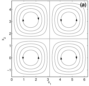
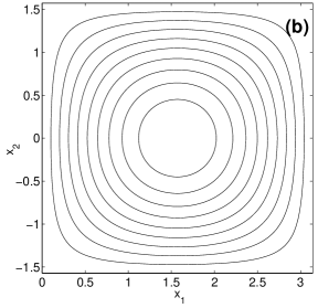
Figure 1: Streamlines for the flow defined by (4) in the (a) flow box, (b) in the basic cell.

The Lagrangian map ${\bm{x}}({\bm{a}},t)$ is the solution of

$$\left\{\begin{array}[]{ll}\dot{x}_{1}=-\sin\ x_{1}\sin\ x_{2};\\ \dot{x}_{2}=-\cos\ x_{1}\cos\ x_{2},\end{array}\right.$$ (6)

with the initial conditions

$$\left\{\begin{array}[]{ll}x_{1}({\bm{a}},\,0)=a_{1};\\ x_{2}({\bm{a}},\,0)=a_{2}.\end{array}\right.$$ (7)

When fluid particles start at complex locations they will stay in the complex domain. We then denote the complexified Lagrangian position by ${\bm{c}}={\bm{a}}+i{\bm{b}}$ and the complexified Eulerian position by ${\bm{z}}={\bm{x}}+i{\bm{y}}$. The complex Lagrangian stream function is $\xi({\bm{c}},t)\equiv\psi({\bm{z}}({\bm{c}},t))$ and the complex Lagrangian velocity is ${\bm{v}}_{{}_{\rm L}}({\bm{c}},t)\equiv{\bm{v}}({\bm{z}}({\bm{c}},t))$.

Since the Eulerian velocity ${\bm{v}}$ is an entire function of ${\bm{z}}$ , the Lagrangian velocity can become singular only where the Lagrangian map becomes singular; furthermore it is easily shown that the only way ${\bm{z}}({\bm{c}},t)$ can become singular, for a finite real $t$ and a complex ${\bm{c}}$, is by going to (complex) infinity.

The explicit solution to (6) is given in the Appendix in terms of elliptic functions. Its form implies the existence of singularities, associated to certain poles of suitable elliptic functions. This is however not the simplest way to actually construct the singular set $\Sigma(t)$, a time-dependent complex manifold of complex dimension one, that is which can be parametrized in terms of one complex parameter. For the construction it is simpler to observe (i) that the value of the complex stream function $\xi$ does not change along fluid particle trajectories and (ii) that the stream function, being the product of $w_{1}\equiv\sin z_{1}$ and $w_{2}\equiv\cos z_{2}$, the only way ${\bm{z}}$ can run to infinity while conserving the stream function is to have either $w_{1}\to\infty$ and $w_{2}\to 0$ or conversely.

In terms of the $w_{1}$ and $w_{2}$ variables, the equations for fluid particle trajectories can be rewritten as

$$\left\{\begin{array}[]{ll}\dot{w}_{1}=-w_{1}\sqrt{1-w_{1}^{2}}\sqrt{1-w_{2}^{2}}\\ \dot{w}_{2}=w_{2}\sqrt{1-w_{2}^{2}}\sqrt{1-w_{1}^{2}}\end{array}\right.$$ (8)

with now complex initial conditions

$$w_{1}(0)=\sin c_{1},\qquad w_{2}(0)=\cos c_{2},$$ (9)

corresponding to the initial conditions (7).

Obviously, the product $\xi=w_{1}w_{2}$ is an integral of motion: this expresses just that for steady flow particles move along streamlines. One can take advantage of this integral of motion to rewrite (8) as a single equation in terms for example of the variable $u\equiv w_{1}/\xi$, as

$$\dot{u}=-i\sqrt{1-u^{2}}\sqrt{1-\xi^{2}u^{2}},\qquad u(0)=u_{0}=(1/\xi)\sin c_{1}.$$ (10)

This equation allows to express the time variable $t$ in terms of the initial and current values of $u$ by an elliptical integral:

$$it=-\int_{u_{0}}^{u(t)}\frac{ds}{\sqrt{(1-s^{2})(1-\xi^{2}s^{2})}}.$$ (11)

We turn now to the determination of the singularities, that is those initial complex locations ${\bm{c}}^{\star}=(c_{1}^{\star},c_{2}^{\star})$ which go to infinity at time $t$. Because of the symmetries of the flow we can, without loss of generality, assume that when ${\bm{z}}\to\infty$ at time $t$, we have $w_{2}\to\infty$ and $w_{1}\to 0$ and hence $u(t)=0$. It follows then from (10) that the singular values of $u_{0}$ are such that

$$it=-\int_{u_{0}}^{0}\frac{ds}{\sqrt{(1-s^{2})(1-\xi^{2}s^{2})}}.$$ (12)

The inverse of the elliptical integral is the elliptic ${\rm sn}$ function (Abramovitz and Stegun, 1965). Thus $u_{0}$ can be expressed as an elliptic function. Since, by (10), $w_{1}(0)=\xi u_{0}$, we obtain

$$w_{1}(0)=\xi\,\mathrm{sn}(it,\xi),\qquad w_{2}(0)=\mathrm{ns}(it,\xi),$$ (13)

where ${\rm ns}\equiv 1/{\rm sn}$. Alternatively, since the ${\rm sn}$ and ${\rm ns}$ functions of imaginary arguments can be expressed in terms of the ${\rm sc}$ function, defined as $\mathrm{sc}\equiv\mathrm{sn}/\mathrm{cn}$, and its reciprocal ${\rm cs}$, we have

$$w_{1}(0)=i\xi\,\mathrm{sc}(t,\sqrt{1-\xi^{2}}),\qquad w_{2}(0)=-i\,\mathrm{cs}(t,\sqrt{1-\xi^{2}}).$$ (14)

By (9), we can express the singular Lagrangian locations at time $t$ as

$$c^{\star}_{1}=\arcsin\left[i\xi\mathrm{sc}(t,\sqrt{1-\xi^{2}})\right],\qquad c^{\star}_{2}=\arccos\left[i\mathrm{cs}(t,\sqrt{1-\xi^{2}})\right].$$ (15)

This constitutes the parametric representation of the singular manifold $\Sigma(t)$, the parameter being the complex stream function $\xi$. Obviously, the functions appearing in this representation are multivalued. More precisely, the singular manifold has infinitely many sheets.

It is well known that elliptic functions are real for real values of the parameters. Therefore, $\Sigma(t)$ will have a non-trivial part “above” the hyperbolic stagnation points, namely the four corners in Fig. 1(b). By symmetry, it is enough to consider one of them. We take $(a_{1},a_{2})=(0,\pi/2)$ and easily obtain the following parametric representation of the singular locations having this stagnation point as real part:

$$b^{\star}_{1}=\mathrm{arcsinh}\left[\xi\mathrm{sc}(t,\sqrt{1-\xi^{2}})\right],\qquad b^{\star}_{2}=\mathrm{arcsinh}\left[-\mathrm{cs}(t,\sqrt{1-\xi^{2}})\right].$$ (16)

Using the parametrization (16) in Fig. 2 (a) we have represented the curve obtained as intersection of the singular manifold with the set of points with real coordinates fixed at $(x_{1},x_{2})=(0,\pi/2)$ , that is the trace of the singular manifold on the pure imaginary plane lying above the corresponding stagnation point. Here ”trace on” is used with its mathematical meaning of ”intersection with”.

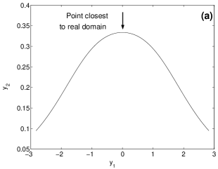
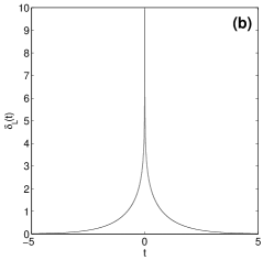
Figure 2: (a) The cut of the singular manifold on the imaginary $(y_{1},y_{2})$-plane is represented. The point closest to the origin lies on the $y_{2}$-axis. (b) Here the value of the closest distance from singular manifold to the real domain, $\delta(t)$, is represented for both positive and negative times.

The width of the Lagrangian analyticity strip $\delta_{\mathrm{L}}(t)$ is obtained by finding the point(s) on the singular manifold closest to the real domain. It seems likely that these points will be located over the points where the flow exhibits a special structure. Indeed, expanding (15) locally in its Taylor series confirms that the points closest to the real domain lie above the hyperbolic stagnation points. The upper left and lower right stagnation points have $b_{1}^{\star}=0$, while the upper right and lower left stagnation points have $b_{2}^{\star}=0$. The distance from the real domain is easily shown to be given by

$$\delta_{\mathrm{L}}(t)=\left|\mathrm{arcsinh}\left(\frac{1}{\sinh t}\right)\right|.$$ (17)

Fig. 2 (b) is a plot of $\delta_{\mathrm{L}}(t)$ showing both positive and negative times.

As we have mentioned in the introduction, $\delta_{\mathrm{L}}(t)$ of the time reversed flow gives the width of the analyticity strip in Eulerian coordinates for a passive scalar satisfying (1) with the same velocity field (5). Indeed, singularities for the passive scalar correspond to (complex) fluid particles which are mapped back to infinity in time $t$. Note that the symmetry of the cellular flow used here implies that $\delta_{\mathrm{L}}(t)$ is an even function of time so that $\delta_{\mathrm{L}}(t)$ of the original flow coincides with the Eulerian $\delta(t)$ for the passive scalar field.

3 Numerical integration in Lagrangian coordinates

In this section we obtain the width $\delta_{\mathrm{L}}(t)$ of the Lagrangian analyticity strip by numerically calculating the Fourier transform of the velocity in Lagrangian coordinates and then applying the method of tracing complex singularities (Sulem, Sulem and Frisch, 1983) to relate the Fourier transform to $\delta_{\mathrm{L}}(t)$. Our method is implemented for the steady cellular flow given by (4) but can in principle be applied to any steady solution of the Euler equation in both two and three dimensions.

We need to calculate the Lagrangian Fourier coefficients, which are here obtained as follows. First, we calculate the Lagrangian map ${\bm{x}}({\bm{a}},t)$ by solving the characteristic equations (6) with a fourth order Runge-Kutta method for $N^{2}$ initial conditions ${\bm{a}}=((2\pi/N)l,\,(2\pi/N)m)\,\,(l,\,m=0,1,\ldots,N-1)$, which form a regular square grid in the Lagrangian marker space. We obtain then the Lagrangian velocity field by just changing variables:

$${\bm{v}}_{\mathrm{L}}({\bm{a}},t)\equiv{\bm{v}}({\bm{x}}({\bm{a}},\ t),\ t),$$ (18)

where ${\bm{v}}({\bm{x}})$ is given by (5). The Lagrangian velocity Fourier coefficients are given by

$$\hat{{\bm{v}}}_{\mathrm{L}}({\bm{k}},\ t)=\frac{1}{N^{2}}\sum_{{\bm{a}}}{\bm{v}}_{\mathrm{L}}({\bm{a}},t)\,e^{-i{\bm{k}}\cdot{\bm{a}}}.$$ (19)

For measuring the width $\delta_{\mathrm{L}}$, it is convenient to define the shell-summed amplitude $A^{({\bm{v}}_{\mathrm{L}})}_{k}$ of $\hat{{\bm{v}}}_{\mathrm{L}}({\bm{k}})$ as

$$A^{({\bm{v}}_{\mathrm{L}})}_{k}=\sum_{k\leq|{\bm{k}}|<k+1}|\hat{{\bm{v}}}_{{\mathrm{L}}}({\bm{k}})|.$$ (20)

The Lagrangian width $\delta_{\mathrm{L}}$ is then obtained by fitting the shell-summed amplitude to an exponential with an algebraic prefactor:

$$A^{({\bm{v}}_{\mathrm{L}})}_{k}\propto k^{-\alpha}\exp(-\delta_{\mathrm{L}}k).$$ (21)

We first discuss how to obtain the width $\delta_{\mathrm{L}}(t)$ at short times when it is very large (since it is infinite at $t=0$). Obtaining $\delta_{\mathrm{L}}(t)$ with a double-precision calculation is not feasible because the Fourier amplitudes $A^{({\bm{v}}_{\mathrm{L}})}_{k}$ fall off too quickly as a function of the wavenumber and thus get lost in the roundoff noise. So we need to solve the equation (6) with higher precision. In practice we divide the time interval $10^{-12}\leq t\leq t$ into four parts: (i) $10^{-12}\leq t<10^{-9}$, (ii) $10^{-9}\leq t<10^{-6}$, (iii)$10^{-6}\leq t<10^{-3}$, (iv) $10^{-3}\leq t<1$. For each part, we use different time step $\Delta t$ and precision: (i) $\Delta t=10^{-12}$ and 48-digit precision, (ii) $\Delta t=10^{-9}$ and 36-digit precision, (iii) $\Delta t=10^{-6}$ and 24-digit precision, (iv) $\Delta t=10^{-3}$ and 15-digit (double) precision. These precisions, for each $\Delta t$, are the best we can handle with the fourth-order Runge-Kutta scheme. Note that in Frisch, Matsumoto and Bec (2003) a 90-digit spectral calculation was used for obtaining the short-time behavior of $\delta(t)$ in Eulerian coordinates for 2-D Euler flow with non-trivial Eulerian dynamics; in the present case, the accuracy of the shell-summed amplitudes $A^{({\bm{v}}_{\mathrm{L}})}_{k}$ is constrained by the accuracy of the time integration scheme of (6). Also we encounter the difficulty that a long-time integration causes serious accumulation of error in vorticity, which eventually breaks the conservation of vorticity (in 2-D vorticity should be conserved along each fluid particle trajectory). That is the reason why we split the time interval $10^{-12}<t<1$ into four parts and use different $\Delta t$ for each part to avoid this accumulation. Figure 3 shows the shell-summed amplitude $A^{({\bm{v}}_{\mathrm{L}})}_{k}$ and the width of the Lagrangian analyticity strip $\delta_{\mathrm{L}}(t)$ at short times $10^{-12}\leq t\leq 1$. As seen in Fig. 3 (a), the number of points in $A^{({\bm{v}}_{\mathrm{L}})}_{k}$ to be fitted is small. We checked that, for several measured $\delta_{\mathrm{L}}(t)$’s shown in Fig. 3 (b), a calculation with smaller $\Delta t$ and higher precision for the same instance gives the same value of $\delta_{\mathrm{L}}(t)$. In this sense, we believe the measured $\delta_{\mathrm{L}}(t)$ is reliable in spite of the very limited data points. From Fig. 3 (b), a clean logarithmic decay of $\delta_{\mathrm{L}}(t)$ is observed for more than 10 decades.

Figure 3: (a) Shell-summed amplitudes of the Lagrangian velocity $A^{({\bm{v}}_{\mathrm{L}})}_{k}$ for four different short times calculated with the number of grid points $32^{2}$ and $64^{2}$. (b) Log-linear plot of the width of the Lagrangian analyticity strip $\delta_{\mathrm{L}}(t)$ measured as the logarithmic decrement of $A^{({\bm{v}}_{\mathrm{L}})}_{k}$ at short times $10^{-12}\leq t\leq 1$.

Now we turn to the numerical determination of the long-time behavior of the width of the Lagrangian analyticity strip. The calculation is straightforward: the characteristic equation (6) is solved with standard double precision using a time step $\Delta t=10^{-3}$. The number of grid points is $4096^{2}$. Figure 4 shows $A^{({\bm{v}}_{\mathrm{L}})}_{k}$ and $\delta_{\mathrm{L}}(t)$ at long times, $0<t\leq 5$. The temporal decrease of $\delta_{\mathrm{L}}(t)$ is exponential in this regime.

This indicates that exponentially small-scale structure is generated in the Lagrangian coordinates by this steady flow. For seeing this, we first show in Fig. 5 the deformation of the initially regular grid caused by the flow. As seen in Fig. 5, the Eulerian field is squeezed around the hyperbolic stagnation points along the contracting direction. We then plot contours of the modulus of the corresponding displacement $|{\bm{x}}({\bm{a}},t)-{\bm{a}}|$ in the Lagrangian coordinates for various instances in Fig. 6. Here we can clearly see that the small-scale structures centered at hyperbolic stagnation points are generated in the Lagrangian coordinates. The exponential decrease of $\delta_{L}(t)$ corresponds to the exponential decrease of the width of the structure in the Lagrangian coordinates centered at the hyperbolic stagnation points.

Figure 4: (a) Shell-summed amplitudes of the Lagrangian velocity $A^{({\bm{v}}_{\mathrm{L}})}_{k}$ for 10 different instances ($t=0.5,1.0,\ldots,5.0$) calculated with the number of grid points $4096^{2}$. (b) Linear-log plot of the width of the Lagrangian analyticity strip $\delta_{\mathrm{L}}(t)$ measured as the logarithmic decrement of $A^{({\bm{v}}_{\mathrm{L}})}_{k}$ at long times $t\leq 5$.

Figure 5: (a) Regular grids in the Eulerian coordinates $(x_{1},\,x_{2})$ at time $t=0$. (b) Advected regular grids by the steady flow at time $t=1.6$, which indicate the Lagrangian map ${\bm{x}}({\bm{a}},t)$ in the Eulerian coordinates. (c) Advected regular grids at time $t=2.4$.

Figure 6: (a) Contours of the modulus of the displacement $|{\bm{x}}({\bm{a}},t)-{\bm{a}}|$ at time $t=1.6$ in the Lagrangian coordinates $(a_{1},\,a_{2})$. Contour levels are $\pi/15,\,2\pi/15,\ldots$. (b) Same as (a) but for $t=2.4$. (c) Same as (a) but for $t=3.2$.

4 Short-time and long-time behavior

The parametric representation (15) for the singular manifold at arbitrary times is somewhat cumbersome. At short times we can use suitable expansions of the trigonometric and elliptic functions (Abramovitz and Stegun, 1965) and obtain to leading order

$$c_{1}^{\star}\backsimeq\mathrm{arcsin}(i\xi t),\qquad c_{2}^{\star}\backsimeq\frac{\pi}{2}+i\,\ln\left(\frac{2}{t}\right),$$ (22)

from which it follows readily that the width of the analyticity strip is

$$\delta_{\mathrm{L}}(t)\backsimeq\ln\frac{2}{t},\qquad t\to 0.$$ (23)

Hence the Lagrangian $\delta_{\mathrm{L}}(t)$ follows a logarithmic law at short time.

We now observe that a short-time logarithmic law for the Eulerian $\delta(t)$ has been obtained by Frisch, Matsumoto and Bec (2003) (see also Matsumoto, Bec and Frisch (2003)) for 2-D flow with a finite number of initial Fourier harmonics. In the present case the Eulerian dynamics are trivial since the flow is time-independent. We believe that a logarithmic law for the short-time behavior of the Lagrangian $\delta_{\mathrm{L}}(t)$ is quite general for steady solutions of the Euler equation with a finite number of harmonics in any dimension $d\geq 2$. Roughly, the argument is as follows. Let $n$ be the degree of the highest-order Fourier harmonic; the velocity at complex locations a large distance $y$ from the real domain grows as $e^{ny}$. Singularities in Lagrangian coordinates at time $t$ correspond to fluid particles which emanated initially from infinity or, equivalently, which are mapped to infinity in a time $t$ under the reversed flow. The latter also grows as $e^{ny}$ at large $y$. A fluid particle located initially within a distance $\delta_{\mathrm{L}}\gg 1$ of the real domain and having an imaginary component of the velocity $O\left(e^{ny}\right)$ will escape to infinity in a time approximately given by

$$t=\int_{\delta_{\mathrm{L}}}^{\infty}e^{-ny}dy=\frac{1}{n}e^{-n\delta_{\mathrm{L}}}.$$ (24)

It follows that

$$\delta_{\mathrm{L}}(t)\backsimeq\frac{1}{n}\ln\frac{1}{nt}.$$ (25)

It is not clear whether this law for the Lagrangian $\delta_{\mathrm{L}}$ will carry over to flow having non-trivial Eulerian dynamics.

We now turn to the long-time behavior. In Eulerian coordinates for non-trivial dynamics the best proven lower bound for $\delta(t)$ is a decreasing double exponential (see Frisch, Matsumoto and Bec (2003) and references therein). But numerical simulations usually give a simple exponential decrease (Sulem, Sulem and Frisch, 1983; Frisch, Matsumoto and Bec, 2003). The Lagrangian $\delta_{\mathrm{L}}$ for the steady cellular flow considered here is given by (17), which has an obvious expansion at large $t$

$$\delta_{\mathrm{L}}(t)\backsimeq 2e^{-t},\qquad t\to\infty,$$ (26)

which agrees with the numerical simulations of Section 3. Note that the nearest singularities are located “above” the hyperbolic stagnation points of the flow (5).

As we have remarked in Section 1 $\delta_{\mathrm{L}}(t)$ allows us to give an objective definition of the smallest scale for the passive scalar advected by the flow (5). According to formula (26) this scale decreases exponentially in time which, as we have noted in Section 3, reflects the squeezing of the flow around the hyperbolic stagnation points. The exponential temporal rate of deformation of passive scalar structures transversal to the streamlines can be explained by dimensional reasoning.

We note that the period of motion of a particle along a trajectory with the stream function $\Psi({\bm{a}})$ is given by $4K(\sqrt{1-\Psi^{2}({\bm{a}})})$ (see Appendix A, formula (A.4) and (Lawden, 1989)) changing from $2\pi$ in the centre of the cell to infinity at the boundaries. Obviously, for a passive scalar field which is not constant along the streamlines, such as for example $\theta(x_{1},x_{2})=\cos x_{1}\sin x_{2}$, the most intensive mixing will be observed near the hyperbolic stagnation points. Let us consider the flow near the stagnation point $(0,\pi/2)$ at the point ${\bm{a}}=(a_{1},\pi/2-a_{2})$. The displacement of a fluid particle starting at ${\bm{a}}$ becomes significant at the time $t\sim K(\sqrt{1-\Psi^{2}({\bm{a}})})$. Since $\Psi({\bm{a}})$ is small, we use the approximative expression (see (Whittaker and Watson, 1927))

$$K(\sqrt{1-\Psi^{2}({\bm{a}})})\approx\ln\frac{4}{\Psi({\bm{a}})}$$ (27)

and obtain

$$a_{1}a_{2}\sim e^{-t}.$$ (28)

Hence the smallest spatial scale for the passive scalar will decrease exponentially in time.

In this paper, it is found that hyperbolic stagnation points can be a key in the analysis the width of the Lagrangian analyticity strip of the steady solution (4) to the 2-D Euler equation. Currently we are investigating the Lagrangian $\delta_{\mathrm{L}}(t)$ of the 3-D steady solutions (the ABC flows and more general Beltrami flows (Majda and Bertozzi, 2002)) of the 3-D Euler equations. Since such flows can be chaotic, an interesting question is which stretching — caused by the chaos or the hyperbolic stagnation points — dominates. A preliminary result indicates that the nearest singularities are again above the hyperbolic stagnation points at large times. The details of the study of the 3-D steady flows will be reported elsewhere. It is also of interest to point out that for kinematic dynamos in three-dimensional steady flows, the fastest growth of the magnetic field is frequently observed near hyperbolic stagnation points (Soward, 1994) despite the presence of the chaotic stretching.

A question for further study remains whether the behaviour of the Lagrangian $\delta_{\mathrm{L}}(t)$ does exhibit some structural stability with respect to hyperbolic stagnation points.

Acknowledgments. We are grateful to J. Bec and U. Frisch for useful discussions. Computational resources were provided by the Yukawa Institute (Kyoto). This research was supported by the European Union under contract HPRN-CT-2000-00162 and by the Indo-French Centre for the Promotion of Advanced Research (IFCPAR 2404-2). WP would like to thank U. Frisch, A. Degenhard and Yu. G. Kondratiev for their support and help. TM was supported by the Japanese Ministry of Education Grant-in-Aid for Young Scientists [(B), 15740237, 2003] and received also partial support from the French Ministry of Education.

Appendix

Appendix A Explicit construction of the Lagrangian map

The system of ordinary differential equations (6) can be solved by a simple adaptation of what is done for an integrable case of the ABC flow in (Dombre, Frisch, Greene, Hénon, Mehr and Soward, 1986, Appendix A). For completeness we give the full derivation, which is quite elementary.

Taking the derivative of (6) with respect to time we obtain a system of two decoupled differential equations

$$\left\{\begin{array}[]{ll}2\ddot{x}_{1}=\sin 2x_{1}\\ 2\ddot{x}_{2}=-\sin 2x_{2},\end{array}\right.$$ (A.1)

satisfying the initial conditions (7) and

$$\left\{\begin{array}[]{ll}\dot{x}_{1}({\bm{a}},\,0)=-\sin a_{1}\sin a_{2}\\ \dot{x}_{2}({\bm{a}},\,0)=-\cos a_{1}\cos a_{2}.\end{array}\right.$$ (A.2)

Eq. (A.1) is obviously the same as a set of pendulum equations describing nonlinear oscillations around the origin for the $x_{2}$-variable and around $\pi/2$ for the $x_{1}$-variable. Let us just consider the $x_{2}$-variable. The equation has the first integral

$$\frac{1}{2}\dot{x}_{2}^{2}-\frac{1}{4}\cos 2x_{2}=\frac{1}{4}-\frac{1}{2}\sin^{2}a_{1}\cos^{2}a_{2}=\frac{1}{4}\left(1-2\Psi^{2}(\mathbf{a})\right),$$ (A.3)

which expresses the conservation of energy. From this equation we obtain by standard integration (Lawden, 1989)

$$\sin x_{2}(\mathbf{a},t)=\sqrt{1-\Psi^{2}(\mathbf{a})}\mathrm{sn}\left(t+\int_{0}^{a_{2}}\frac{d\tilde{x}}{\sqrt{(1-\Psi^{2}(\mathbf{a}))-\sin^{2}\tilde{x}}},\sqrt{1-\Psi^{2}(\mathbf{a})}\right)$$ (A.4)

Obviously, since the poles of the $\mathrm{sn}$ function do not lie on the real axis (Lawden, 1989; Abramovitz and Stegun, 1965), solutions of (6) are periodic and nonsingular for real initial conditions. The only possibility for an orbit to come across a pole and thereby to go to infinity is to start at a suitable complex location.

References

- Abramovitz and Stegun (1965) Abramovitz, M. and Stegun, I.A., Handbook of Mathematical Functions, Dover Publications (1965).
- Bailey (1995) Bailey, D.H., “A fortran-90 based multiprecision system”, RNR Technical Report RNR-94-013 (1995). See also http://crd.lbl.gov/dhbailey/
- Bardos, Benachour and Zerner (1976) Bardos, C., Benachour, S. and Zerner, M., “Analyticité des solutions périodiques de l’équation d’Euler en deux dimensions” , C. R. Acad. Sc. Paris 282 A, 995-998 (1976).
- Benachour (1976a) Benachour, S., “Analyticité des solutions de l’équation d’Euler en trois dimensions”, C. R. Acad. Sc. Paris 283 A, 107-110 (1976).
- Benachour (1976b) Benachour, S., “Analyticité des solutions des équations d’Euler”, Arch. Rat. Mech. Anal. 71, 271–299 (1976).
- Brachet, Meiron, Orszag, Nickel, Morf and Frisch (1983) Brachet, M.E., Meiron, D. I., Orszag, S.A., Nickel, B.G., Morf, R.H. and Frisch, U., “Small-scale structure of the Taylor-Green vortex”, J. Fluid Mech. 130, 411–452 (1983).
- Dombre, Frisch, Greene, Hénon, Mehr and Soward (1986) Dombre, T., Frisch, U., Greene, J.M., Hénon, M., Mehr, A. and Soward, A.M., “Chaotic Streamlines in the ABC flows”, J. Fluid Mech. 167, 353–391 (1986).
- Frisch (1995) Frisch, U., Turbulence. The legacy of A.N. Kolmogorov, Cambridge Univ. Press (1995).
- Frisch, Matsumoto and Bec (2003) Frisch, U., Matsumoto, T. and Bec, J., “Singularities of Euler flow? Not out of the blue!”, J. Stat. Phys. 113, 761–781 (2003). (nlin.CD/0209059).
- Lawden (1989) Lawden, D.F., Elliptic Functions and Applications, Springer-Verlag (1989).
- Majda and Bertozzi (2002) Majda, A. J. and Bertozzi, A.L., Vorticity and Incompressible Flow, Cambridge University Press (2002).
- Matsumoto, Bec and Frisch (2003) Matsumoto, T., Bec, J. and Frisch, U., “The analytic structure of 2D Euler flow at short times”, Fluid Dyn. Res. in press (2004). (nlin.CD/0310044).
- Ohkitani (2002) Ohkitani, K., “Numerical study of comparison of vorticity and passive vectors in turbulence and inviscid flows”, Phys. Rev. E 65, 046304 (2002).
- Orszag (2003) Orszag, S.A., Private communication to U. Frisch (2003).
- Soward (1994) Soward, A.M., “Fast dynamos”, in Lectures on Solar and Planetary Dynamos, eds. M.R.E. Proctor and A.D. Gilbert, p. 181-217, Cambridge University Press, Cambridge (1994).
- Sulem, Sulem and Frisch (1983) Sulem, C., Sulem, P.L. and Frisch, H., “Tracing complex singularties with spectral methods”, J. Comput. Phys. 50, 138–161 (1983).
- Whittaker and Watson (1927) Whittaker, E. T. and Watson, G. N., A Course of Modern Analysis, Cambridge at the University Press (1927).