Chemical turbulence equivalent to Nikolavskii turbulence

Abstract

We find evidence that a certain class of reaction-diffusion systems can exhibit chemical turbulence equivalent to Nikolaevskii turbulence. The distinctive characteristic of this type of turbulence is that it results from the interaction of weakly stable long-wavelength modes and unstable short-wavelength modes. We indirectly study this class of reaction-diffusion systems by considering an extended complex Ginzburg-Landau (CGL) equation that was previously derived from this class of reaction-diffusion systems. First, we show numerically that the power spectrum of this CGL equation in a particular regime is qualitatively quite similar to that of the Nikolaevskii equation. Then, we demonstrate that the Nikolaevskii equation can in fact be obtained from this CGL equation through a phase reduction procedure applied in the neighborhood of a codimension-two Turing–Benjamin-Feir point.

The onset of spatiotemporal chaos is an important subject in the study of dissipative systems K84 ; Cro ; Boh ; Man . Several yeas ago, a new mechanism causing the onset of spatiotemporal chaos was discovered by Tribelsky et al. Tri-discover for the Nikolaevskii equation,

$$\partial_{t}u=-\partial_{r}^{2}[\epsilon-(1+\partial_{r}^{2})^{2}]u-(\partial_{r}u)^{2}.$$ (1)

This equation was originally proposed to describe the propagation of longitudinal seismic waves in viscoelastic media Nik . Its uniform steady state $u=0$ is unstable with respect to finite-wavelength perturbations when the small parameter $\epsilon$ is positive. However, this instability does not lead to spatially periodic steady states, because the equation possesses a Goldstone mode, due to its invariance under transformations of the form $u\rightarrow u+const.$, and the corresponding weakly stable long-wavelength modes interact with the unstable short-wavelength modes. As a consequence, spatially periodic steady states do not occur, and instead spatiotemporal chaos occurs supercritically. This chaos is called ‘Nikolaevskii turbulence’. Its properties have been investigated by several authors Tri1 ; Kli ; Tri2 ; Xi-Amp ; Mat ; Tor ; Fuj-Amp .

Although it is conjectured that spatiotemporal chaos exhibiting a similar onset appears in various systems, experimentally only one such phenomenon has been observed to this time, complex electrohydrodynamic convection (also called ‘soft-mode turbulence’), discovered in homeotropically aligned nematic liquidcrystals by Kai et al. Kai ; Ros ; Tri-liq_cry ; Nag ; Tam . Similar onset has also been studied numerically in systems exhibiting Rayleigh-B$\acute{{\rm e}}$nard convection under free-free boundary conditions by Xi et al. Xi-RB , and the possibility for the existence of this type of turbulence in reaction-diffusion systems has been investigated by Fujisaka and Yamada Fuj and independently by Tanaka and Kuramoto Dan .

In this letter, we present further evidence for the ubiquity of the type of spatiotemporal chaos described above. We find evidence that the chaos exhibited in a particular regime by a complex Ginzburg-Landau equation with nonlocal coupling Dan , called a nonlocal CGL equation, is equivalent to Nikolaevskii turbulence. This suggests that a certain class of oscillatory reaction-diffusion systems can also exhibit this type of chaos, because the nonlocal CGL is a reduced form of this class of reaction-diffusion systems K95 ; Dan . These reaction-diffusion systems are such that the chemical component constituing local oscillators are only weakly diffusive, while there is an extra diffusive component introducing an effectively nonlocal coupling between the oscillators. Such a situation, in which the coupling between the local oscillators is mediated by a diffusive substance, has been observed in some systems studied experimentally: biological populations, such as cellular slime molds bio2 and oscillating yeast cells under glycolysis bio4 , catalytic CO oxidation on metal surfaces Kim , and the Belousov-Zhabotinsky reaction exhibited by a system dispersed in a water-in-oil aerosol OT microemulsion Van . Because these systems possess such coupling, it is conjectured that under certain circumstances they could exhibit spatiotemporal chaos in the same class as Nikolaevskii turbulence.

Our starting point is the following nonlocal CGL equation with complex amplitude $A$:

$$\partial_{t}A = A-(1+ic_{2})|A|^{2}A+(\delta_{1}+i\delta_{2})\nabla^{2}A$$ (2)

$$+K(1+ic_{1})\int\!\!d{\bm{r}}^{\prime}G({\bm{r}}-{\bm{r}}^{\prime})[A({\bm{r}}^{\prime})-A({\bm{r}})].$$

Here $G$ is a coupling function, and $c_{1}$, $c_{2}$, $\delta_{1}$, $\delta_{2}$ and $K$ are real parameters. In a previous paper Dan , this equation was derived as a generic reduced form of the class of reaction-diffusion systems discussed above. A simple example that belongs to this class is the following set of equations, describing a hypothetical extended Brusselator:

$$\partial_{t}X = a-(b+1)X+X^{2}Y+D\nabla^{2}X+kc_{X}S,$$ (3)

$$\partial_{t}Y = bX-X^{2}Y+D\nabla^{2}Y+kc_{Y}S,$$ (4)

$$\tau\partial_{t}S = -a-S+\nabla^{2}S+X,$$ (5)

where the field variables $X$ and $Y$ represent limit-cycle oscillators existing immediately above the Hopf bifurcation, and the additional chemical component $S$ introduces an effective nonlocal coupling between these oscillators. The strength and anisotropy of this coupling are represented by the parameters $k$ and $c_{X,Y}$ respectively. The Hopf bifurcation parameter $\mu$ is written in terms of the parameters $a$ and $b$ as $\mu\equiv(b-b_{c})/b_{c}$, where $b_{c}=1+a^{2}$. The coefficient $D$ is the diffusion constant for $X$ and $Y$, and the quantity $\tau$ is the time constant of $S$. When these couplings are as weak as the oscillation, i.e., when $\mu\sim O(D)\sim O(k)$, this system can be reduced to Eq. (2).

Equation (2) is invariant under transformations of the form $A\rightarrow Ae^{ic}$, with real constant $c$, which implies that a uniform mode is neutrally stable. This is a result of the spontaneous breaking of time translational symmetry corresponding to the Hopf bifurcation in the original reaction-diffusion systems. Also, the uniform oscillating solution of Eq. (2) possesses a Turing instability Tur in a certain parameter region, as shown in Fig. 1, in contrast to the ordinary diffusive complex Ginzburg-Landau equation, which possesses only a Benjamin-Feir instability. Thus, Eq. (2) in this parameter region is characterized by weakly stable long-wavelength modes and unstable short-wavelength modes, like Eq. (1). Therefore, it has been hypothesized that Eq. (2) exhibits spatiotemporal chaos similar to Nikolaevskii turbulence Dan . We confirm this hypothesis in the following.

Figure 1: Parameter space $(K,Kc_{1})$ in the neighborhood of a codimension-two Turing–Benjamin-Feir point. The uniform ocsillating solution of the nonlocal CGL is stable in domain $S$, possesses the Turing instablility above the curve $l_{T}$ and the Benjamin-Feir instablility above the line $l_{BF}$. The parameter values are $c2=1$, $\delta_{1}=0.3$, $\delta_{2}=0$, and $G(r)=\rho/2\ e^{-\rho|r|}$, with $\rho=1+0.905i$. The inset plots the stability eigenvalue as a function of the perturbation wavenumber for the uniform ocsillating solution at the point $(K,Kc_{1})=(0.05,-0.4345)$, indicated by the cross. The largest eigenvalue is nearly equal to $0.0005$ at the Turing wavenumber, which is approximately $0.6$. This dispersion curve is qualitatively the same as that of the Nikolaevskii equation.

For simplicity, we fix the parameter values as $c_{2}=1$ and $\delta_{2}=0$ and consider only the case of one spatial dimension. In this case, the coupling function $G(r)$ is given by $G(r)=\rho/2\ e^{-\rho|r|}$, with $\rho=1+i\eta$ and $1>\eta\geq 0$, where the form of $G(r)$ is derived from the original reaction-diffusion systems Dan . However, the following analysis is applicable also in higher-dimensional situations, in which $G$ takes other forms.

A typical spatiotemporal pattern exhibited by Eq. (2) in the slightly Turing-unstable regime close to the Benjamin-Feir criticality is shown in Fig. 2, where we see long-wavelength modulation of the Turing pattern. The corresponding spatial power spectrum is displayed in Fig. 3. This spectrum is found to have characteristic peaks at the Turing wavenumber and its harmonics. This feature is also seen in the spectrum of Nikolaevskii turbulence, shown in the inset of Fig. 3. This suggests that in the regime we consider, the spatiotemporal chaos exhibited by Eq. (2) is in the same class as Nikolaevskii turbulence. In the following, we show that, in fact, Eq. (1) can be obtained from Eq. (2) by means of a phase reduction technique K84 .

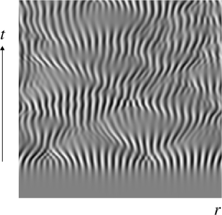
Figure 2: Gray level plots of $\Psi(r,t)\equiv\partial_{r}\arg[A(r,t)]$, which corresponds to $\partial_{r}u$ of the Nikolaevskii equation Eq. (1). The width of the longitudinal stripes corresponds to the Turing wavelength. The parameter values are indicated by the cross in Fig. 1. The configuration displayed here represents the result obtained after evolution from an initial configuration (which is the uniform ocsillating solution with a slight perturbation) over a time interval of length $10^{5}$ in a periodic one-dimensional system consisting of $2^{10}$ spatial points separated by a distance of $0.3$. For the numerical scheme, we used a pseudo-spectral method with an explicit fourth-order Runge-Kutta scheme of time step $0.01$.

Figure 3: Spatial power spectrum of $\Psi(r,t)$. This spectrum was calculated using a system size ($0.3\times 2^{12}$ spatial points) larger than that of Fig. 2 and averaged over a long time, excluding an initial transient of length $5\times 10^{4}$. The inset displays typical spatial power spectra obtained from the Nikolaevskii equation, Eq. (1), with $\epsilon=0.02$ (bottom) and the well-known Kuramoto-Sivashinsky equation (top), for the sake of comparison. The peaks are characteristic of Nikolaevskii turbulence. The spectrum of the nonlocal CGL exhibits similar peaks at the Turing wavenumber and its harmonics.

In the phase reduction, the diffusion term and the nonlocal-coupling term of Eq. (2) are treated as perturbations. Using Floquet theory, we can calculate the operator ${\bm{Z}}(\phi)$ that projects the perturbation onto the limit cycle $A^{0}(\phi)=e^{-i\phi}$ of the unperturbed system: ${\bm{Z}}(\phi)=(\cos\phi-\sin\phi,-\sin\phi-\cos\phi)$. Hence, the phase dynamics of Eq. (2) obey

$$\partial_{t}\phi = 1+\delta_{1}\partial_{r}^{2}\phi-\delta_{1}(\partial_{r}\phi)^{2}$$ (6)

$$+\int\!\!dr^{\prime}\Gamma(\phi-\phi^{\prime},r-r^{\prime}),$$

$$\Gamma(\phi,r) = \frac{K|\alpha|}{2}e^{-|r|}[\sin(\phi-\eta\ |r|+\arg\alpha)$$ (7)

$$\mbox{\hskip 42.67912pt}-\sin(-\eta\ |r|+\arg\alpha)],$$

where $\phi(r,t)$ and $\phi(r^{\prime},t)$ are abbreviated as $\phi$ and $\phi^{\prime}$, respectively, and $\alpha=[-c_{1}-1+i(1-c_{1})]\rho$. In the integrand $\Gamma(\phi-\phi^{\prime},r-r^{\prime})$ there is a dependence on the quantity $\phi-(\phi^{\prime}+\eta|r-r^{\prime}|)$; i.e., the time evolution of the phase at $r$ depends not on the difference between the phases at $r$ and $r^{\prime}$ but on the difference between the phase at $r$ and the phase at $r^{\prime}$ plus the quantity $\eta|r-r^{\prime}|$. This might seem paradoxical for the following reason. If the spatial interactions are weak, then $\partial_{t}\phi\simeq 1$, and hence $\phi(r^{\prime},t)+\eta|r-r^{\prime}|\simeq\phi(r^{\prime},t+t_{0})$ with $t_{0}=\eta|r-r^{\prime}|$. Thus the phase at $r$ interacts with the future phase $\phi(r^{\prime},t+t_{0})$, where $t_{0}\geq 0$ because $\eta\geq 0$. To solve this paradox, note that the original reaction-diffusion fields oscillate roughly as $\cos\Phi$ with $\Phi=\omega_{0}t-\mu\phi$, where the Hopf frequency $\omega_{0}$ is a finite positive value, and the Hopf bifurcation parameter $\mu$ is an extremely small positive value Dan . Thus, $\Phi(r,t)$ interacts with $\Phi(r^{\prime},t-t_{1})$ with $t_{1}=\mu t_{0}/\omega_{0}$ if we ignore terms of $O(\mu^{2})$. Hence the field at $r$ interacts with the past field at $r^{\prime}$, as $t_{1}\geq 0$. In this sense, $\eta$ producing the imaginary part in the coupling function $G$ in Eq. (2) causes the phase coupling to be implicitly delayed, with the delay proportional to the distance between interacting oscillators.

Now we rescale the phase equation derived above. First, we introduce a variable $\psi$ defined as $\psi\equiv\phi-t$. The evolution equation for $\psi$ is the same as that of $\phi$, except for the absence of the term $1$ on the right-hand side. Instead of Eq. (6), we refer to the equation for $\psi$ as the phase equation in the following. In the long-wavelength limit, where the validity of the phase description is ensured because the amplitude-like modes can be safely ignored, the phase equation can be expanded in a power series in $\partial_{r}^{2}$, owing to the symmetry of the system with respect to reflection through $r=0$: $\partial_{t}\psi=(\lambda_{2}\partial_{r}^{2}+\lambda_{4}\partial_{r}^{4}+\lambda_{6}\partial_{r}^{6}+\cdots)\psi+N$. Here $N$ represents the nonlinear terms, and $\lambda_{n}$ are constants derived from $c_{1}$, $\delta_{1}$, $K$ and $\eta$ . We consider the Turing-unstable regime close to the Benjamin-Feir criticality, where $\lambda_{2},\lambda_{4},\lambda_{6}>0$, $\lambda_{2}\sim O(\nu^{2})$, $\lambda_{4}\sim O(\nu)$, and $\lambda_{6}\sim O(1)$, with the scaling parameter $\nu=+0$, and $4\lambda_{2}\lambda_{6}=(1-\epsilon)\lambda_{4}^{2}$ with a positive constant $\epsilon\ll 1$. Under these conditions, the higher-derivative linear terms, $\partial_{r}^{n}\psi$ with $n\geq 8$, are much smaller than the other linear terms and can be ignored because the characteristic spatial scale of $\psi$ is $\sim O(\nu^{-1/2})$. Furthermore, because $\psi$ itself has a characteristic small magnitude depending on $\nu$, it is reasonable to assume that the largest nonlinear term in $N$ is $\gamma(\partial_{r}\psi)^{2}$, where $\gamma$ is a constant derived from $c_{1}$, $\delta_{1}$, $K$ and $\eta$ . In fact, when we rescale $r$, $t$ and $\psi$ as $r\rightarrow\tilde{r}=\sqrt{\frac{\lambda_{4}}{2\lambda_{6}}}r$, $t\rightarrow\tilde{t}=\frac{\lambda_{4}^{3}}{8\lambda_{6}^{2}}t$ and $\psi\rightarrow\tilde{\psi}=\frac{-4\gamma\lambda_{6}}{\lambda_{4}^{2}}\psi$, we can obtain the following scale-free equation from the phase equation:

$$\partial_{\tilde{t}}\tilde{\psi}=-\partial_{\tilde{r}}^{2}[\epsilon-(1+\partial_{\tilde{r}}^{2})^{2}]\tilde{\psi}-(\partial_{\tilde{r}}\tilde{\psi})^{2}.$$ (8)

This is identical to Eq. (1). Here, note that $\tilde{\psi}$ satisfies the scaling relation

$$\psi(r,t) = \nu^{2}\tilde{\psi}(\nu^{1/2}r,\nu^{3}t).$$ (9)

This spatiotemporal scaling of the phase is completely different from the scaling relation in the case that the Kuramoto-Sivashinsky equation is derived, $\psi(r,t)=\xi\tilde{\psi}(\xi^{1/2}r,\xi^{2}t)$, where $\xi$ is a parameter that represents the Benjamin-Feir criticality.

The above parameter conditions resulting in the derivation of Eq. (8) can be written in terms of the parameters of Eq. (2) as follows. Using $\zeta\equiv\arctan\eta$, where $\pi/4>\zeta\geq 0$ because $1>\eta\geq 0$, Eq. (8) is derived from Eq. (2) under the following conditions, with a sufficiently small positive constant $\nu$ when $\zeta\neq 0,\pi/8$:

$$K(1+ic_{1}) = \Upsilon\exp[i(4\zeta+3\pi/4-\nu)],$$ (10)

where

$$\Upsilon = \frac{\delta_{1}}{\sqrt{2}(\cos\zeta)^{2}}\left[\sin(2\zeta-\nu)+\frac{(1-\epsilon)(\sin\nu)^{2}}{4\sin(2\zeta+\nu)}\right]^{-1}.$$ (11)

Here, the parameter $\epsilon$ is the same as that in Eq. (8), and the critical value of $\Upsilon$ is $\Upsilon_{c}=\delta_{1}[\sqrt{2}(\cos\zeta)^{2}\sin(2\zeta)]^{-1}$.

In order to observe the same spatiotemporal chaos as that of Nikolaevskii turbulence in our reaction-diffusion systems, we can analytically tune these parameters to satisfy the above conditions. In particular, the time constant $\tau$ of the additional chemical $S$ (e.g., see Eq. (5)) should be nonzero, because $\zeta=[\arctan(\omega_{0}\tau)]/2\neq 0$, where $\omega_{0}$ is the Hopf frequency Dan . This reflects the importance of the imaginary part in the coupling function $G$ of Eq. (2), i.e., the implicit delay of the phase coupling discussed above. This contrasts with the situation found in previous studies of similar reaction-diffusion systems, in which the limit $\tau\rightarrow 0$ was taken and $S$ was eliminated adiabatically K95 ; tau0-0 ; tau0-1 ; tau0-2 ; tau0-3 . In addition to the condition $\tau\neq 0$, we should also have $\tau\neq 1/\omega_{0}$, because $\zeta\neq\pi/8$. This implies that the charcteristic time of the field $S$ is not comparable to that of the local oscillator, $(X,Y)$.

In conclusion, we have found evidence that the nonlocal CGL and the corresponding class of reaction-diffusion systems in a certain regime exhibit turbulence that is equivalent to Nikolaevskii turbulence. This result supports the conjecture of the ubiquitous nature of spatiotemporal chaos caused by the interaction between weakly stable long-wavelength modes and unstable short-wavelength modes. We have confirmed through numerical calculation that these chaotic states are structurally stable for the nonlocal CGL not just at the codimension-two Turing–Benjamin-Feir point but also in a finite neighborhood around it, at points where the CGL equation does not reduce exactly to the Nikolaevskii equation. Furthermore, we believe that similar spatiotemporal chaos would be found even if the phase-shift invariance were sligthly broken in the reaction-diffusion systems; i.e, this chaos should persist even if the Goldstone mode were lost. This conjecture is based on the observation that soft-mode turbulence exists even if one applies a small magnetic field that slightly breaks the arbitrariness of the azimuthal angle of directors bent through a Freedericksz transition in homeotropically aligned liquidcrystals Huh . Finally, we note that the phase equation derived from the nonlocal CGL is a useful model for studying quantitative features of Nikolaevskii turbulence that has not yet been investigated sufficiently. Because this phase equation covers the transition region between Nikolaevskii turbulence and the well-known Kuramoto-Sivashinsky turbulence, it can be used not only for comparing these two types of turbulence but also for exploring the transition between them. This should lead to deeper understanding of Nikolaevskii turbulence and also a broader class of turbulence caused by interactions among modes with vastly different length scales.

The author is grateful to Y. Kuramoto for useful discussions, to S. Kai, Y. Hidaka, and K. Tamura for valuable discussions on their experimental results, to H. Fujisaka for interesting comments, and to H. Nakao for carefully reading the manuscript.

References

- (1) Y. Kuramoto, Chemical Oscillation, Waves, and Turbulence (Springer, New York, 1984); (Dover Edition, 2003).
- (2) M. C. Cross and P. C. Hohenberg, Rev. Mod. Phys. 65, 851 (1993).
- (3) T. Bohr et al., Dynamical Systems Approach to Turbulence (Cambridge University Press, Cambridge, 1998).
- (4) P. Manneville, Dissipative Structures and Weak Turbulence (Academic Press, Boston, 1990).
- (5) M. I. Tribelsky and K. Tsuboi, Phys. Rev. Lett. 76, 1631 (1996); M. I. Tribelsky and M. G. Velarde, Phys. Rev. E 54, 4973 (1996).
- (6) V. N. Nikolaevskii, in Recent Advances in Engineering Science, edited by S. L. Koh and C. G. Speciale, Lecture Notes in Engineering Vol.39 (Springer-Verlag, Berlin, 1989), p. 210.
- (7) M. I. Tribel’skii, Phys. Usp. 40, 159 (1997).
- (8) I. L. Kliakhandler and B. A. Malomed, Phys. Lett. A 231, 191 (1997).
- (9) M. I. Tribel’skii, Macromol. Symp. 160, 225 (2000).
- (10) H.-W. Xi, R. Toral, J. D. Gunton, and M. I. Tribelsky, Phys. Rev. E 62, R17 (2000).
- (11) P. C. Matthews and S. M. Cox, Phys. Rev. E 62, R1473 (2000).
- (12) R. Toral, G. Xiong, J D Gunton, and H. Xi, J. Phys. A: Math. Gen. 36, 1323 (2003).
- (13) H. Fujisaka, T. Honkawa, and T. Yamada, Prog. Theor. Phys. 109, 911 (2003).
- (14) S. Kai, K. Hayashi, and Y. Hidaka, J. Phys. Chem. 100, 19 007 (1996).
- (15) A. G. Rossberg, A. Hertrich, L. Kramer, and W. Pesch, Phys. Rev. Lett. 76, 4729 (1996).
- (16) M. I. Tribelsky, Phys. Rev. E 59, 3729 (1999).
- (17) T. Nagaya and H. Orihara, J. Phys. Soc. Japan 69, 3146 (2000).
- (18) K. Tamura, Y. Yusuf, Y. Hidaka, and S. Kai, J. Phys. Soc. Japan 70, 2805 (2001).
- (19) H.-W. Xi, X.-J. Li, and J. D. Gunton, Phys. Rev. Lett. 78, 1046 (1997).
- (20) H. Fujisaka and T. Yamada, Prog. Theor. Phys. 106, 315 (2001).
- (21) D. Tanaka and Y. Kuramoto Phys. Rev. E 68, 026219 (2003).
- (22) Y. Kuramoto, Prog. Theor. Phys. 94, 321 (1995).
- (23) A. T. Winfree, The Geometry of Biological Time (Springer, New York 1980).
- (24) S. Dano, P. G. Sorensen, and F. Hynne, Nature 402, 320 (1999).
- (25) M. Kim, M. Bertram, M. Pollmann, A. V. Oertzen, A. S. Mikhailov, H. H. Rotermund, and G. Ertl, Science 292, 1357 (2001).
- (26) V. K. Vanag and I. R. Epstein, Phys. Rev. Lett. 87, 228301 (2001); Science 294, 835 (2001); Phys. Rev. Lett. 88, 088303 (2002); Phys. Rev. Lett. 90, 098301 (2003).
- (27) A. M. Turing, Philos. Trans. R. Soc. London B 237, 37 (1952).
- (28) Y. Kuramoto, H. Nakao, and D. Battogtokh, Physica A 288, 244 (2000).
- (29) H. Nakao, T. Mishiro, and M. Yamada, Int. J. Bifurcation Chaos 11, 1483 (2001).
- (30) D. Battogtokh and Y. Kuramoto, Phys. Rev. E. 61, 3227 (2000).
- (31) Y. Kuramoto and S. Shima, Prog. Theor. Phys. Suppl. 150, 115 (2003).
- (32) J.-H. Huh, Y. Hidaka, and S. Kai, 67, 1948 (1998); J.-H. Huh, Y. Hidaka, and S. Kai, J. Phys. Soc. Japan 68, 1567 (1999).