Anisotropic fluctuations in turbulent sheared flows

Abstract

An experimental analysis of small-scales anisotropic turbulent fluctuations has been performed in two different flows. We analyzed anisotropic properties of an homogeneous shear flows and of a turbulent boundary layer by means of two cross-wire probes to obtain multi-point multi-component measurements. Data are analyzed at changing inter-probe separation without the use of Taylor hypothesis. The results are consistent with the “exponent-only” scenario for universality, i.e. all experimental data can be fit by fixing the same set of anisotropic scaling exponents at changing only prefactors, for different shear intensities and boundary conditions.

I Introduction

Statistical theory of turbulence is often focused on homogeneous and isotropic flows fri95 . Experimentally, however, we know that isotropy holds approximately, with different degrees of justification, depending on the geometry of the boundaries and on the driving mechanism. Therefore, a realistic description of turbulence cannot ignore anisotropic and non-homogeneous effects, especially in regions close to the boundaries, and/or at scales close to the integral scale, $L_{0}$, where the injection mechanism can strongly affect velocity fluctuations. The interest of quantifying anisotropic and non-homogeneous effects is also linked to the important issue of “recovery of isotropy”, i.e. the problem of “small-scales universality”. Surprisingly enough, recent experimental and numerical works gar98 ; she00 ; she02a ; pum96 ; bif01a ; bif01 have detected the survival of anisotropic turbulent fluctuations till to the Kolmogorov scale, $\eta$. These findings have stimulated a lot of further experimental, numerical and theoretical work focused to develop proper analytical tools ara99b and to extend the available experimental/numerical data sets gar98 ; she00 ; she02a ; pum96 ; ara99 ; bif01a ; bif01 ; ara98 ; kur00 ; kur00a . Many progresses have been done. For example, the so-called puzzle of “persistence of anisotropies” in small-scales –high Reynolds numbers– sheared flows, has been recently understood as the effect of the presence of strong anomalous anisotropic fluctuations bif01 ; bif02 . The attention is mainly focused on correlation functions based on gradients (to probe Reynolds number dependencies) or to the projections on isotropic/anisotropic sectors of multi-points velocity correlation functions, $S^{\{\alpha\}}(\mbox{\boldmath$r$}_{1},\dots,\mbox{\boldmath$r$}_{n})\equiv\left\langle v_{\alpha_{1}}(\mbox{\boldmath$r$}_{1})\dots v_{\alpha_{n}}(\mbox{\boldmath$r$}_{n})\right\rangle$, where we use $\{\alpha\}$ as a shorthand notation for the ensemble of indexes $\alpha_{1},\dots,\alpha_{n}$ . When all spatial separation, $\mbox{\boldmath$r$}_{1}\dots\mbox{\boldmath$r$}_{n}$, are in the inertial range, $\eta\ll|\mbox{\boldmath$r$}_{i}-\mbox{\boldmath$r$}_{j}|\sim r\ll L_{0}$, one expects the existence of power laws behavior under a uniform space dilation: $S^{\{\alpha\}}(\lambda\mbox{\boldmath$r$}_{1},\dots,\lambda\mbox{\boldmath$r$}_{n})=\lambda^{\xi(n)}S^{\{\alpha\}}(\mbox{\boldmath$r$}_{1},\dots,\mbox{\boldmath$r$}_{n})$. Most of the recent works in anisotropic turbulence concentrated on determining the values of the exponent, $\xi(n)$, as a function of the order of the correlation function, $n$, and of its anisotropic properties. Indeed, an important step forward has been done by realizing that different projections of the multi-point correlation functions on different irreducible representation of the group of rotation, SO(3), possess different scaling properties. The idea is to decompose any correlation function in a complete basis of eigenfunctions with defined properties under rotations. Each eigenfunction identifies a specific anisotropic sector with total angular momentum, $j$, and its projection, $m$, on a given axis. It is believed that the scaling properties of the projections on different sectors possess different scaling exponents, $\xi_{j}(n)$.

Exponents for the fully isotropic sectors are labeled by $j=0$ while more and more anisotropic fluctuations are measured by higher and higher values of $j$ ara99b ; ara98 .

The higher-than-expected presence of small-scales anisotropic fluctuations raises questions about their universal or non-universal origins. In other words, one is interested to control if all flows posses the same, or similar, anisotropic small-scales fluctuations independently on their large-scale behavior. Of course, full universality cannot be expected, one is tempted to believed to a “exponent-only” scenario, i.e. only the scaling exponents, $\xi_{j}(n)$, pertaining to each different anisotropic sector, are universal, while the overall correlation functions intensities are not. This hypothesis is inspired by both theoretical reasons ara99b ; dec and similarities with what observed for isotropic fluctuations arneodo .

Up to now, there are a few experimental and numerical data sets where universality of anisotropic fluctuations has been probed. In particular, as of today, we have some detailed experimental investigation of anisotropic small-scale fluctuations in homogeneous shear flows she00 ; she02a , in atmospheric boundary layer ara98 ; kur00 ; kur00a and in windtunnel data wandervater . From the numerical side, only a few Direct Numerical Simulations (DNS) in highly anisotropic flows have been performed with the aim to explicitly test the small-scales properties of anisotropic fluctuations ara99 ; Mazzitelli ; bif01a ; bif03a ; bif02 . The situation is still moot. On the experimental side, because of the difficulty to have multi-point multi-components velocity measurements one can access only the $j=2$ sector. On the other hand, DNS can properly disentangle fluctuations of all sectors, but due to limitations in the Reynolds numbers, only results in the $j=4$ and $j=6$ sectors have been obtained with some accuracy. The $j=2$ sector in the numerical works bif01a ; bif03a was not measurable due to strong finite Reynolds effects. Results from different experiments, with different geometries and different large scale structures, are in fairly good agreement concerning the $j=2$ sector up to moment $n=6$. Putting together all results of numerics and experiments one recovers a scenario for anisotropic fluctuations consistent (not in contradiction) with the “exponent-only” picture of universality. Still, more tests in both experiments and numerics are needed.

The aim of this paper is to present a new systematic assessment of anisotropic fluctuations in sheared flows at changing both the experimental set-up and the shear intensity. In particular, we have measured small-scales turbulent properties in a homogeneous shear flow (HS) and in a turbulent boundary layer (TBL). One of the novelties here presented consists in the using of measurements from two cross-wire probes at changing their separation, i.e. we do not need to use Taylor hypothesis of frozen turbulence in order to extract information at different scales. This kind of multi-points multi-components measurements are necessary in order to disentangle contributions from isotropic and anisotropic fluctuations and among different kind of anisotropic fluctuations.
Our results support the “exponent-only” scenario. We found good qualitative, and quantitative, agreement of the anisotropic scaling exponents in both HS and TBL flows. Moreover our results are in agreement with the previously measured values in different experiments with different Reynolds numbers and different shear intensities.
The paper is organized as follows. In sec. II we present the details of the two experimental apparatus including some typical large-scale measurements to validate the laboratory set-up. In sec. III we present the scaling properties for both HS and TBL flows. Conclusions follow in sec. IV.

II Experimental set-up

The data we are going to discuss concern two different experiments, both conducted in the $1.30\nobreak\mbox{$\;$m}\times 0.90\nobreak\mbox{$\;$m}$ test section of a 7 m long open return wind tunnel. The first data-set has been obtained in a nominally homogeneous shear flow (HS), characterized by a constant velocity gradient. The second one refers to measurements performed in the logarithmic region of a zero-pressure gradient turbulent boundary layer (TBL).

II.1 Homogeneous shear flow

Figure 1: Homogeneous shear flow: mean velocity profile as a function of the non-dimensional coordinate in the mean gradient direction, $y/h$. In the inset, the normalized streamwise turbulent intensity $u_{\rm rms}$. Velocities are normalized in terms of the centerline velocity, $U_{c}=10.2\,\nobreak\mbox{$\;$m\,s${}^{-1}$}$, while the test section height is $h=0.9\,\nobreak\mbox{$\;$m}$.

$u_{\rm rms}$	$v_{\rm rms}$	$\rho_{uv}$	$\epsilon$	$\ell_{\rm T}$	$\eta$	$Re_{\lambda}$	$S^{*}$
( m s-1)	( m s-1)		($\;{\rm m}^{2}\,{\rm s}^{-3}$)	( mm)	( mm)
0.43	0.31	-0.29	0.6	53	0.28	170	4.9

Table 1: Basic parameters for the homogeneous shear flow. Symbols are defined as follows: The rms fluctuation intensity in the streamwise direction is $u_{\rm rms}={\langle(u-U)^{2}\rangle}^{1/2}$, and analogous definitions apply for $v_{\rm rms}$ and $w_{\rm rms}$. $\rho_{uv}=\langle uv\rangle/(u_{\rm rms}\,v_{\rm rms})$ is the correlation coefficient, $\epsilon$ is the energy dissipation rate evaluated in terms of the one-dimensional spectrum $E_{11}(\kappa_{1})$: $15\,\nu\int\kappa_{1}^{2}E_{11}(\kappa_{1})\,d\kappa_{1}\,$. $\ell_{\rm T}$ is the transverse integral length scale, $\int\langle\,u(x,y,z)\,u(x,y,z+r_{z})\,\rangle\,dr_{z}/u_{\rm rms}^{2}$ and $\eta=(\nu^{3}/\epsilon)^{1/4}$ is the Kolmogorov scale. The Taylor-Reynolds number is $Re_{\lambda}=\lambda u_{\rm rms}/\nu$, where the Taylor scale follows from $\sqrt{15\nu u_{\rm rms}^{2}/\epsilon}$ and the shear parameter is $S^{*}=\sqrt{Su_{\rm rms}^{2}/\epsilon}$.

The set-up of the homogeneous shear flow is based on the original idea proposed in Tavoularis . The mean shear is generated with a device consisting of a series of $15$ adjacent small channels, equipped with screens of different solidity to produce suitable pressure drops. The channels are followed by flow straighteners in such a way that sufficiently downstream the mean velocity profile $U(y)$ is linear in the core region. The data shown in figure 1 correspond to a measurement approximately $4.8\nobreak\mbox{$\;$m}$ downstream of the apparatus, where the flow is already well developed. Concerning fluctuations, the deviations from the ideal constant profile of the streamwise turbulence intensity $u_{\rm rms}(y)={\,\langle\,(u-U)^{2}\,\rangle\,^{\frac{1}{2}}}$ are comparable with what observed in similar set-up gar98 . In particular, in the central part of the test section where the data discussed below have been acquired, they are of the order of $7\,\%$. The dimensionless shear rate $S^{*}\simeq 5$ (table 1), is a factor two smaller than what achieved in the logarithmic part of the turbulent boundary layer (table 2).

II.2 Boundary layer

The boundary layer develops on the smooth surface of the lower wall of the tunnel, where a nominal zero pressure-gradient is achieved by adjusting the upper wall. The measurements have been performed on the centerline of the test section, $6.0\nobreak\mbox{$\;$m}$ downstream the tripping device at the end of the contraction. With an external velocity $U_{\infty}$ of $11.5\,\rm{m/s}$, the thickness of the boundary layer at this location is approximately $\delta\simeq 40\,\rm{mm}$, while the Reynolds number based on the momentum thickness $Re_{\theta}$ is approximately $6500$, well within the range pertaining to a fully developed turbulent boundary layer. The friction velocity, $u_{\tau}=\sqrt{\tau_{w}/\rho}$ with $\tau_{w}$ the average shear stress at the wall and $\rho$ the constant density, estimated from the mean velocity profile with a Clauser chart, is found to be $u_{\tau}=0.43\nobreak\mbox{$\;$m\,s${}^{-1}$}$, in good agreement ($\pm 8\%$) with a direct measurement by means of a Preston tube. The streamwise mean velocity $U(y)$ and the fluctuation intensity $u_{\rm rms}(y)$ profiles are displayed in Figure 2. Both curves show that the flow complies to the requirements of a fully developed turbulent boundary layer.

Figure 2: Turbulent boundary layer: Mean velocity profile $U^{+}$ vs wall normal distance $y^{+}$ in wall units. The dotted line corresponds to the linear behavior $U^{+}=y^{+}$, while the solid line indicates the log-law: $U^{+}=(1/\kappa)\,{\mbox{ln}}\,y^{+}+B$, with $\kappa=0.41$ and $B=5.1$. The inset shows the streamwise turbulent fluctuation $u^{+}_{\rm rms}$. Wall units are defined in terms of the friction velocity and the kinematic viscosity $\nu$, thus $U^{+}=U/u_{\tau}$, $u^{+}_{\rm rms}=u_{\rm rms}/u_{\tau}$ and $y^{+}\,=\,u_{\tau}\,y/\nu$.

$y^{+}$	$u_{\rm rms}$	$v_{\rm rms}$	$\rho_{uv}$	$\epsilon$	$\ell_{\rm T}$	$\eta$	$Re_{\lambda}$	$S^{*}$
	( m s-1)	( m s-1)		($\;{\rm m}^{2}\,{\rm s}^{-3}$)	( mm)	( mm)
350	0.94	0.45	-0.37	7.1	12.2	0.15	330	12.1
240	1.01	0.47	-0.39	11.	8.6.	0.13	300	12.8
140	1.06	0.48	-0.38	13.7	7.1	0.125	250	14.2
90	1.07	0.46	-0.36	23.	6.6	0.11	230	15.9

Table 2: Basic parameters for the boundary layer. For definitions see caption of table 1.

II.3 Data acquisition

The instrumentation consists essentially of a couple of sub-miniature X-probes, mounted on streamlined supports in order to minimize interference effects, and separated in the transverse direction, see figure 3. The wires are $2.5\,\nobreak\mbox{$\,$ $\mu\,$m}$ in diameter, $0.5\nobreak\mbox{$\;$mm}$ in effective length and in separation, oriented at $\pm 45^{\circ}$ with respect to the streamwise direction. They are operated at an overheat ratio 1.9. Single component sub-miniature probes (diameter $2.5\,\nobreak\mbox{$\,$ $\mu\,$m}$, length to diameter ratio equal to 200 to minimize conduction losses) have also been used to measure the velocity profiles. The signals from the two X-wires are simultaneously digitized at 21  kHz with a 16-bit data-acquisition board, after being low-pass filtered at the Nyquist frequency and suitably amplified to achieve a good signal-to-noise ratio. The frequency response of the hot-wires, measured in the free stream at a reference velocity $U=6\,\nobreak\mbox{$\;$m\,s${}^{-1}$}$, is larger than 15 kHz. In this way, the resolution needed to analyze the small scales behavior down to the Kolmogorov length-scale $\eta$ - typically of the order of $0.1\div 0.2\nobreak\mbox{$\;$mm}\,$ - is guaranteed. The X-wires are calibrated in situ against a Pitot tube. The mapping between the output voltages and the components of the velocity (u,v) is obtained by varying both the reference velocities and the orientation of the probe with respect to the flow (see, e.g., Meneveau ). The calibration was repeated at the end of each set of measurements, to check that no voltage drift had occurred.

As for the length of the signals, they consist typically of $4\div 8\times 10^{6}$ samples, corresponding roughly to $2\times 10^{4}$ eddy turnover times for both flows. Convergence of the statistics has been checked up to the $6^{\rm th}$ moment.

III Results

Scaling properties of anisotropic fluctuations are traditionally addressed through objects that are identically zero in homogeneous isotropic conditions. Typically, the study has been confined to the co-spectra lumley . Recently a new extended set of observables has been proposed in the context of the $\rm SO(3)$ decomposition. The idea is to exploit the expansion of any generic statistical observable in terms of a suitable eigen-basis with a well characterized behavior under rotations she02a ; kur00 . Let us focus, for instance, on the generic element in the space of second order correlation tensors

$$S_{\alpha_{1}\alpha_{2}}({\bf r})\,=\,\langle\,\delta v_{\alpha_{1}}({\bf r})\delta v_{\alpha_{2}}({\bf r})\,\rangle\,,$$ (1)

where $\delta v_{\alpha}({\bf r})$ denotes the $\alpha^{\rm th}$ component of the velocity increment at two points separated by the vector ${\bf r}$, $\delta v_{\alpha}({\bf r})\equiv v_{\alpha}(\mbox{\boldmath$x$}+\mbox{\boldmath$r$})-v_{\alpha}(\mbox{\boldmath$x$})$. The appropriate SO(3) decomposition of (1) reads ara99b :

$$S_{\alpha_{1}\alpha_{2}}({\bf{r}})\,=\,\sum_{j=0}^{\infty}\,\,\,\sum_{m=-j}^{+j}\,\,\,\sum_{q=1}^{p(j)}\,\,\,S_{jmq}^{(2)}({r})\,B^{jmq}_{\alpha_{1}\alpha_{2}}(\hat{\bf{r}})\ .$$

Here the index $j$ denotes a sector, to be understood as a subspace invariant with respect to rotations, $B^{jqm}_{\alpha_{1}\alpha_{2}}$ denote the appropriate basis function ara99b which depend on the unit vector $\hat{\bf{r}}$ and $p(j)$ counts the number of irreducible representations. In particular, $j=0$ labels the isotropic sector, while sectors of increasing anisotropy correspond to higher and higher $j$’s. Information on the dynamics of the system is now captured by the coefficients $S_{jmq}^{(2)}$ which depend only on distance $r$.

The invariance under rotations of the inertial terms of the Navier-Stokes equations suggests that small-scales statistics depend only on the sector under consideration. For Reynolds large enough, scaling laws of the projection are therefore expected in the form

$$S_{jmq}^{(2)}(r)\sim r^{\xi_{j}(2)},$$

where the scaling exponent explicitly depend on the sector, $j$, while the argument $2$ reminds that we are presently dealing with a second order tensor. The machinery can be easily extended to structure functions of any order $n$,

$$S_{{\alpha_{1}}\ldots{\alpha_{n}}}({\bf r})\,=\,\langle\,\delta v_{\alpha_{1}}({\bf r})\ldots\delta v_{\alpha_{n}}({\bf r})\,\rangle\,,$$ (2)

whose projection on the proper SO(3) basis will possess a scaling behavior:

$$S^{\,(n)}_{jmq}(r)\sim r^{\xi_{j}(n)}.$$

In this context, the recovery of isotropy at smaller and smaller scales correspond to the existence of a hierarchy of exponents $\xi_{j=0}(n)<\xi_{j}(n)$ ara99b ; bif01 .

Scaling laws for the anisotropic sectors has been recently addressed by using different DNS databases Mazzitelli ; bif01 ; bif01a . From the experimental point of view, the evaluation of the proper $\rm SO(3)$ components of a given correlation tensor is hampered by the limited information on its spatial dependence. In the latter case, the simplest approach is to make a selection of tensorial components such as to cancel out the isotropic contribution in the expansion (III). For example, the component $S_{12}(\mbox{\boldmath$r$})$ in the direction $\mbox{\boldmath$r$}=(0,0,r_{3})$ vanishes in a purely isotropic ensemble. Still, in principle all anisotropic sectors may influence its behavior. One may follow two possibilities. Either one may extract the whole anisotropic spectrum by making a multi-parameter fit in all sectors ara98 or may assume, as done in the present paper, that at scales small enough the correlation function is dominated by the leading anisotropic contribution she02a ; kur00 . Considering that in the geometrical set-up of our interest the $j=1$ sector is absent by symmetry, one assumes that in the small-scales limit (at high Reynolds numbers) the leading behavior of (III) is given by the $j=2$ sector:

$$S_{\alpha_{1}\alpha_{2}}({\bf{r}})\,\sim\,\sum_{m=-2}^{+2}\,\,\,\sum_{q=1}^{p(2)}\,\,\,S_{2mq}^{(2)}({r})\,B^{2mq}_{\alpha_{1}\alpha_{2}}(\hat{\bf{r}})\ .$$

Clearly, using this procedure, systematic, out-of-control, errors are introduced by neglecting the higher $j$ sectors. Similar consideration can be extended to tensorial correlation functions of any order.

n	separation	Observable
$2$	$r_{1}$	$S_{12}(r_{1})$
$4$	$r_{1}$	$S_{1112}(r_{1})$	$S_{1222}(r_{1})$
$6$	$r_{1}$	$S_{111112}(r_{1})$	$S_{111222}(r_{1})$	$S_{122222}(r_{1})$
$2$	$r_{3}$	$S_{12}(r_{3})$
$4$	$r_{3}$	$S_{1112}(r_{3})$	$S_{1222}(r_{3})$
$6$	$r_{3}$	$S_{111112}(r_{3})$	$S_{111222}(r_{3})$	$S_{122222}(r_{3})$

Table 3: List of observables with null contribution from the $j=0$ and $1$ sectors.

For example, table 3 lists several observables which, according to the previous discussion and the symmetries of the experimental set-up sketched in figure 3, do not present contributions from both sectors $j=0$ and $j=1$. In the table, the suffixes $1$, $2$ and $3$ correspond to direction $x_{1}=x$, $x_{2}=y$ and $x_{3}=z$, respectively. The objects reported in the first three lines depend on the streamwise separation $r_{1}$, they can be evaluated by using a single X-wire probe and Taylor hypothesis. Those on the last three lines depend on the transverse separation $r_{3}$ and can be measured only by using at least two X-wire probes. Hereafter we mainly present results based on the two-probes approach.

Considering the schematic of figure 3, the two points measurements consist in the acquisition of $u$ and $v$ at two points separated in direction $z$ (see caption).

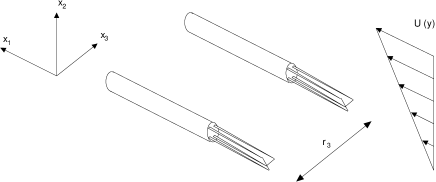
Figure 3: Schematic of the measurement configuration: each of the two X-wires, separated in the transverse direction, $z=x_{3}$, detects two velocity components $u$ and $v$ (in the streamwise, $x=x_{1}$, and in the shear direction $y=x_{2}$, respectively). The separation between the two probes was measured by means of a CCD camera with a high magnification lens and could be changed by means of a precision transverse gear from $0.8\nobreak\mbox{$\;$mm}$ to $70\nobreak\mbox{$\;$mm}$.

On the other hand, for example, the single point measurement of $S_{1112}(r_{1})$ with $u_{1}=u$ and $u_{2}=v$, as a function of time yields

$$S_{1112}(r_{1})\,=\qquad\qquad\qquad\qquad\qquad\qquad\qquad\qquad$$

$$\langle\,\left[\,u(t\,+\,r_{1}/U)\,-\,u(t)\,\right]^{3}\,\left[\,v(t\,+\,r_{1}/U)\,-\,v(t)\,\right]\,\rangle\ .$$ (3)

This approach has been used e.g. in she02a in the context of the homogeneous shear flow and in kur00 at a single location in the atmospheric boundary layer to address the scaling properties of the $j=2$ sector. In kur00a , two single component wires, at fixed separation in the transverse direction $z$, are used in connection with Taylor hypothesis to extract the scaling exponent of the $j=2$ sector while a similar procedure with two X-wires separated in the shear direction $y$ permits to investigate the scaling behavior of the $j=1$ sector.

Purpose of the present work is to by-pass the use of Taylor hypothesis by using the configuration described in the schematic of figure 3. This allows to compute the anisotropic observables depending on $r_{3}$ (table 3) by continuously changing the transverse separation between the two probes.

III.1 The homogeneous shear flow

The global parameters characterizing the homogeneous shear flow are summarized in table 1. In order to allow for the direct comparison of the data for the homogeneous shear flow with those for the boundary layer that are presented in subsection III.2, a common normalization procedure is used. For the homogeneous shear the relevant characteristic velocity is defined as

$$u_{\tau}\,=\,\sqrt{\tau/\rho}$$ (4)

where the total shear stress is given by $\tau=\nu S\,-\,\langle uv\rangle$ where $S=dU/dy$ is the mean shear.

In figure 4, the second order mixed structure function $S_{12}(r_{3})$ is plotted as a function of the transverse separation. In addition to the $r^{2}$ behavior at smaller scales and to the large scale saturation, a power-law at intermediate scales emerges distinctly, allowing us to measure the scaling exponent $\xi_{2}(2)$ with good accuracy. The estimate $\xi_{2}(2)=1.2\,\pm 0.07$ is indicated by the solid line, while the horizontal plateau in the inset, displaying the structure function in compensated form, shows the extension of the scaling region.

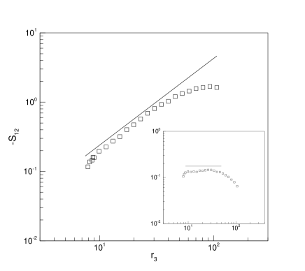
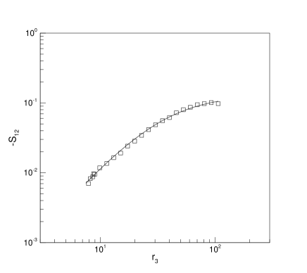
Figure 4: Homogeneous shear flow. Top: Log-log plot of the mixed structure function of second order, $-S_{12}$ plotted as a function of the transverse separation $r_{3}$. All quantities are normalized with respect to the inner scaling defined by $u_{\tau}=\sqrt{\tau/\rho}$ and $\nu/u_{\tau}$. The solid line corresponds to the slope $1.2$. The minimal length scale resolved is of the order of the dissipative scale. In the inset the same data are shown in compensated form, $-S_{12}/{r_{3}}^{1.2}$. Bottom: The same data are fitted by means of the expression given in equation (5), with $A_{2}=0.018$, $B_{2}=0.062$ and $D_{2}=3.27$, solid line.

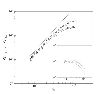
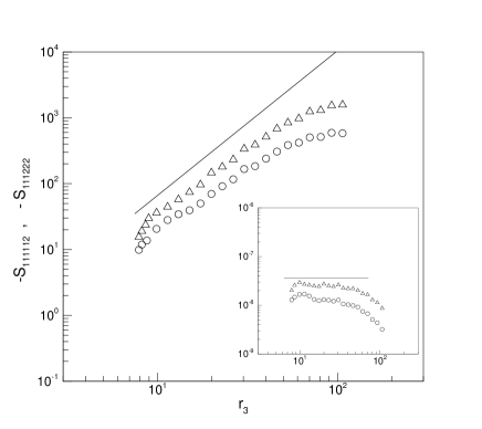
Figure 5: Homogeneous shear flow. Top panel: The purely anisotropic mixed structure functions of order $4$, $S_{1112}$ (triangles) and $S_{1222}$ (circles). The solid line indicates the slope of $1.7$. In the inset the same data are compensated with $r^{1.7}$, same symbols. Bottom plot: Two purely anisotropic mixed structure functions of order $6$, $S_{111112}$ (triangles) and $S_{111222}$ (circles). The solid line indicates the slope of $2.05$. In the inset the same data are compensated with $r^{2.05}$, same symbols.

The same data have also been fitted by means of the expression proposed in kur00 to model the behavior of a generic structure function in the entire range of scales (bottom panel, solid line). In our case, the interpolation function for $S_{12}(r_{3})$ is given by

$$S_{12}(r_{3})\,=\,\frac{A_{2}\,r_{3}^{2}\,\left[\,1\,+\,D_{2}\,\left(\,r_{3}/\ell_{\rm T}\,\right)\,\right]^{-\xi_{2}(2)}}{\left[\,1\,+\,B_{2}\,\left(\,r_{3}/\eta\,\right)^{2}\,\right]^{1-\left[{\xi_{2}(2)}\right]/2}\,}\,.$$ (5)

and describes the superposition of a scaling behavior with coefficient $\xi_{2}(2)$ at intermediate scales, a large-scale saturation and a dissipative closure at small scales. Here, the exponent $\xi_{2}(2)$ is fixed by the direct fit estimated from the compensated plot in the top panel of figure 4, the transverse integral scale $\ell_{\rm T}$ is evaluated according to its definition given in table 1, while $A_{2}$ and $B_{2}$ are the only two fitting constants. The ability of equation (5) to correctly reproduce the experimental data can be appreciated by looking at the excellent agreement between the solid curve and the open symbols in the bottom panel of figure 4. Such an extra fitting procedure, not strictly necessary here, turns out to be useful later in the context of the TBL flow.

Results concerning higher-order statistics of anisotropic fluctuations are reported in figure 5. In the top panel, the two transverse observables of order four, namely $S_{1112}(r_{3})$ and $S_{1222}(r_{3})$ are shown, both in their standard and compensated forms. A best fit yields for the exponent $\xi_{2}(4)$ a value of $1.7\pm 0.1$, indicated by the solid line. The associated error accounts for both the deviation from a pure scaling law and for the slightly different behavior of $S_{1112}(r_{3})$ with respect to $S_{1222}(r_{3})$. The corresponding compensated structure functions of order four are shown in the inset of the top panel. Mixed structure functions of order six are displayed in the bottom panel of figure 5. In particular, with the configuration of figure 3, three transverse observables can be measured, namely $S_{111112}(r_{3})$, $S_{111222}(r_{3})$ and $S_{122222}(r_{3})$. Only the first two, with the best statistical properties, are shown in the figure. Here again, minimal differences in the scaling behavior of these quantities are observed. Typically, lower values of the exponents are achieved for structure functions with largest weight on the vertical velocity component, i.e. for the sixth order $S_{122222}$. The exponents increase with increasing weight of $u$, i.e. for the sixth order moving from $S_{122222}$ through $S_{111222}$ to $S_{111112}$. However, we find that a unique value of $\xi_{2}(6)=2.05\,\pm 0.15$ is able to fit satisfactorily the set of statistics of order six.

The scaling exponents extracted by the present procedure are consistent with the values given in she02a and in kur00 , namely $\xi_{2}(2)=1.05\div 1.22$, $\xi_{2}(4)=1.42\div 1.56$ and $\xi_{2}(6)=1.71\div 2.14$.

III.2 The turbulent boundary layer

To address the effect of the shear intensity and of different boundary conditions, we consider the more complex environment represented by the near-wall region of a fully developed turbulent boundary layer. In this flow configuration two basic difficulties emerge. The first one is associated with the thinness of the region where significant changes of the mean gradient occur which poses severe restrictions on the probe dimensions. The second problem is related to the relatively large fluctuation level in the lower part of the log-region, which may cause troubles with Taylor hypothesis. Concerning the first issue, a boundary layer as thick as possible was realized in a relatively large, yet well-controlled, experimental facility, as described in section II.

Figure 6: Turbulent boundary layer: log-log plot of the mixed structure functions vs transverse separation $r_{3}$ at different wall distances $y^{+}=350$ (triangles), $240$ (diamonds), $140$ (squares), $90$ (circles) and for different orders $n=2,\,4,\,6$. In the top panel we show $-S_{12}$ (second order) where the corresponding solid lines represent the fit (7) keeping fixed $\xi_{2}(2)=1.2$ at varying $A_{2},\,D_{2}$. The inset shows $-S_{12}$ in raw form (open triangles) and after compensation with saturation and viscous contributions (filled triangles) at $y^{+}=350$. The solid line indicates the slope $1.2$. In the middle panel we show $-S_{1112}$ (fourth order), with $\xi_{2}(4)=1.7$ at varying $A_{4},\,D_{4}$. In the inset we show the anisotropic flatness $-S_{1112}/S_{12}^{2}$ at corresponding locations. The solid line indicates the slope $-.65$. In the bottom panel we show $-S_{111112}$ (sixth order) with $\xi_{2}(6)=2.05$ at varying $A_{6},\,D_{6}$.

Moreover, to ensure a sufficient probe resolution, the measurements were limited to the log-region, sufficiently far from the boundary. The second point was instead entirely by-passed by addressing anisotropic observables depending only on the transverse separation $r_{3}$, as already explained for the HS configuration. Also for the boundary layer, the data we discuss are presented in dimensionless form, using the friction velocity

$$u_{\tau}\,=\,\sqrt{\tau_{w}/\rho}\,$$ (6)

as characteristic velocity scale, where $\tau_{w}$ is the average shear stress at the wall (section II). This corresponds directly to the normalization used in subsection III.1, since in the near-wall region the total shear stress $\tau$ is constant in the wall-normal direction. The main issue is connected to the assessment of the anisotropic properties at changing distance from the wall.

In figure 6 we summarize the results for the fully anisotropic transverse structure functions already introduced in the previous section. The three panels show, from top to bottom, the observables of order 2, 4 and 6, respectively, while the different symbols correspond to different distances from the wall, from $y^{+}=350$ down to $y^{+}=90$. As one can see, the scaling properties are not as clear as in the HS case. Independently of the order of the structure function, farther from the wall a distinct scaling range emerges. As the wall is approached, the scaling behavior is less evident and a tendency towards saturation at large scales is observed. Here, in order to extract quantitative results one needs to consider also large scale effects. In particular, we generalized the expression (5) to all orders, for separations much larger than the Kolmogorov scale:

$$S_{\alpha_{1}\ldots\alpha_{n}}(r_{3})\,=\,{A_{n}(y^{+})\,r_{3}^{\xi_{2}(n)}\,\left[\,1\,+\,D_{n}(y^{+})\,\frac{\displaystyle r_{3}}{\displaystyle\ell_{\rm T}}\,\right]^{-\xi_{2}(n)}}\,.$$ (7)

By comparing the fit with the raw data, it is quite clear that the poor scaling closer to the wall is substantially explained in terms of saturation occurring earlier and earlier as the wall is approached. The inset in the top panel describes the fitting procedure and highlights the scaling law by removing the effect of the large scale saturation. The inset of the middle panel shows the anisotropic flatness, $-S_{1122}/S_{12}^{2}$, to highlight the high degree of intermittency showed by anisotropic fluctuations, independently on the distance from the wall. It is important to stress here that the good agreement with the data for all distances is obtained by keeping fixed the scaling exponents $\xi_{2}(n)$ to the value obtained in the HS case for all orders $n$ –only prefactors change at changing the wall distance.

IV Concluding Remarks

In this paper we have performed a systematic analysis of small-scales anisotropic turbulent properties in two different experimental set-up, a homogeneous shear and a turbulent boundary layer. We have used two cross-wires probes in order to extract the leading anisotropic fluctuations of two-point correlation functions in the homogeneous directions without the needing of Taylor hypothesis. We have analyzed structure functions up to order $n=6$ finding a good agreement of the anisotropic exponents between the two experimental set-up and at changing the distance from the wall in the turbulent boundary layer. We could compare the anisotropic properties by changing the normalized shear intensity, $S^{*}$, by a factor 2 and more.
The cleanest data are obtained for the homogeneous shear flow where a fit of the power law behavior allowed for a direct measurement of the anisotropic properties. In the turbulent boundary layer, we had to take into account also large scale saturation effects, especially close to the wall, in order to obtain a global fit of the structure functions behavior for all value of $y^{+}$. Our results support the “exponent-only” scenario of universality also in the anisotropic sector. In other word, we have been able to fit all experimental data by keeping fixed the scaling properties and adjusting only the prefactors.
The main drawback of all actual experimental set-up consists in the impossibility to exactly disentangling different anisotropic sectors among themselves. This implies that sub-leading contributions coming from sector with higher $j$’s could spoil the quantitative measurements. In particular, the systematic differences observed here and in other studies she02a ; kur00 between the scaling of anisotropic correlation functions of the same order but with different tensorial components as $S^{(6)}_{111222}(r)$ and $S^{(6)}_{111112}(r)$ may well be due to the effects of sub-leading contributions coming from the $j\geq 4$ sectors in the ${\rm SO}(3)$ expansion.

- (1) U. Frisch, Turbulence: The legacy of A.N. Kolmogorov (Cambridge University Press, Cambridge, 1995).
- (2) S. Garg and Z. Warhaft, “On the small scale structure of simple shear flow”, Phys. Fluids 10 (3), 662-673, (1998).
- (3) X. Shen and Z. Warhaft, “The anisotropy of the small scale structure in high Reynolds number () turbulent shear flow”, Phys. Fluids 12 (11), 2976-2989, (2000).
- (4) X. Shen and Z. Warhaft, “On the higher order mixed structure functions in laboratory shear flow”, Phys. Fluids 14 (7), 2432-2438, (2002).
- (5) A. Pumir, “Turbulence in homogeneous shear flows”, Phys. Fluids 8 (11), 3112-3127, (1996).
- (6) L. Biferale and F. Toschi, “Anisotropic homogeneous turbulence: Hierarchy and intermittency of scaling exponents in the anisotropic sectors”, Phys. Rev. Lett. 86 (21), 4831-4834, (2001).
- (7) L. Biferale and M. Vergassola, ‘ ‘Isotropy vs anisotropy in small-scale turbulence”, Phys. Fluids 13 (8), 2139-2141, (2001).
- (8) I. Arad, V. L’vov, and I. Procaccia, “Correlation functions in isotropic and anisotropic turbulence: The role of the symmetry group”, Phys. Rev. E 59 (6), 6753-6765, (1999).
- (9) I. Arad, L. Biferale, I. Mazzitelli, and I. Procaccia, “Disentangling scaling properties in anisotropic and inhomogeneous turbulence”, Phys. Rev. Lett. 82 (25), 5040-5043, (1999).
- (10) I. Arad, B. Dhruva, S. Kurien, V. S. L’vov, I. Procaccia, and K. R. Sreenivasan, “Extraction of anisotropic contributions in turbulent flows”, Phys. Rev. Lett. 81 (24), 5330-5333, (1998).
- (11) S. Kurien and K. R. Sreenivasan, “Anisotropic scaling contributions to high-order structure functions in high-Reynolds-number turbulence”, Phys. Rev. E 62 (2), 2206-2212, (2000).
- (12) S. Kurien, V. L’vov, I. Procaccia, and K. Sreenivasan, “Scaling structure of the velocity statistics in atmospheric boundary layers”, Phys. Rev. E 61 (1), 407-421, (2000).
- (13) L. Biferale, I. Daumont, A. Lanotte and F. Toschi “Anomalous and Dimensional scaling in anisotropic turbulence” Phys. Rev. E 66 (5), 056306, (2002).
- (14) L. Biferale, G. Boffetta, A. Celani, A. Lanotte, F. Toschi and M. Vergassola; “The decay of homogeneous anisotropic turbulence”, Phys. Fluids 15 (8) 2105, (2003).
- (15) A. Arneodo et al., “Structure functions in turbulence, in various flow configurations, at Reynolds number between 30 and 5000, using extended self-similarity”, Europhys. Letters 34 (6), 411-416, (1996).
- (16) A. Staicu, B. Vorselaars, and W. van de Water, “Turbulence anisotropy and the SO(3) description” Phys. Rev. E 68 (4) (2003).
- (17) L. Biferale, E. Calzavarini, F. Toschi, and R. Tripiccione, “Universality of anisotropic fluctuations from numerical simulations of turbulent flows”, Europhys. Lett. 64 (4),461-467, (2003). (2003).
- (18) L. Biferale, D. Lohse, I.M. Mazzitelli and F. Toschi, “Probing structures in channel flow through SO(3) and SO(2) decomposition” J. Fluid Mech 452, 39-59, (2002).
- (19) S. Tavoularis,and S. Corrsin, “Experiments in nearly homogeneous turbulent shear flow with a uniform mean temperature gradient. Part 1”, J. Fluid Mech. 104, 311-348, (1981); “Experiments in nearly homogeneous turbulent shear flow with a uniform mean temperature gradient. Part 2. The fine structure”, ibid. 104, 349, (1981).
- (20) S. Cerutti and Ch. Meneveau, “Statistics of filtered velocity in grid and wake turbulence”, Phys. Fluids 12 (5), 1143-1162, (2000).
- (21) J. L. Lumley, “Interpretation of time spectra measured in high-intensity shear flows”, Phys. Fluids, 8 (6), 1056-1062, (1965).