Nonlinear states and nonlinear tunneling
in a potential well

Abstract

A nonlinear Schrödinger model in a square well and managed nonlinearity is shown to possess nonlinear states as continuous extensions of the linear levels. The solutions are remarkably stable up to a threshold amplitude where a soliton is emitted and propagates outside the well. The analytic expression of the threshold is given in terms of the well size for each level. This process of nonlinear tunneling results from an instability of the evanescent wave inside the walls and can find experimental realization in a proposed nonlinear fiber Bragg gratings resonator.

Introduction.

We consider the nonlinear Schrödinger equation (NLS) for the wave function $\psi(x,t)$ trapped in a square well, in reduced units, according to the following model

$$|x|>L\ :\ i\psi_{t}+\psi_{xx}+|\psi|^{2}\psi=V\psi,$$

$$|x|<L\ :\ i\psi_{t}+\psi_{xx}-|\psi|^{2}\psi=0.$$ (1)

The positive constant $V$ is the well height and $2L$ its width. The nonlinearity is managed such as to be repulsive inside the well and attractive outside.

The nonlinear states for NLS with a definite sign of the nonlinearity has been derived in carr with interesting solutions having no counterparts in the linear limit. Using nonlinearity management as in (1) actually allows to obtain a system whose nonlinear states solutions possess remarkable properties: i) they uniformly tend to the linear eigenstates in the small amplitude limit, ii) they are stable solutions for amplitudes below an explicit threshold, iii) above the threshold an instability generates gap solitons, emitted outside the well, hence realizing a classical nonlinear tunneling process.

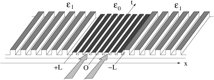
Figure 1: Example of a physical situation where the model (1) applies where $t$ is the propagation direction and $V$ is proportionnal to the dielectric constant difference $\epsilon_{0}-\epsilon_{1}$.

This problem has promising application to nonlinear optics where it applies to the propagation in the direction $t$, and tranverse modulation along $x$, of the envelope of a laser beam in a fiber Bragg grating (in Kerr regime) kivsh-agra when different types of fibers are used: self-focusing nonlinearity with dielectric constant $\epsilon_{1}$ outside $[-L,+L]$, self-defocusing with $\epsilon_{0}>\epsilon_{1}$ inside. The periodic medium extending in $|x|>L$ acts as a Bragg mirror for the tranverse modulation and the resulting Bragg grating resonator is sketched on figure 1. The arrows show the injected radiation.

The domain of spatial solitons in fiber Bragg gratings is rich of recent results, see e.g. kivshar ; khomeriki , with nice experimental evidence of soliton formation mandelik and recent experiments which demonstrated the existence of discrete stationnary gap solitons expe . On the theoretical side, an interesting proposal of khomeriki is to generate discrete gap solitons by boundary driving a Bragg grating above the cut-off. The aproach uses the theory of nonlinear supratransmission nst extended to the case when the forbidden band results from the discrete nature of the medium.

In the quasi-continous case (large number of fibers and weak coupling), the device of fig.1 will be shown to be a means to generate gap solitons by continuous wave (cw) input radiation at a flux intensity given explicitely in terms of the dimensions of the potential well depth $V$ (or the dielectric constant varaition $\epsilon_{0}-\epsilon_{1}$). As an illustration, fig.2 shows the evolution of the fundamental mode at the threshold for which the input envelope is indeed cw-like and experiences an instability generating the gap soliton.

Figure 2: Profile of $F=|\psi|^{2}$ for the fundamental 0-mode initial datum at threshold amplitude in the case $V=1$ and $L=4$.

The threshold vaues are explicitely calculated for the entire set of nonlinear states. Finally we demonstrate that the linear small amplitude limit maps continuously the nonlinear states to the linear ones.

We shall need to refer to the linear eigenstates that read in the odd case

$$|x|\leq L\ :\ \psi=A\,e^{-i\omega t}\sin(kx)\ ,$$

$$|x|\geq L\ :\ \psi=A\,e^{-i\omega t}\sin(kL)e^{-\kappa(|x|-L)}\ ,$$

$$k^{2}=V\sin(kL)\ , \tan(kL)<0\ .$$ (2)

and in the even case

$$|x|\leq L\ :\ \psi=A\,,e^{-i\omega t}\cos(kx)\ ,$$

$$|x|\geq L\ :\ \psi=A\,e^{-i\omega t}\cos(kL)e^{-\kappa(|x|-L)}\ ,$$

$$k^{2}=V\cos(kL)\ , \tan(kL)>0\ ,$$ (3)

for $\omega=k^{2}<V$ and $\kappa^{2}=V-\omega$, and for arbitrary amplitude $A$.

Nonlinear states.

As learned from carr , the main tool to derive the nonlinear states is to connect a periodic solution inside the well to a static one-soliton tail outside. We make use of the fundamental solutions of NLS in terms of Jacobi elliptic functions for both symmetric (even) and antisymmetric (odd) cases jacobi .

First, outside the potential well we have the common soliton tails given by (still with $\kappa^{2}=V-\omega$ and $\omega<V$)

$$|x|\geq L,\quad\psi=\frac{\kappa\sqrt{2}\,e^{-i\omega t}}{\cosh[\kappa(|x|-L+d)]}\ ,$$ (4)

which replaces the two evanescent waves of the linear case. Note that the function $(-\psi)$ is also solution, a property which must be used to conveniently connect the solution inside to the outside tails.

Inside the well we use the basic solution

$$|x|\leq L,\quad\psi=\mu A\,e^{-i\omega t}\,\rm sn(A^{\prime}x+x_{0},\mu).$$ (5)

Here and in the following the amplitude $A$ is real-valued and positive and we define the new constant $A^{\prime}$ by $A=A^{\prime}\sqrt{2}$. By convenient choices of the constant $x_{0}$ we shall obtain both the odd and even solutions in the well.

This function $\psi$ is a solution of (1) if (necessary condition)

$$\omega^{2}=\frac{1}{2}A^{2}(1+\mu^{2}),$$ (6)

which links the frequency $\omega$ to the modulus $\mu$ of the elliptic functions. The requirement $\omega<V$ for a bound state implies that the modulus $\mu$ cannot exceed a maximum value $\mu_{m}$

$$\mu\leq(2V/A^{2}-1)^{1/2}=\mu_{m}.$$ (7)

We discovered that it is necessary to work with expressions of the solution for moduli $\mu>1$, performed by means of the identity $\mu\,\rm sn(u,\mu)=\,\rm sn(\mu u,1/\mu)$. The solutions for $\mu<1$ can be easily written down but either they do not contribute to the spectrum or they have their exact conterpart with $\mu>1$.

Odd solutions.

In the range $\mu\in[1,\mu_{m}]$ we define the following solution inside the well

$$|x|\leq L,\quad\psi=A\,e^{-i\omega t}\,\rm sn(\mu A^{\prime}x,\frac{1}{\mu})\ .$$ (8)

In order to obtain sufficient conditions for the set (8) (4) to be a solution of (1), we need to ensure continuity of the solution and its derivative in $x=\pm L$. This provides the admissible discrete set of moduli $\mu$ which, after some algebra, must solve

$$\mu^{2} \,\rm cn^{2}(b,\frac{1}{\mu})\,\rm dn^{2}(b,\frac{1}{\mu})=$$

$$\,\rm sn^{2}(b,\frac{1}{\mu})\left[\frac{2V}{A^{2}}-(1+\mu^{2})-\,\rm sn^{2}(b,\frac{1}{\mu})\right],$$ (9)

where the function $b$ is defined as

$$b=\mu A^{\prime}L.$$ (10)

Then the shift $d$ of the tail position for each solution $\mu$ of the above equation, is given by

$$A|\,\rm sn(b,\frac{1}{\mu})|=\frac{\kappa\sqrt{2}}{\cosh(\kappa d)}.$$ (11)

As for the linear case we must add a consistency condition which ensures the continuity of the derivatives. It is just a matter of careful reading of all possible cases to obtain the condition

$$\,\rm sn(b,\frac{1}{\mu})\,\rm cn(b,\frac{1}{\mu})\,\rm dn(b,\frac{1}{\mu})<0,$$ (12)

for the solution $\mu$ of (Odd solutions.) to be acceptable.

Even solutions.

Still with $\mu\in[1,\mu_{m}]$ we define

$$|x|<L,\quad\psi=A\,e^{-i\omega t}\,\rm sn(\mu A^{\prime}x+K(\frac{1}{\mu}),\frac{1}{\mu})\ .$$ (13)

obtained from (5) by the translation $x_{0}=K(1/\mu)/\mu$ where $K$ is the complete elliptic integral of the first kind. In that case the continuity conditions give the admissible set of moduli as solutions of (Odd solutions.) with now

$$b=\mu A^{\prime}L+K(\frac{1}{\mu})$$ (14)

and the consequent definition (11) of $d$. The consistency condition (12) still holds here with the above function $b$.

Note that in both expressions (8) and (13), the parameter $A$ does represent the maximum value of the amplitude of the solution, reached at $x=0$ for the even states (13) and at $x=K(1/\mu)$ for the odd states (8).

Example.

The figure 3 shows the solutions of the equations (Odd solutions.) for $V=1$ and $L=4$ in the odd and even cases, for which the associated linear problem possess 3 eigenstates (dashed lines). The 3 curves show the dependency of the eigenvalue of each nonlinear extension of the linear levels in terms of the amplitude $A$. These eigenvalues are given by the expression (6) for each solution $\mu$ of (Odd solutions.), in both cases (10) and (14), equations that are solved numerically (like in the linear case).

Figure 3: Dependence of the eigenvalues $\omega$ in terms of the amplitude for $V=1$ and $L=4$. Crosses indicate the values of amplitude threshold and the dashed curve is the prediction of global threshold (19).

The next figure 4 displays the three states for $V=1$ in the linear and nonlinear case corresponding to particular choices of amplitudes and frequencies as indicated on the graphs. These are the plots of the solutions (8) and (13), compared to the linear eigenfunctions (2) and (3).

LINEAR NONLINEAR

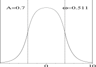
Figure 4: Examples of linear and nonlinear states, for $V=1$, with amplitudes and frequencies as indicated. The same vertical scale is used for linear and nonlinear figures.

There are two fundamental properties of this “nonlinear spectrum” that we demonstrate hereafter. It is first the evident natural property to reach the linear spectrum for vanishing amplitudes. This explains in particular why we have the same number of states as the linear levels. Second all three curves are seen to stop at some threshold amplitude which can be exactly computed, as shown by the dashed curve on figure 3 and the crosses which are the predicted thresholds.

Linear limit.

To demonstrate in general that the nonlinear spectrum goes to the linear one in the limit $A\to 0$, it is crucial to evaluate the limits keeping the product $A\mu$ finite. Actually defining

$$k=\frac{A}{\sqrt{2}}\mu,$$ (15)

we can easily obtain ($A=A^{\prime}\sqrt{2}$)

$$A\,\rm sn(\mu A^{\prime}x,1/\mu)\underset{A\to 0}{\sim}A\sin(kx),$$ (16)

which proves that the nonlinear odd states (8) tend to the linear ones in the limit $A\to 0$. The same property holds naturally for the nonlinear even states (13) by using $\,\rm sn(u+K(\nu),\nu)=\,\rm cd(u,\nu)$ and $\,\rm cd(u,0)=\cos(u)$ together with (16) above.

These results show in particular that the “nonlinear wave number” is the quantity $k=A^{\prime}\mu$ and thus that the relation (6) must be read $\omega^{2}=k^{2}+A^{2}/2$ that tends to the linear dispersion relation $\omega^{2}=k^{2}$ in the small amplitude limit.

Nonlinear tunneling.

More interesting is the existence of a threshold amplitude (or population threshold) beyond which gap solitons are emitted outside the well hence realizing a classical nonlinear tunneling. This is the result of an instability, as described in jl-pla , which takes place as soon as the amplitude $A$ is such that the soliton tails (4) reaches its maximum value in $|x|=L$, i.e. $d=0$.

In order to derive the analytic expression of the thresholds postions $\{A_{s},\omega_{s}\}$ for each branch $\omega(A)$, we express the continuity conditions in $|x|=L$ in the case $d=0$. The threshold is thus obtained as a particular solution of the equation for the state (Odd solutions.) for which both sides vanish altogether (successively for the odd and even states), namely

$$\,\rm cn^{2}(b,\frac{1}{\mu})\,\rm dn^{2}(b,\frac{1}{\mu})=0,$$ (17)

$$\frac{2V}{A^{2}}-(1+\mu^{2})-\,\rm sn^{2}(b,\frac{1}{\mu})=0.$$ (18)

where $b$ is given by (10) for the odd solutions and by (14) for the even ones.

It is then a matter of algebraic manipulations to demonstrate that the solutions $\{A_{s},\ \mu_{s}\}$ of the above equations globally satisfy

$$A_{s}^{2}=\frac{2V}{2+\mu_{s}^{2}}=2(V-\omega_{s}),$$ (19)

where $\mu_{s}$ is obtained by solving for the odd case

$$\,\rm sn^{2}(L\mu\sqrt{\frac{V}{\mu^{2}+2}},\frac{1}{\mu})=1,$$ (20)

and for the even case

$$\,\rm sn^{2}(L\mu\sqrt{\frac{V}{\mu^{2}+2}}+K(\frac{1}{\mu}),\frac{1}{\mu})=1.$$ (21)

Note that the solutions $\{A_{s},\ \mu_{s}\}$ of these equation must obey requirement (7) which is checked a posteriori.

The dashed curve of fig. 3 is the plot of (19) for $V=1$ and $L=4$, and the crosses are obtained by solving (20) and (21) numerically.

The above pocedure does not furnishes the threshold corresponding to the fundamental level. Indeed it misses the particular solution

$$\mu_{s}=1,\quad A_{s}^{2}=\frac{2}{3}V,$$ (22)

which is effectively a solution of (17)(18) from the property

$$\lim_{\mu\to 1}\left\{\,\rm sn(a+K(\frac{1}{\mu}),\frac{1}{\mu})\right\}=1,$$ (23)

for any real-valued $a$. In that case the “dispersion relation” (6) provides $\omega_{s}=A_{s}^{2}$. Note that the threshold amplitude $A_{s}$ does not depend on the width $2L$ of the well.

This solution is particularly interesting in view of applications to the fiber guide grating of fig.1. Indeed in that case the corresponding expression (13) is the constant amplitude field $\psi=A_{s}e^{-i\omega_{s}t}$ (which is trivialy a solution of (1)). Injecting then in the medium (as indicated by the arrows on fig.1) a cw-laser beam of (normalized) intensity flux $A_{s}^{2}$ constant along the tranverse $x$-direction for $x\in[-L,+L]$, one would generate a gap soliton propagating outside the well, as displayed in fig. 2. Such simulation can be reproduced ad libidum for input data constant in $[-L,+L]$ and exponentially vanishing outside. As soon as the amplitude exceeds the threshold $A_{s}$, one obtains tunelling by soliton emission.

It is clear that the present formalism has been developped for continuous envelopes $\psi(x,t)$, which requires a large number of fiber guides and weak transverse coupling. An interesting extension is then the discrete situation with the open question of the discrete states solutions.

Perspectives and conclusion.

We have so far demonstrated the existence of “nonlinear eigenstates”, exact solutions of the NLS model (1), that are remarkably stable (numerical simulations did not show any deviation from the exact expressions up to times when numerical errors become sensible, i.e. $10^{3}$ to $10^{4}$ for our scheme) as soon as their amplitudes do not exceed a threshold explicitely evaluated in terms of the well height for each mode. These states reproduce exactly, in the small amplitude limit, the usual eigenstates of the Shrödinger equation in a potential well.

Above the threshold amplitude, a “nonlinear tunneling” (macroscopic, classical) occurs by the emission of gap solitons outside the well. This generic property suggests a “gap soliton generator” by the device sketched in fig.1, more especially as the fundamental level, close to the threshold, behaves as a cw-field.

The approach applies straightforwardly to a model where the inside of the well would obey the linear Schrödinger equation. This in view of applications to a resonator device with Bragg medium playing the role of the mirrors, a subject under study now.

Another natural question is the properties of the nonlinear states when the inside of the well presents an attractive (focusing) nonlinearity (as the outside medium). In that case, similar states are defined in terms of Jacobi $\,\rm cn$-functions carr but we have observed that they experience modulational instability before reaching the threshold amplitude. In the other case when the whole medium is defocusing, the outside tails are of cosech-type and thus can match any amplitude of the nonlinear state, hence there is no threshold and no gap soliton generation. Thus the management of the nonlinearity chosen in (1) is a means for sabilizing the nonlinear states and ensuring a threshold for soliton generation.

We report to future studies the important question of the analytical proof of the stability of those states, including the mathematical derivation of the instability criterion above the threshold amplitude. Note finally that, in the threshold regions, the states are degenerated: two solutions coexist at the same frequency with slightly different amplitudes as seen on fig.3.

References

- (1) L.D. Carr, K.W. Mahmud, W.P. Reinhardt, Phys Rev A 64 (2001) 033603
- (2) Y.S. Kivshar, G.P. Agrawall, Optical Solitons: From Fibers to Photonic Crystals, Academic Press, San Diego, CA (2003)
- (3) A.A. Sukhorukov, Y.S. Kivshar, Phys Rev E 65 (2002) 036609
- (4) D. Mandelik, H.S. Eisenberg, Y. Silberberg, R. Morandotti, J.S. Aitchison, Phys Rev Lett 90 (2003) 053902
- (5) A.A. Sukhorukov, Y.S. Kivshar, Opt Lett 28 (2003) 2345
- (6) D. Mandelik, R. Morandotti, J.S. Aitchison, Y. Silberberg, Gap solitons in waveguide arrays to appear in Phys Rev Lett
- (7) R. Khomeriki, Phys Rev Lett 92 (2004) 063905
- (8) F. Geniet, J. Leon, Phys Rev Lett 89 (2002) 134102; and J Phys Cond Matt 15 (2003) 2933
- (9) L.D. Carr, C.W. Clark, W.P. Reinhardt, Phys Rev A 62 (2000) 063610 and 063611
- (10) J. Leon, Phys Lett A 319 (2003) 130