Reduced Singular Solutions of EPDiff Equations
on Manifolds with Symmetry

Abstract

The EPDiff equation governs geodesic flow on the diffeomorphisms with respect to a chosen metric, which is typically a Sobolev norm on the tangent space of vector fields. EPDiff admits a remarkable ansatz for its singular solutions, called “diffeons,” whose momenta are supported on embedded subspaces of the ambient space. Diffeons are true solitons for some choices of the norm. The diffeon solution ansatz is a momentum map. Consequently. the diffeons evolve according to canonical Hamiltonian equations. We examine diffeon solutions on Einstein spaces that are “mostly” symmetric, i.e., whose quotient by a subgroup of the isometry group is 1-dimensional. An example is the two-sphere, whose isometry group ${\mathrm{SO}}(3)$ contains $S^{1}$. In this situation, the singular diffeons (called “Puckons”) are supported on latitudes (“girdles”) of the sphere. For this $S^{1}$ symmetry of the two-sphere, the canonical Hamiltonian dynamics for Puckons reduces from integral partial differential equations to a dynamical system of ordinary differential equations for their colatitudes. Explicit examples are computed numerically for the motion and interaction of the Puckons on the sphere with respect to the $H^{1}$ norm. We analyse this case and several other 2-dimensional examples. From consideration of these 2-dimensional spaces, we outline the theory for reduction of diffeons on a general manifold possessing a metric equivalent to the warped product of the line with the bi-invariant metric of a Lie group.

1 Introduction

1.1 Motivation and Problem Statement

When the Schumacher-Levi comet broke into a string of fragments that collided with Jupiter in July 1994, each of the impacts created a circularly symmetric expanding “ripple” spreading out into the gaseous sphere of Jupiter. If the collision had occurred instead with an Earth-like planet which was entirely covered by a shallow layer of water, it would have produced a sequence of strongly nonlinear circular traveling-wave ripples spreading out from a point source on the spherical surface, propagating to the antipodal point, then reflecting back in the opposite direction and colliding head-on with the trailing waves.

Neglecting planetary rotation and assuming the energy was mainly kinetic in this situation would produce an approximate description of these strongly nonlinear shallow water waves as solitary waves governed by the Camassa-Holm (CH) equation [3], written on the sphere. The momenta for these solitary waves on the surface of the sphere would be concentrated on a series of coaxial circles which could each be regarded as a latitude encircling the axis running from the point of impact to the antipodal point. These concentrations of momentum on latitudes are singular solutions of the EPDiff equation, which is a geometrical extension of the CH equation for shallow water waves to higher dimensions.

Previously, the CH equation and its extension EPDiff have been solved analytically for the interactions of such waves on the real line in one dimension [3], as radially-symmetric rotating concentric circles on the two-dimensional plane [8] and numerically in two dimensions and three dimensions, for a variety of initial value problems [10]. In cases with one-dimensional linear, or radial symmetry, these dynamics reduce to ordinary differential equations (ODEs). Here we consider the corresponding reduction for singular wave motion on the surface of the sphere for EPDiff with respect to the $H^{1}$ norm and we discuss its generalisations for other surfaces of constant curvature.

In each case, we derive the symmetry which reduces the dynamics of the singular solutions of the EPDiff equation to a system of ODEs. We also provide explicit numerical results for the interactions of these singular EPDiff solutions in the case of Puckon motion as concentric latitudes moving on the sphere.

1.2 Review and Generalisation of the Camassa-Holm Equations to EPDiff

The dispersionless Camassa-Holm (CH) equations [3] for one-dimensional shallow water waves arise as stationary points of the kinetic energy functional given by the Sobolev (2,1)-norm

$$\ell : W^{2,1}(\mathbb{R})\longrightarrow\mathbb{R}\,,$$

$$\ell[u] = \int_{\mathbb{R}}\left(u(x)^{2}+u_{x}(x)^{2}\right)\mathrm{d}x\,,$$

subject to velocity variations in the Euler-Poincaré form [6]

$$\delta u=\dot{\zeta}+[\zeta,u]\,,$$

where $u,\zeta\in\mathfrak{g}$, and $\mathfrak{g}$ consists of the vector fields on the real line, with Lie bracket $[\cdot,\cdot]$ given by

$$[v,w]=vw_{x}-wv_{x}=\mathrm{ad}_{v}w\,.$$

The dispersionless CH equations themselves are thus given by the following system for velocity $u$ and its dual momentum $m$,

$$\dot{m} = -\mathrm{ad}_{u}^{*}m=-(m\partial_{x}+\partial_{x}m)u\,,$$

$$\hbox{where}\quad m = \frac{\delta\ell}{\delta u}=u-u_{xx}=u+\Delta u\,,$$

$$\Longrightarrow\quad u = G*m=\int_{\mathbb{R}}G(x-y)m(y)dy\,,$$

and $G(x)=\frac{1}{2}e^{-|x|}$ is the Green’s function for the Helmholtz operator $1-\partial_{x}^{2}$ on the real line. We remark that here we are using the convention that the Laplacian in 1D is given by

$$\Delta u=-u_{xx}.$$

The sign comes from regarding the Laplacian as $\partial_{x}^{*}\partial_{x}$, where $\partial_{x}^{*}$ is the $L^{2}$ adjoint of the derivative operator $\partial_{x}$.

To put the dispersionless CH equations onto a general Riemannian manifold $(M,\left\langle\cdot,\cdot\right\rangle)$ with dim$M=n$ and Levi-Civita connection $\nabla$, we work with the functional on the space of weakly differentiable square-integrable vector fields

$$\ell : W^{2,1}\mathcal{X}(M)\longrightarrow\mathbb{R}$$

$$\ell[u] = \int_{M}\left(|u|^{2}+|\nabla u|^{2}\right)\mathrm{d}vol.$$

Again, we consider the stationary points of $\ell$ with respect to variations of the Euler-Poincaré form

$$\delta{u}=\dot{\zeta}+[\zeta,u]\,.$$

This requirement yields the EPDiff equations, for “Euler-Poincaré equations on the diffeomorphisms,” given by the system,

$$\dot{m}=-\mathrm{ad}_{u}^{*}m\,,\quad\hbox{where}\quad m=\frac{\delta\ell}{\delta u}=u+\Delta^{\nabla}u\,.$$ (1)

Here we denote

$$\Delta^{\nabla}=\nabla^{*}\nabla$$

for the connection Laplacian with respect to the metric and we assume homogeneous boundary conditions.

Diffeons: Singular solutions for EPDiff.

The EPDiff equation (1) has Lie-Poisson Hamiltonian structure in the momentum variable $m$ and satisfies a remarkable ansatz for its singular solutions, which are called “diffeons,”

$$m(t,x)=\sum_{i=1}^{N}\int_{S_{i}}P_{i}(t,s_{i})\delta(x-R_{i}(t,s_{i}))\,ds_{i}\,.$$ (2)

The diffeon singular solutions of EPDiff are vector-valued functions supported in $M$ on a set of $N$ surfaces (or curves) of codimension $(n-k)$ for $s\in M^{k}\subset M$ with dim$M^{k}=k<n$. For example, diffeons may be supported on sets of points ($k=0$), curves ($k=1$), or surfaces ($k=2$) in three dimensions. These support sets of $m$ move with the fluid velocity $u=G*m$; so the coordinates $s\in M^{k}\subset M$ are Lagrangian fluid labels. The Green’s function $G$ for the operator $1+\Delta^{\nabla}$ is continuous, but it has a jump in its derivative on the support set that advects with the velocity $u=G*m$ under the evolution of EPDiff. In fluid dynamics, a jump in derivative which moves with the flow is called a “contact discontinuity” [12]. The relationship of the singular solutions of EPDiff equation (1) to fluid dynamics is illuminated by rewriting equation (1) in “Riemann-invariant form,”

$$\frac{d}{dt}(m\cdot{dx}\otimes{dvol})=0\,,\quad\hbox{along}\quad\frac{dx}{dt}=u=G*m\,.$$

The diffeon singular solution ansatz (2) was first discovered as the “peakon” solutions for CH motion on the real line in [3]. This was generalised to motion in higher dimensions in [9] and was shown to be a momentum map in [5]. As a result of the singular solution ansatz being a momentum map, the $2N$ variables $P_{i},R_{i},$ satisfy Hamilton’s canonical equations. In general, these are integro-partial differential equations for the canonically conjugate diffeon parameters $P_{i}(t,s_{i}),R_{i}(t,s_{i})$ in (2) with $i=1,\dots,N$.

1.3 Aim of the paper

This paper will be concerned with examining diffeon solutions of the EPDiff equations (1) on Einstein manifolds that are “mostly” symmetric, i.e., that have a group acting by isometries so that the orbits have co-dimension 1 in the manifold except on a set of measure zero, and hence the quotient of the manifold by the group is 1-dimensional.

Thus, we are interested in identifying and analysing cases where imposing an additional translation symmetry on the solution reduces the canonical Hamiltonian dynamics of the singular solutions of the EPDiff on Einstein manifolds from integro-partial differential equations to ordinary differential equations for $P_{i}(t),R_{i}(t)$. We shall then analyse some of the properties of those canonical equations and examine their numerical solutions.

We begin by noting some simplifications of the EPDiff equations when restricted to Einstein spaces. These simplifications take advantage of the relation between the connection Laplacian and the Hodge Laplacian, the latter of which is easier to compute. Knowing the EPDiff equations in 1-dimension, we move up to the Einstein spaces in two dimensions.

The first manifold we study is the 2-sphere, which has the familiar group action formed by rotations about a fixed axis. Thus we construct “Puckons,” which are singular solutions of the EPDiff equations supported on concentric circular latitudes of the 2-sphere. The name “Puckon” (as opposed to “peakon”) arises from the famous boast by Shakespeare’s character, Puck, in A Midsummer Night’s Dream, that he would, “put a girdle round about the earth in forty minutes.” The case of rotationally symmetric singular solutions of EPDiff in the Euclidean plane has already been discussed in [8], so we proceed to examine the hyperbolic plane, which has a rich isometry group. However, the diffeon dynamics on the unbounded hyperbolic plane affords little opportunity for multiple diffeon interactions and does not admit periodic behaviour. Richer opportunities for diffeon dynamics and interactions in hyperbolic spaces are offered in the context of Teichmüller theory, which is, however, beyond the scope of the present work.

From consideration of these 2-dimensional spaces, we sketch how one might develop the theory for the general manifold which possesses a metric equivalent to the warped product of the line with the bi-invariant metric of a Lie group.

1.4 Plan of the paper

After briefly recalling the essentials needed from the theory of Einstein manifolds in section 2, we begin in section 3 by reducing the singular solutions of EPDiff to a canonical Hamiltonian dynamical system for the simplest Einstein manifold – namely, motion on a sphere of singular EPDiff solutions supported on concentric circular latitudes, or “girdles.” These new singular solutions girdling the sphere are the “Puckons.” Although the canonical reduction is guaranteed by the momentum map property of EPDiff, the reduction of its singular diffeon solutions for Puckons is given in detail, so it may be used to confirm the numerical results for the interactions of Puckons on the sphere described in Section 2. Section 5 generalises the Puckons to other surfaces that are Einstein manifolds with a translation symmetry. Section 6 incorporates these ideas into the theory of warped products.

2 The EPDiff Equations on Einstein Spaces

The operator

$$\Delta^{\nabla}+\,{\mathrm{l}\!\!\!{1}}$$

arises in the following context in Riemannian geometry.

Definition 2.1

On any given Riemannian manifold, the musical isomorphisms are defined to be the Riesz representation and inverse maps with respect to the metric:

$$\sharp:\mathrm{T}^{*}M \longrightarrow \mathrm{T}M$$

$$\left\langle\alpha^{\sharp},w\right\rangle = \alpha(w)$$

$$\flat:\mathrm{T}M \longrightarrow \mathrm{T}^{*}M$$

$$v_{\flat}(w) = \left\langle v,w\right\rangle.$$

In Riemannian geometry, the Levi-Civita connection respects the musical isomorphisms, namely for $v,w\in\mathcal{X}(M)$ and $\alpha\in{\Omega^{1}}(M)$:

$$(\nabla_{v}w)_{\flat} = \nabla_{v}(w_{\flat})$$

$$(\nabla_{v}\alpha)^{\sharp} = \nabla_{v}(\alpha^{\sharp}).$$

Thus, the musical isomorphisms identify vector fields with 1-forms and allow them to be differentiated in the same way

The connection Laplacian on 1-forms satisfies the Bochner-Weitzenböck formula.

Theorem 2.2 (Bochner-Weitzenböck)

On a Riemannian manifold with Levi-Civita connection $\nabla$, any 1-form $\alpha$ satisfies

$$\Delta^{\mathrm{d}}\alpha=\Delta^{\nabla}\alpha+\mathrm{Ric}(\alpha)$$

where $\Delta^{\mathrm{d}}=\mathrm{d}^{*}\mathrm{d}+\mathrm{d}\mathrm{d}^{*}$ is the Hodge Laplacian formed from the exterior derivative $\mathrm{d}$ on forms and $\mathrm{Ric}$ is the Ricci curvature operator.

Now we restrict our attention to special forms of manifold, namely Einstein Manifolds.

Definition 2.3

An Einstein manifold is a Riemannian Manifold which satisfies

$$\mathrm{Ric}=k\,{\mathrm{l}\!\!\!{1}}$$

for some constant $k$.

On an Einstein manifold, one may scale the metric so that $k$ can be replaced by $-1,0,1$ depending on whether $k$ is negative, zero or positive respectively. Thus on an Einstein manifold, the Bochner-Weitzenböck formula becomes

$$\Delta^{\mathrm{d}}=\Delta^{\nabla}+\mathrm{sign}(k)\,{\mathrm{l}\!\!\!{1}}.$$

We restrict our study further to Einstein manifolds with positive $k$ (we shall call these positive Einstein manifolds) and scale to $k=1$. Thus we have

$$\Delta^{\mathrm{d}}=\Delta^{\nabla}+\,{\mathrm{l}\!\!\!{1}}.$$

The implication of this for the EPDiff Lagrangian on vector fields is as follows, for homogeneous boundary conditions:

$$\ell[{\mbox{\boldmath$u$}}] = \int_{M}\left(|{\mbox{\boldmath$u$}}|^{2}+|\nabla{\mbox{\boldmath$u$}}|^{2}\right)\mathrm{d}vol$$

$$= \int_{M}\left(|{\mbox{\boldmath$u$}}_{\flat}|^{2}+|\nabla{\mbox{\boldmath$u$}}_{\flat}|^{2}\right)\mathrm{d}vol$$

$$= \int_{M}\left\langle{\mbox{\boldmath$u$}}_{\flat},{\mbox{\boldmath$u$}}_{\flat}+\Delta^{\nabla}{\mbox{\boldmath$u$}}_{\flat}\right\rangle\mathrm{d}vol$$

$$= \int_{M}\left\langle{\mbox{\boldmath$u$}}_{\flat},\Delta^{\mathrm{d}}{\mbox{\boldmath$u$}}_{\flat}\right\rangle\mathrm{d}vol$$

$$\Big{(} = \int_{M}\left(|\mathrm{d}{\mbox{\boldmath$u$}}_{\flat}|^{2}+|\mathrm{d}^{*}{\mbox{\boldmath$u$}}_{\flat}|^{2}\right)\mathrm{d}vol\Big{)}.$$

Hence, finding the stationary points of Lagrangian $\ell$ with the usual Euler-Poincaré constraints on the variations implies the EPDiff equation system of equations (1) in the form

$$\dot{{\mbox{\boldmath$m$}}}=-\mathrm{ad}_{\mbox{\boldmath$u$}}^{*}{\mbox{\boldmath$m$}}\,,\quad\hbox{where}\quad{\mbox{\boldmath$m$}}=\Delta^{\mathrm{d}}{\mbox{\boldmath$u$}}_{\flat}\,.$$ (3)

These equations generalize the EPDiff equations to Einstein manifolds.

3 The EPDiff equations on the Sphere

In two dimensions, the only manifold with positive Einstein constant is the standard round sphere which we shall regard as the Riemann sphere. We use stereographic projections to identify the complex plane with the sphere whose North Pole is removed. This is equivalent to putting the metric

$$g=\frac{4}{(1+x^{2}+y^{2})^{2}}\left(\mathrm{d}x^{2}+\mathrm{d}y^{2}\right)=\frac{4}{(1+|z|^{2})^{2}}\mathrm{d}z\mathrm{d}\bar{z}$$

on the plane.

3.1 Rotationally Invariant Solutions

We shall examine vector-field solutions $u$ of EPDiff in (3) with

$$\int_{{\mathrm{S}^{2}}}\left\langle\Delta^{\mathrm{d}}{\mbox{\boldmath$u$}}_{\flat},\beta\right\rangle=\int_{C}\beta$$

for any smooth 1-form $\beta$ where $C$ is a circle of latitude on the sphere. The quantity ${\mbox{\boldmath$m$}}=\Delta^{\mathrm{d}}{\mbox{\boldmath$u$}}_{\flat}$ is a distribution, defined by its integration against a smooth function. Thus, we seek weak, or singular, solutions of EPDiff on the sphere. We change coordinates on the sphere to assist us in this search. The metric on $\mathbb{R}^{2}\backslash{0}$ in polar coordinates is $\mathrm{d}r^{2}+r^{2}\mathrm{d}\theta$. Thus we can regard the sphere minus both poles as $\mathbb{R}^{2}\backslash 0$ with the metric

$$g_{\,\mathbb{S}}=\rho^{2}\left(\mathrm{d}r^{2}+r^{2}\mathrm{d}\theta^{2}\right)\,,\quad\hbox{where}\quad\rho=\frac{2}{(1+r^{2})}\,.$$

Green’s function for the Helmholtz operator on the Riemann sphere.

We now seek solutions to the equation

$$\Delta^{\mathrm{d}}{\mbox{\boldmath$u$}}_{\flat}=\delta(r-R)(k_{1}\mathrm{d}r+k_{2}\mathrm{d}\theta)$$ (4)

where $R,k_{1},k_{2}$ are constants. Let us assume that the velocity one-form ${\mbox{\boldmath$u$}}_{\flat}$ is invariant under rotations of the sphere about the axis joining North and South Poles and is radial, i.e. we must solve

$${\mbox{\boldmath$u$}}_{\flat} = a(r)\mathrm{d}r,$$ (5)

$$\Delta^{\mathrm{d}}{\mbox{\boldmath$u$}}_{\flat} = P\frac{\delta(r-R)}{r\rho(R)^{2}}\mathrm{d}r.$$ (6)

Let us first solve the Green’s function equation

$$\Delta^{\mathrm{d}}(G(r,R)\mathrm{d}r)=\frac{\delta(r-R)}{r}\mathrm{d}r\,,$$

for one recognises that the single diffeon velocity is proportional to the Green’s function, i.e.,

$$a(r)=PG(r,R)\,.$$

To solve explicitly for the Green’s function in our present case, we begin by recalling

$$\Delta^{\mathrm{d}}G(r,R)\mathrm{d}r=-\,\frac{\partial}{\partial{r}}\left(\frac{(1+r^{2})^{2}}{4r}\frac{\partial{(rG(r,R))}}{\partial{r}}\right)\mathrm{d}r\,.$$

Integrating the Green’s function equation using this expression yields

$$G(r,R)\mathrm{d}r=\left(\frac{A_{1}}{r}+\frac{2A_{2}}{r(1+r^{2})}+\frac{2}{r(1+\max(r,R)^{2})}\right)\mathrm{d}r\,,$$

for constants $A_{1},A_{2}$. In particular, we can remove the singularities at $r=0$ and $r=\infty$ by setting $A_{1}=0$ and

$$A_{2}=-\,\frac{1}{R(1+R^{2})}\,,$$

whence

$$G(r,R)\mathrm{d}r=\frac{2\min(r,R)^{2}}{rR(1+r^{2})(1+R^{2})}\mathrm{d}r.$$

Similarly, the solution to

$$\Delta^{\mathrm{d}}\tilde{G}(r,R)\mathrm{d}\theta=R\delta(r-R)\mathrm{d}\theta$$

for the angular diffeon velocity component is

$$\tilde{G}(r,R)\mathrm{d}\theta=\frac{2R\min(r,R)^{2}}{r(1+r^{2})(1+R^{2})}\mathrm{d}\theta=R^{2}G(r,R)\mathrm{d}\theta\,.$$

Both $G$ and $\tilde{G}$ are continuous over the sphere, but each has a jump in derivative at $r=R$.

Thus, we have proved the following.

Proposition 3.1 (Radial Green’s function on the sphere)

The solution to (5,6) for the radial Green’s function on the sphere is

$$PG(r,R)\mathrm{d}r=\frac{2P\min(r,R)^{2}}{rR(1+r^{2})(1+R^{2})}\mathrm{d}r\,.$$

Solution ansatz for EPDiff on the sphere.

Following [9], we propose a solution ansatz for EPDiff velocity on the sphere as the following superposition of Green’s functions,

$$\eta=\sum_{i=1}^{N}P_{i}G_{R_{i}}\mathrm{d}r$$ (7)

where we denote

$$G_{R}(r)=RG(r,R).$$

and $P_{i}$, $R_{i}$ are $2N$ functions of time. The corresponding vector field dual to $\eta$ is

$${\mbox{\boldmath$u$}}=\sum_{i=1}^{N}\frac{1}{\rho^{2}}P_{i}G_{R_{i}}\partial_{r}$$ (8)

We pair the arbitrary smooth vector field $w=f\partial_{r}+g\partial_{\theta}$ on ${\mathrm{S}^{2}}$ with the EPDiff equation using the solution ansatz given by the one-form $\eta$ in equation (7). A direct calculation yields the following equations for the diffeon parameters,

Proposition 3.2 (Diffeon parameter equations on the sphere)

The equations for diffeon parameter evolution on the sphere are:

$$\dot{R_{i}} = \sum_{j=1}^{N}\left(\frac{P_{j}}{\rho(R_{i})^{2}\rho(R_{j})^{2}R_{j}}G(R_{i},R_{j})\right)$$ (9)

$$\dot{P}_{i} = -\sum_{j=1}^{N}\frac{P_{i}P_{j}}{\rho(R_{i})^{2}\rho(R_{j})^{2}}\left(\frac{\partial}{\partial{r}}G(r,R_{j})\bigg{|}_{r=R_{i}}+2R_{i}\rho(R_{i})G(R_{i},R_{j})\right).$$ (10)

Proof (by direct calculation):

$$0 = \frac{\partial}{\partial{t}}\left(\int_{{\mathrm{S}^{2}}}\Delta^{\mathrm{d}}\eta(w)\mathrm{d}vol\right)+\int_{{\mathrm{S}^{2}}}\Delta^{\mathrm{d}}\eta([w,{\mbox{\boldmath$u$}}])\mathrm{d}vol$$

$$= \frac{\partial}{\partial{t}}\left(\sum_{i=1}^{N}\int_{0}^{2\pi}\int_{0}^{\infty}\delta(r-R_{i})f(r,\theta)P_{i}\rho^{2}r\mathrm{d}r\mathrm{d}\theta\right)$$

$$+ \int_{0}^{2\pi}\sum_{i=1}^{N}\int_{0}^{\infty}\delta(r-R_{i})P_{i}\mathrm{d}r\left(\left[f(r,\theta)\partial_{r}+g(r,\theta)\partial_{\theta},\sum_{j=1}^{N}{\rho^{-2}}P_{j}G_{R_{j}}(r)\partial_{r}\right]\right)\rho^{2}r\mathrm{d}r\mathrm{d}\theta$$

$$= \frac{\partial}{\partial{t}}\left(\sum_{i=1}^{N}P_{i}\int_{0}^{2\pi}f(R_{i},\theta)\mathrm{d}\theta\right)$$

$$+ \sum_{i,j=1}^{N}R_{i}\int_{0}^{2\pi}\left(P_{j}G_{R_{j}}^{\prime}(R_{i})f(R_{i},\theta)+2P_{j}R_{i}\rho(R_{i})G_{R_{j}}(R_{i})f(R_{i},\theta)-P_{j}G_{R_{j}}(R_{i})f_{r}(R_{i},\theta)\right)P_{i}\mathrm{d}\theta$$

$$= \sum_{i=1}^{N}\int_{0}^{2\pi}(f_{r}(R_{i},\theta)\dot{R_{i}}P_{i}+\dot{P}_{i}f(R_{i},\theta))\mathrm{d}\theta$$

$$+ \sum_{i,j=1}^{N}R_{i}\int_{0}^{2\pi}\left(P_{j}G_{R_{j}}^{\prime}(R_{i})f(R_{i},\theta)+2P_{j}R_{i}\rho(R_{i})G_{R_{j}}(R_{i})f(R_{i},\theta)-P_{j}G_{R_{j}}(R_{i})f_{r}(R_{i},\theta)\right)P_{i}\mathrm{d}\theta$$

Comparing coefficients of $f$ and $f_{r}$ implies

$$0 = \dot{R_{i}}P_{i}-\sum_{j=1}^{N}\left(\frac{P_{i}P_{j}}{\rho(R_{i})^{2}\rho(R_{j})^{2}}G(R_{i},R_{j})\right)$$

$$0 = \dot{P}_{i}+\sum_{j=1}^{N}\frac{P_{i}P_{j}}{\rho(R_{i})^{2}\rho(R_{j})^{2}R_{j}}\left(G_{R_{j}}^{\prime}(R_{i})+2R_{i}\rho(R_{i})G_{R_{j}}(R_{i})\right)$$

This finishes the calculation of the diffeon parameter evolution equations (9,10). $\surd$

Proposition 3.3 (Canonical Hamiltonian form of diffeon parameter equations)

Evolution equations (9,10) for the diffeon parameters are equivalent to Hamilton’s canonical equations,

$$\dot{R_{i}}=\frac{1}{\pi}\frac{\partial{H}}{\partial{R_{i}}}\,,\quad\dot{P}_{i}=-\frac{1}{\pi}\frac{\partial{H}}{\partial{P_{i}}}\,,$$ (11)

with Hamiltonian function of $\mathbf{P}=(P_{1},\ldots,P_{N})$ and $\mathbf{R}=(R_{1},\ldots,P_{N})$ given by,

$$H(\mathbf{P},\mathbf{R})=\frac{\pi}{2}\sum_{i,j=1}^{N}\frac{P_{i}P_{j}G(R_{j},R_{i})}{\rho(R_{i})^{2}\rho(R_{j})^{2}}\,.$$ (12)

As explained in [5], this reduction of EPDiff to canonical Hamiltonian form for the diffeons is guaranteed, since the singular solution ansatz (2) is a momentum map. However, we shall require the explicit results for the numerical solutions in section 4.

Proof: We Legendre transform the Lagrangian $\ell$ into the Hamiltonian $H$ by setting

$$H({\mbox{\boldmath$m$}})=\int_{{\mathrm{S}^{2}}}{\mbox{\boldmath$m$}}({\mbox{\boldmath$u$}})\mathrm{d}vol-\ell[{\mbox{\boldmath$u$}}]$$

whence we find that

$$H({\mbox{\boldmath$m$}})=\frac{1}{2}\int_{{\mathrm{S}^{2}}}{\mbox{\boldmath$m$}}({\mbox{\boldmath$u$}})\mathrm{d}vol$$

with

$${\mbox{\boldmath$m$}}=\Delta^{\mathrm{d}}{\mbox{\boldmath$u$}}_{\flat}.$$

We then express the velocity as the superposition of Green’s functions,

$${\mbox{\boldmath$u$}}_{\flat}=\eta=\sum_{i=1}^{N}\frac{1}{\rho(R_{i})^{2}}\frac{2P_{i}\min(r,R_{i})^{2}}{rR_{i}(1+r^{2})(1+R_{i}^{2})}\mathrm{d}r\,.$$

We set $k_{i}=P_{i}/(\rho(R_{i})^{2}R_{i})$, for $i=1,\dots,N$, and we evaluate the Hamiltonian on this solution with ${\mbox{\boldmath$m$}}=\Delta^{\mathrm{d}}\eta$ as

$$H({\mbox{\boldmath$m$}}) = \frac{1}{2}\int_{{\mathrm{S}^{2}}}\left\langle\eta,{\mbox{\boldmath$m$}}\right\rangle\mathrm{d}vol$$

$$= \frac{1}{2}\int_{0}^{2\pi}\int_{0}^{\infty}\sum_{i,j=1}^{N}\left\langle\frac{2k_{i}\min(r,R_{i})^{2}}{r(1+r^{2})(1+R_{i}^{2})}\mathrm{d}r,\Delta^{\mathrm{d}}\frac{2k_{j}\min(r,R_{j})^{2}}{r(1+r^{2})(1+R_{j}^{2})}\mathrm{d}r\right\rangle\rho^{2}r\mathrm{d}r\wedge\mathrm{d}\theta$$

$$= \frac{1}{2}\int_{0}^{2\pi}\int_{0}^{\infty}\sum_{i,j=1}^{N}\left\langle k_{i}G_{R_{i}}(r)\mathrm{d}r,k_{j}\delta(r-R_{j})\mathrm{d}r\right\rangle\rho^{2}r\mathrm{d}r\wedge\mathrm{d}\theta$$

$$= \frac{1}{2}\int_{0}^{2\pi}\sum_{i,j=1}^{N}k_{i}G_{R_{i}}(R_{j})k_{j}R_{j}\mathrm{d}\theta$$

$$= \frac{\pi}{2}\sum_{i,j=1}^{N}\frac{P_{i}P_{j}G(R_{i},R_{j})}{\rho(R_{i})^{2}\rho(R_{j})^{2}}.$$

The canonical equations for this Hamiltonian now recover the diffeon parameter evolution equations (9,10). $\surd$

Remark 3.4 (Remark on constant factors)

For convenience and brevity of writing, in what follows we shall often absorb into the time units any constant factors – such as $\pi$ in equations (11-12) – arising from integration over symmetry directions.

Definition 3.5 ($N$-Puckon)

The singular solution of EPDiff

$$\frac{\partial}{\partial{t}}\Delta^{\mathrm{d}}\eta = -\mathrm{ad}^{*}_{\eta^{\sharp}}\Delta^{\mathrm{d}}\eta\,,$$ (13)

is given on the Riemann sphere by a vector field $\eta$ satisfying

$$\Delta^{\mathrm{d}}\eta = \sum_{i=1}^{N}\frac{P_{i}}{\rho(R_{i})^{2}R_{i}}\delta(r-R_{i})\mathrm{d}r\,.$$ (14)

The support set of this (weak) solution of EPDiff on the Riemann sphere is a set of circular latitudes (girdles) at radii $R_{i}(t)$ with conjugate radial momenta $P_{i}(t)$, where $i=1,\dots,N$. Equation (14) constitutes a solution ansatz for the velocity vector field $\eta$, which will be called an $N$-Puckon solution.

3.2 The Basic Irrotational Puckon

Purpose.

This subsection derives explicit solutions for the parameters $P$ and $R$ of the single Puckon without rotation and examines its behaviour upon collapsing to the poles of the sphere.

The single irrotational Puckon.

Let us consider the case where $N=1$ and examine the motion of the basic Puckon without rotation. For $N=1$, the Hamiltonian (12) is given by

$$H(P,R)=\frac{1}{2}\frac{P^{2}G(R,R)}{\rho(R)^{4}}=\frac{P^{2}}{8}(1+R^{2})^{2}\,,$$

which follows because the Green’s function in this case is

$$G(R,R)=2\frac{\min(R,R)^{2}}{R^{2}(1+R^{2})^{2}}=\frac{2}{(1+R^{2})^{2}}\,.$$

Thus, upon restricting ourselves to the constant level set of the Hamiltonian defined by

$$H(P,R)=\frac{K^{2}}{2}$$

for constant $K$, we may solve for the momentum variable,

$$P=K\rho(R)=\frac{2K}{(1+R^{2})}\,.$$

Next, we note that the canonical coordinate equation

$$\dot{R}=\frac{\partial{H}}{\partial{P}}=\frac{P}{4}(1+R^{2})^{2}=\frac{K}{2}(1+R^{2})\,,$$

integrates to

$$R=\tan\left(\frac{K}{2}t+\frac{\varepsilon}{2}\right)\,.$$ (15)

Consequently, the single Puckon momentum is found as

$$P=K+K\cos\left({K}t+{\varepsilon}\right).$$ (16)

So far we have been using the stereographic projection to provide charts for the sphere. However we may easily pass from the coordinates $(r,\theta)$ obtained from stereographic projection to latitudinal-longitudinal coordinates $(\phi,\theta)$ where $r$ and $\phi$ are related by

$$r=\tan\left(\frac{\phi}{2}\right).$$

By this token, the colatitude $\phi=\Phi(t)$ of the peak of the Puckon evolves linearly in time as

$$\Phi(t)=Kt+\varepsilon.$$

Proposition 3.6 (Irrotational Puckon Solution)

The velocity vector field $v=\eta^{\sharp}$ generated by the irrotational Puckon motion is given in stereographic coordinates by

$${\mbox{\boldmath$u$}}=\frac{P}{4}\frac{\min(r,R)}{\max(r,R)}(1+r^{2})\partial_{r}\,.$$

This appears in latitudinal-longitudinal coordinates on the Riemann sphere, as follows,

$${\mbox{\boldmath$u$}}=\frac{K(1+\cos(Kt+\varepsilon))}{2}\frac{\min\left(\left|\tan\left(\frac{\phi}{2}\right)\right|,\left|\tan\left(\frac{K}{2}t+\frac{\varepsilon}{2}\right)\right|\right)}{\max\left(\left|\tan\left(\frac{\phi}{2}\right)\right|,\left|\tan\left(\frac{K}{2}t+\frac{\varepsilon}{2}\right)\right|\right)}\frac{\partial}{\partial{\phi}}.$$

Proof:

This result is obtained by direct substitution of solutions (15) and (16) for the diffeon parameters into the solution ansatz (8).

Remark 3.7 (Puckon peak)

The peak of the Puckon occurs when

$$\phi=\Phi(t)=Kt+\varepsilon,$$

(modulo behaviour at the poles), whence

$$|{\mbox{\boldmath$u$}}|_{{\mathrm{S}^{2}}}=\frac{|K|(1+\cos(Kt+\varepsilon))}{2}\,.$$

We still need to examine precisely what happens to the dynamics of a Puckon as it collides with itself at the poles.

Proposition 3.8 (Puckon behavior at the poles)

The Puckon bounces elastically, when it collides with itself at the poles.

Proof: We notice that $\dot{R}=K/2\neq 0$ at $R=0$ and by setting $U=1/R$ we see that at $U=0$, $\dot{U}=K/2\neq 0$. Similarly, one can show that $\dot{P}=0$ at both poles. Thus, the Puckon velocity is finite at the poles. Since Hamiltonian motion is time-reversible, the Puckon must bounce elastically, when it collides with itself at the poles.

3.3 Rotating Puckons

So far we have concentrated on singular EPDiff solutions on the sphere moving with only a radial component. Now we turn to examine the rotating $N$-Puckon, i.e. the solution of the following system of equations for $\eta$, cf. equations (4),

$$\Delta^{\mathrm{d}}\eta = \sum_{i=1}^{N}\frac{\delta(r-R_{i})}{\rho(R_{i})^{2}R_{i}}\left(P_{i}\mathrm{d}r+M_{i}\mathrm{d}\theta\right)\,,$$ (17)

$$\frac{\partial}{\partial{t}}\Delta^{\mathrm{d}}\eta = -\mathrm{ad}^{*}_{\eta^{\sharp}}\Delta^{\mathrm{d}}\eta\,,$$ (18)

in which $M_{i}(t)$ with $i=1,\dots,N$, are the angular momenta of the $N$ Puckons.

Proposition 3.9 (Canonical Hamiltonian equations for the rotating $N$-Puckon)

The equations for the rotating $N$-Puckon may be expressed as:

$$\dot{R}_{i} = \sum_{j=1}^{N}P_{j}F_{j}(R_{i})R_{j}R_{i}=\frac{\partial H}{\partial P_{i}}\,,$$ (19)

$$\dot{P}_{i} = -\sum_{j=1}^{N}\left(P_{i}P_{j}F_{j}^{\prime}(R_{i})R_{j}R_{i}+P_{i}P_{j}F_{j}(R_{i})R_{j}+M_{i}M_{j}F_{j}^{\prime}(R_{i})\right)=-\,\frac{\partial H}{\partial R_{i}}\,,$$ (20)

$$\dot{M}_{i} = 0\,,$$ (21)

where $F_{i}(R_{j})=F_{j}(R_{i})$ is defined in terms of the Green’s function $G$ as

$$F_{i}(R_{j})=\frac{G(R_{i},R_{j})}{\rho(R_{i})^{2}R_{i}\rho^{2}(R_{j})R_{j}}\,.$$

The last equation (21) expresses the conservation of the angular momentum of each Puckon. With $M_{i}$ constant, the first two equations (19) and (20) comprise Hamilton’s canonical equations with symmetry-reduced Hamiltonian

$$H(\mathbf{P},\mathbf{R};\mathbf{M}) = \frac{1}{2}\sum_{i,j=1}^{N}\left(P_{i}P_{j}R_{i}R_{j}+M_{i}M_{j}\right)F_{i}(R_{j})\,.$$ (22)

Proof.

First, we note that the velocity one-form corresponding to the momentum singular solution ansatz (17) is given by,

$$\eta = \sum_{i=1}^{N}\frac{G(r,R_{i})}{\rho(R_{i})^{2}}\left(P_{i}\mathrm{d}r+M_{i}r\mathrm{d}\theta\right)$$

Thus the velocity vector field $u$ dual to $\eta$ is given by

$$u = \sum_{i=1}^{N}\frac{G(r,R_{i})}{\rho(R_{i})^{2}R_{i}\rho^{2}r}\left(R_{i}P_{i}r\partial_{r}+M_{i}\partial_{\theta}\right).$$

To make our calculations more transparent, we collect terms and define notation as

$$F_{i}(r)=\frac{G(r,R_{i})}{\rho(R_{i})^{2}R_{i}\rho^{2}r},$$

so that

$${\mbox{\boldmath$u$}}=\sum_{i=1}^{N}F_{i}(r)\left(R_{i}P_{i}r\partial_{r}+M_{i}\partial_{\theta}\right)$$

and

$$\eta=\sum_{i=1}^{N}F_{i}(r)\rho^{2}r\left(R_{i}P_{i}\mathrm{d}r+M_{i}r\mathrm{d}\theta\right).$$

Note that the expression for $F_{i}$ is symmetric in $r$ and $R_{i}$, which implies the permutation symmetry,

$$F_{i}(R_{j})=F_{j}(R_{i}).$$

Now let $w=f\partial_{r}+g\partial_{\theta}$ be any smooth vector field on ${\mathrm{S}^{2}}$. Then, one computes the pairing

$$\int_{{\mathrm{S}^{2}}}\Delta^{\mathrm{d}}\eta(w)\mathrm{d}vol = \sum_{i=1}^{N}\int_{0}^{2\pi}\left(P_{i}f(R_{i},\theta)+M_{i}g(R_{i},\theta)\right)\mathrm{d}\theta.$$

Hence, the left hand side of the EPDiff equation becomes

$$\frac{\partial}{\partial{t}}\left(\int_{{\mathrm{S}^{2}}}\Delta^{\mathrm{d}}\eta(w)\mathrm{d}vol\right)=\sum_{i=1}^{N}\int_{0}^{2\pi}\left(\dot{P}_{i}f(R_{i},\theta)+P_{i}\dot{R}_{i}f_{r}(R_{i},\theta)+\dot{M}_{i}g(R_{i},\theta)+M_{i}\dot{R}_{i}g_{r}(R_{i},\theta)\right)\mathrm{d}\theta.$$

Now we need to calculate its right hand side.

$$\int_{{\mathrm{S}^{2}}}\Delta^{\mathrm{d}}\eta([w,{\mbox{\boldmath$u$}}])\mathrm{d}vol.$$

For this, we write the commutator,

$$[w,{\mbox{\boldmath$u$}}] = \sum_{i=1}^{N}\left(F_{i}^{\prime}R_{i}P_{i}rf+F_{i}R_{i}P_{i}f-F_{i}R_{i}P_{i}rf_{r}-F_{i}M_{i}f_{\theta}\right)\partial_{r}$$

$$+ \sum_{i=1}^{N}\left(fF_{i}^{\prime}M_{i}-F_{i}R_{i}P_{i}rg_{r}-F_{i}M_{i}g_{\theta}\right)\partial_{\theta}.$$

Now, by Stokes’ theorem, when we integrate over the whole sphere, the contribution due to $f_{\theta},g_{\theta}$ will be zero because $f,g$, the only components of the integration to depend on $\theta$, satisfy $f(r,0)=f(r,2\pi)$ etc. Thus

$$\int_{{\mathrm{S}^{2}}}\Delta^{\mathrm{d}}\eta([w,{\mbox{\boldmath$u$}}])\mathrm{d}vol$$

$$= \sum_{i,j=1}^{N}\int_{0}^{2\pi}\left(P_{i}F_{j}^{\prime}(R_{i})R_{j}P_{j}R_{i}f(R_{i},\theta)+P_{i}F_{j}(R_{i})R_{j}P_{j}f(R_{i},\theta)-P_{i}F_{j}(R_{i})R_{j}P_{j}R_{i}f_{r}(R_{i},\theta)\right)\mathrm{d}\theta$$

$$+\sum_{i,j=1}^{N}\int_{0}^{2\pi}\left(M_{i}F_{j}^{\prime}(R_{i})M_{j}f(R_{i},\theta)-M_{i}F_{j}(R_{i})R_{j}P_{j}R_{i}g_{r}(R_{i},\theta)\right)\mathrm{d}\theta.$$

Now to find the evolution equations for $P_{i},R_{i},M_{i}$ we need only compare the coefficients of $f,f_{r},g,g_{r}$ occurring in

$$0=\frac{\partial}{\partial{t}}\left(\int_{{\mathrm{S}^{2}}}\Delta^{\mathrm{d}}\eta(w)\mathrm{d}vol\right)+\int_{{\mathrm{S}^{2}}}\Delta^{\mathrm{d}}\eta([w,{\mbox{\boldmath$u$}}])\mathrm{d}vol\,.$$

From this comparison, one finds

$$0 = \dot{P}_{i}+\sum_{j=1}^{N}\Big{(}P_{i}F_{j}^{\prime}(R_{i})R_{j}P_{j}R_{i}+P_{i}F_{j}(R_{i})R_{j}P_{j}+M_{i}F_{j}^{\prime}(R_{i})M_{j}\Big{)}\,,$$

$$0 = P_{i}\dot{R}_{i}-\sum_{j=1}^{n}\Big{(}P_{i}F_{j}(R_{i})R_{j}P_{j}R_{i}\Big{)}\,,$$

$$0 = \dot{M}_{i}\,,$$

$$0 = M_{i}\dot{R}_{i}-\sum_{j=1}^{N}\Big{(}M_{i}F_{j}(R_{i})R_{j}P_{j}R_{i}\Big{)}\,,$$

in which the second and fourth equations provide the same information. We therefore obtain the evolution equations (19-21) for $P_{i},R_{i},M_{i}$ given in the statement of Proposition 3.9. $\surd$

Remark 3.10 (Verifying the Hamiltonian)

A simple check shows that if the Hamiltonian

$$H({\mbox{\boldmath$m$}})=\int_{{\mathrm{S}^{2}}}{\mbox{\boldmath$m$}}({\mbox{\boldmath$u$}})\mathrm{d}vol-\ell[{\mbox{\boldmath$u$}}]$$

is the Legendre transform of the Lagrangian $\ell$ then

$$H({\mbox{\boldmath$m$}}) = \frac{1}{2}\int_{{\mathrm{S}^{2}}}\left\langle\Delta^{\mathrm{d}}\eta,\eta\right\rangle\mathrm{d}vol$$

$$= 2\pi H(\mathbf{P},\mathbf{R};\mathbf{M})\,,$$

which is the Hamiltonian for the rotating $N$-Puckon in formula (22) of Proposition 3.9. As explained in [5], the reduction to canonical Hamiltonian form is guaranteed, since the singular solution ansatz (2) is a momentum map.

3.4 The Basic Rotating Puckon

Proposition 3.11 (Extremal radii of the basic rotating Puckon)

The motion of the basic rotating Puckon lies between the maximum and minimum values of $R$ on the Riemann plane given by,

$$R_{max/min} = \frac{2K\pm\sqrt{4K^{2}-M^{2}}}{M}\,,$$ (23)

assuming that $2K\geq{M}>0$.

Proof:

We $N=1$ in Hamiltonian (22) to find

$$H(P,R)=\frac{1}{16R^{2}}(1+R^{2})^{2}(P^{2}R^{2}+M^{2}).$$

We notice that for a rotating Puckon with $H=K^{2}=const$, the girdle of the Puckon cannot have zero radius unless $M=0$, in which case we return to the irrotational Puckon. Likewise, the girdle radius cannot be infinite unless again $M=0$. Thus, a rotating Puckon with $M\neq 0$ is constrained to lie between a maximum and a minimum radius. To find these extremal radii, we must solve

$$\frac{\partial{H}}{\partial{P}}=\frac{P}{8}(1+R^{2})^{2} = 0\,,$$

$$H=\frac{1}{16R^{2}}(1+R^{2})^{2}(P^{2}R^{2}+M^{2}) = K^{2}.$$

The first equation can only be solved by $P=0$; for which the second becomes

$$\frac{M^{2}}{16R^{2}}(1+R^{2})^{2}=K^{2}.$$

Assuming that $K$ and $M$ are both positive, we find that the maximum and minimum values of $R$ are the roots,

$$R_{max/min} = \frac{2K\pm\sqrt{4K^{2}-M^{2}}}{M}$$

This proves the proposition. $\surd$

Remark 3.12 (A single critical point)

We observe that if $M=2K$, then the Puckon is radially static at the equator and $P$ is identically zero. The solution $(P,R)=(0,1)$ is the only critical point of the Hamiltonian $H$ unless $M=0$ in which case the set defined by $P=0$ is the critical manifold.

Proposition 3.13 (Periodic motion of the basic rotating Puckon)

The motion of the rotating Puckon is periodic, with period $2\pi/\sqrt{2H}$ determined by the constant value of the Hamiltonian, $H$.

Proof using the colatitude representation of periodic rotating Puckon motion:

To investigate the motion of the rotating Puckon, we pass from stereographic coordinates to longitude-colatitude coordinates in which we put

$$R=\tan\frac{\Phi}{2}.$$

As we will see later in the general case, this does not alter the situation a great deal. For example, the momentum is given later in equation (32), after substituting $\sin$ for $\psi$. The Hamiltonian for the rotating Puckon on the sphere in longitude-colatitude coordinates is

$$H(P,\Phi)=\frac{1}{2}\left(P^{2}+\frac{M^{2}}{\sin^{2}\Phi}\right),$$ (24)

in which $\Phi$ and $P$ are canonically conjugate variables. Along the motion of the Puckon, $H$ is constant, say $H=K^{2}$. Thus, taking the positive branch for $P$

$$P=\sqrt{2K^{2}-\frac{M^{2}}{\sin^{2}\Phi}}$$

yields the equation for the colatitude

$$\dot{\Phi}=P=\sqrt{2K^{2}-\frac{M^{2}}{\sin^{2}\Phi}}.$$

Integration of this ODE implies that

$$t = \int_{\Phi(0)}^{\Phi(t)}\frac{\sin\Phi\,\mathrm{d}\Phi}{\sqrt{2K^{2}\sin^{2}\Phi-M^{2}}}$$

$$= \frac{1}{K\sqrt{2}}\left(\arccos\left(\frac{K\sqrt{2}\cos\Phi(t)}{\sqrt{2K^{2}-M^{2}}}\right)-\arccos\left(\frac{K\sqrt{2}\cos\Phi(0)}{\sqrt{2K^{2}-M^{2}}}\right)\right).$$

Thus the colatitude for the single rotating Puckon is given as a function of time by

$$\Phi(t)=\sqrt{\frac{2K^{2}\cos^{2}\Phi(0)}{2K^{2}-M^{2}}}\cos(Kt\sqrt{2})-\sqrt{\frac{2K^{2}\sin^{2}\Phi(0)-M^{2}}{2K^{2}-M^{2}}}\sin(Kt\sqrt{2}).$$

These rotating Puckon solutions are periodic with period $2\pi/(K\sqrt{2})$, determined by the constant value $K^{2}$ of the Hamiltonian. $\surd$

3.5 Puckons and Geodesics

Proposition 3.14 (Geodesic motion of a point on the girdle of the rotating Puckon)

A point on the girdle of the rotating Puckon moves along a great circle at constant speed equal to $K\sqrt{2}$ determined by the value $H=K^{2}$ of the Hamiltonian, $H$. The normal to its plane of motion is inclined to the South Pole at the angle $\pi-\arctan(2R_{max})$ with $R_{max}$ given in (23).

Proof:

For a rotationally symmetric surface $\mathcal{M}$ with metric

$$g=\mathrm{d}r^{2}+\psi(r)^{2}\mathrm{d}\theta,$$

the equations for a curve ${\mbox{\boldmath$x$}}=(R(t),\Theta(t))$ to be a geodesic are equivalent to

$$\dot{R}^{2}+\psi^{2}\dot{\Theta}^{2} = 1$$ (25)

$$\psi^{2}\dot{\Theta} = const.$$ (26)

So in the case of the sphere with metric $g=\mathrm{d}\phi^{2}+\sin^{2}\phi\,\mathrm{d}\theta$, if we define

$$\dot{\Theta}=u_{\theta}(\Phi)=\frac{M^{2}}{\sin^{2}\Phi}$$ (27)

then we obtain a curve on the sphere with coordinates ${\mbox{\boldmath$x$}}=(\Phi,\Theta)$ and tangent vector

$$\dot{{\mbox{\boldmath$x$}}}(t)=(\dot{\Phi}\,,\,\dot{\Theta}).$$

Now, the speed is given by

$$|\dot{{\mbox{\boldmath$x$}}}|^{2} = g(\dot{{\mbox{\boldmath$x$}}},\dot{{\mbox{\boldmath$x$}}})$$

$$= \dot{\Phi}^{2}+(\sin^{2}\Phi)\,\dot{\Theta}^{2}$$

$$= P^{2}+\frac{M^{2}}{\sin^{2}\Phi}$$

$$= 2H(P,\Phi)=constant=2K^{2}.$$

Thus a point on the geodesic has constant speed equal to $\sqrt{2H}$ and by (27) we have

$$(\sin^{2}\Phi)\dot{\Theta}=M^{2}=constant.$$

Consequently, $\boldsymbol{\dot{{\mbox{\boldmath$x$}}}}/(K\sqrt{2})$ satisfies equations (25) and (26), thereby determining a geodesic on the sphere. This means that a point on the girdle of the Puckon moves along a great circle at constant speed equal to $\sqrt{2H}$ and the normal to its plane of motion is inclined to the South Pole at the angle $\pi-\arctan(2R_{max})$, with $R_{max}$ given in equation (23). $\surd$

3.6 Further Hamiltonian Aspects of Radial Solutions of EPDiff on the Riemann Sphere

Proposition 3.15 (Lie-Poisson Hamiltonian form of EPDiff on the Riemann sphere)

The radially symmetric solutions of EPDiff on the Riemann sphere may be written as

$$\frac{\partial}{\partial{t}}\left(\begin{array}[]{c}m_{r}\\ rm_{\theta}\end{array}\right)=\mathcal{D}\left(\begin{array}[]{c}u_{r}\\ \frac{u_{\theta}}{r}\end{array}\right)=\mathcal{D}\left(\begin{array}[]{c}\delta H/\delta m_{r}\\ \delta H/\delta(rm_{\theta})\end{array}\right)\,,$$ (28)

where $\mathcal{D}$ is the skew-symmetric Hamiltonian operator given by

$$\mathcal{D}=\left(\begin{array}[]{cc}-\left({m_{r}\partial_{r}}+{\partial_{r}m_{r}}-2{m_{r}\rho r}+\frac{m_{r}}{r}\right)&-{rm_{\theta}\partial_{r}}\\ \left(-{\partial_{r}rm_{\theta}}+2{m_{\theta}}{r^{2}\rho}-{m_{\theta}}\right)&0\end{array}\right)\,,$$ (29)

and the velocities $u_{r}$ and $u_{\theta}/r$ are given by the variational derivatives of the Hamiltonian,

$$u_{r}=\frac{\delta H}{\delta m_{r}}\,,\quad\frac{u_{\theta}}{r}=\frac{\delta H}{\delta rm_{\theta}}\,.$$

Equations (28,29) provide the Lie-Poisson Hamiltonian form of the EPDiff equation for radially symmetric dynamics on the Riemann sphere.

Proof:

In the case that

$$u = \sum_{i=1}^{N}\frac{G(r,R_{i})}{\rho(R_{i})^{2}R_{i}\rho^{2}r}\left(R_{i}P_{i}r\partial_{r}+M_{i}\partial_{\theta}\right)$$

$$=: {u_{r}}\partial_{r}+\frac{u_{\theta}}{r}\partial_{\theta}.$$

where the $P_{i}$ and $R_{i}$ satisfy (19) and (20), the associated momentum density is

$${\mbox{\boldmath$m$}}=\Delta^{\mathrm{d}}{\mbox{\boldmath$u$}}_{\flat}=m_{r}\mathrm{d}r+rm_{\theta}\mathrm{d}\theta,$$

where

$$m_{r} = \sum_{i=1}^{N}\frac{\delta(r-R_{i})}{\rho(R_{i})^{2}R_{i}}P_{i}\,,\quad\hbox{and}\quad rm_{\theta}=\sum_{i=1}^{N}\frac{\delta(r-R_{i})}{\rho(R_{i})^{2}R_{i}}M_{i}.$$

Let $w_{1}=\frac{f}{\rho^{2}r}\partial_{r}$ and $w_{2}=\frac{g}{\rho^{2}r}\partial_{\theta}$ be two vector fields on ${\mathrm{S}^{2}}$. These satisfy the commutator relations,

$$\left[w_{1},{\mbox{\boldmath$u$}}\right] = \left[\frac{f}{\rho^{2}r}\partial_{r},u_{r}\partial_{r}+\frac{u_{\theta}}{r}\partial_{\theta}\right]$$

$$= \left(\frac{fu_{r}^{\prime}}{\rho^{2}r}-\frac{u_{r}\partial_{r}f}{\rho^{2}r}-2\frac{fu_{r}}{\rho}+\frac{fu_{r}}{\rho^{2}r^{2}}-\frac{u_{\theta}\partial_{\theta}f}{\rho^{2}r^{2}}\right)\partial_{r}+\left(\frac{fu_{\theta}^{\prime}}{\rho^{2}r^{2}}-\frac{fu_{\theta}}{\rho^{2}r^{3}}\right)\partial_{\theta},$$

and

$$\left[w_{2},{\mbox{\boldmath$u$}}\right] = \left[\frac{g}{\rho^{2}r}\partial_{\theta},u_{r}\partial_{r}+\frac{u_{\theta}}{r}\partial_{\theta}\right]$$

$$= -\left(\frac{u_{r}\partial_{r}g}{\rho^{2}r}+2\frac{gu_{r}}{\rho}-\frac{gu_{r}}{\rho^{2}r^{2}}+\frac{u_{\theta}\partial_{\theta}g}{\rho^{2}r^{2}}\right)\partial_{\theta}.$$

Thus, the EPDiff equations become, for $w_{1}$,

$$0 = \int_{\mathrm{S}^{2}}\left(\frac{\partial}{\partial{t}}{\mbox{\boldmath$m$}}(w_{1})+{\mbox{\boldmath$m$}}([w_{1},{\mbox{\boldmath$u$}}])\right)\mathrm{d}vol$$

$$= \int_{0}^{2\pi}\int_{0}^{\infty}\left(\frac{\partial{m_{r}}}{\partial{t}}\frac{f}{\rho^{2}r}+m_{r}\left(\frac{fu_{r}^{\prime}}{\rho^{2}r}-\frac{u_{r}\partial_{r}f}{\rho^{2}r}-2\frac{fu_{r}}{\rho}+\frac{fu_{r}}{\rho^{2}r^{2}}-\frac{u_{\theta}\partial_{\theta}f}{\rho^{2}r^{2}}\right)\right)\rho^{2}r\mathrm{d}r\mathrm{d}\theta$$

$$+ \int_{0}^{2\pi}\int_{0}^{\infty}rm_{\theta}\left(\frac{fu_{\theta}^{\prime}}{\rho^{2}r^{2}}-\frac{fu_{\theta}}{\rho^{2}r^{3}}\right)\rho^{2}r\mathrm{d}r\mathrm{d}\theta$$

$$= \int_{0}^{2\pi}\int_{0}^{\infty}\left(\frac{\partial{m_{r}}}{\partial{t}}{f}+m_{r}\left({fu_{r}^{\prime}}-{u_{r}\partial_{r}f}-2{fu_{r}\rho r}+\frac{fu_{r}}{r}\right)\right)\mathrm{d}r\mathrm{d}\theta$$

$$+ \int_{0}^{2\pi}\int_{0}^{\infty}r^{2}m_{\theta}\left(\frac{fu_{\theta}^{\prime}}{r^{2}}-\frac{fu_{\theta}}{r^{3}}\right)\mathrm{d}r\mathrm{d}\theta$$

From this we obtain the radial equation

$$\frac{\partial{m_{r}}}{\partial{t}} = -\left({m_{r}\partial_{r}}+{\partial_{r}m_{r}}-2{m_{r}\rho r}+\frac{m_{r}}{r}\right)u_{r}-{rm_{\theta}\partial_{r}}\frac{u_{\theta}}{r}.$$ (30)

Similarly, for $w_{2}$,

$$0 = \int_{\mathrm{S}^{2}}\left(\frac{\partial}{\partial{t}}{\mbox{\boldmath$m$}}(w_{2})+{\mbox{\boldmath$m$}}([w_{2},{\mbox{\boldmath$u$}}])\right)\mathrm{d}vol$$

$$= \int_{0}^{2\pi}\int_{0}^{\infty}\left(\frac{\partial{rm_{\theta}}}{\partial{t}}\frac{g}{\rho^{2}r}-rm_{\theta}\left(\frac{u_{r}\partial_{r}g}{\rho^{2}r}+2\frac{gu_{r}}{\rho}-\frac{gu_{r}}{\rho^{2}r^{2}}+\frac{u_{\theta}\partial_{\theta}g}{\rho^{2}r^{2}}\right)\right)\rho^{2}r\mathrm{d}r\mathrm{d}\theta$$

$$= \int_{0}^{2\pi}\int_{0}^{\infty}\left(\frac{\partial{rm_{\theta}}}{\partial{t}}{g}-rm_{\theta}\left({u_{r}\partial_{r}g}+2{gu_{r}}{r\rho}-\frac{gu_{r}}{r}\right)\right)\mathrm{d}r\mathrm{d}\theta$$

Hence we have the azimuthal equation

$$\frac{\partial{rm_{\theta}}}{\partial{t}} = \left(-{\partial_{r}rm_{\theta}}+2{m_{\theta}}{r^{2}\rho}-{m_{\theta}}\right){u_{r}}.$$ (31)

Equations (30) and (31) provide the Lie-Poisson form of EPDiff on the Riemann Sphere. $\surd$

4 Numerical Solutions for EPDiff on the Sphere

4.1 Overview

We present numerical solutions to both the EPDiff partial differential equations (28,29) and the corresponding ordinary differential equations (19,20) for Puckons. Instead of using the stereographic projection, the numerical solutions were calculated on the sphere with colatitude-longitude $(\phi,\theta)$ coordinates (and canonical variables $\Phi,P$ instead of $R,P$). The equations in $(\phi,\theta)$ coordinates on the sphere are obtained from those in Section 5 using $\psi=\sin$, so that $g=\mathrm{d}\phi^{2}+\sin^{2}\phi\,\mathrm{d}\theta^{2}$.

We also introduce a length scale $\alpha$ for our numerical solutions by effectively changing the radius of the sphere from 1 to $\alpha$. In this case $\alpha^{2}\Delta^{\mathrm{d}}=1+\alpha^{2}\Delta^{\nabla}$ so that the Green’s function is

$$G(\phi,\Phi)=\frac{\alpha}{2}\left\{\begin{array}[]{ll}\left(\tan\frac{\phi}{2}\cot\frac{\Phi}{2}\right)^{1/\alpha},&\phi<\Phi\\ \left(\tan\frac{\Phi}{2}\cot\frac{\phi}{2}\right)^{1/\alpha},&\phi>\Phi\end{array}\right..$$

4.2 Numerical specifications.

Numerical simulations for diffeons on the sphere were performed using both PDEs and ODEs. In simulating the Lie-Poisson partial differential equations (28,29) in colatitude-longitude coordinates in Proposition 3.15, fourth-order finite differences were used to calculate spatial derivatives, and the momentum was advanced in time using a fourth-order Runge-Kutta scheme. The Hamiltonian was verified to be conserved to within 0.01% of its initial value for the simulations with smooth initial velocity distributions and to within 5-10% for the simulations when using one or two Puckons as the initial velocity distribution. The ordinary differential equations (19,20) for the canonical variables in colatitude-longitude coordinates were advanced in time using a fourth-order Runge-Kutta scheme. The Hamiltonian was conserved for these ODE simulations to within $10^{-6}\%$. For PDE simulations, the results will be shown as a velocity distribution changing in time, whereas the results of the ODE simulations will be shown as plots of the time evolution of the canonical variables $\Phi,P$. The length scale $\alpha$ was set to $0.1$ unless otherwise noted.

Irrotational Puckons.

We first consider irrotational Puckons ($u_{\theta}=0)$. Figure 1 shows the evolution when the initial meridional velocity $u_{\phi}(\theta,0)$ is a Gaussian.

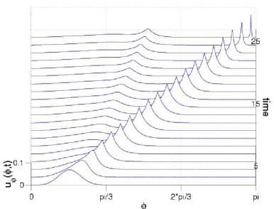
Figure 1: An initial Gaussian breaks up into Puckons, two of which are evident for the times shown.

As time elapses ($t=0$ is at the bottom of the figure, and later times are shown above it), a Puckon emerges from the Gaussian in Figure 1, and a second Puckon begins to emerge. In agreement with the prediction of equation (24), the first Puckon retains its height (and thus retains its velocity and canonical momentum $P$) as it approaches the South Pole.

A rear-end collision between two irrotational Puckons is shown in Figure 2.

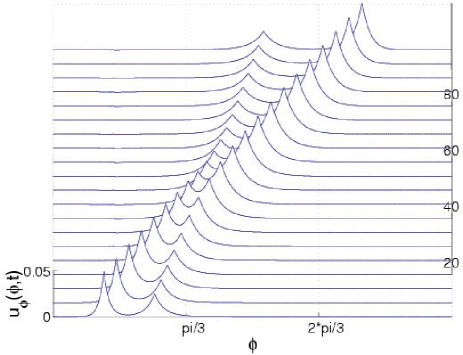
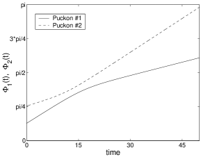
Figure 2: Two Puckons undergo a rear-end collision. The PDE simulation agrees with the colatitudes $\Phi$ of the ODE simulation to within 1% and with the canonical momenta $P$ to within 3%.

As the plot of colatitudes shows, these two Puckons do not pass through each other. Instead, they bounce and exchange momenta. However, their momenta are not exchanged exactly, as the plot of $P(t)$ shows. This contrasts with 2-soliton collisions for completely integrable PDEs in which momentum is exactly exchanged.

A head-on collision between two irrotational Puckons is shown in Figure 3.

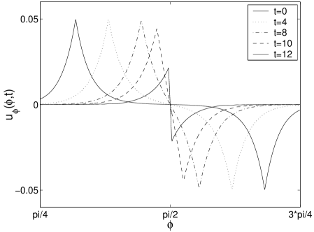
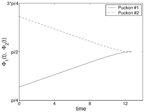
Figure 3: Two Puckons undergo a head-on collision.

In the PDE simulation, a vertical slope appears to form in finite time. Note that the Puckon velocities (i.e., the Puckon heights in the PDE simulation or the slopes of $\Phi(t)$ in the ODE simulation) remain finite and actually decrease to zero, whereas the equal and opposite canonical radial Puckon momenta diverge as the collision takes place.

Rotating Puckons.

Now we consider rotating Puckons ($u_{\theta}\neq 0$). Figure 4 shows the PDE evolution when the initial meridional velocity $u_{\phi}$ is zero and the initial azimuthal velocity $u_{\theta}$ is a Gaussian.

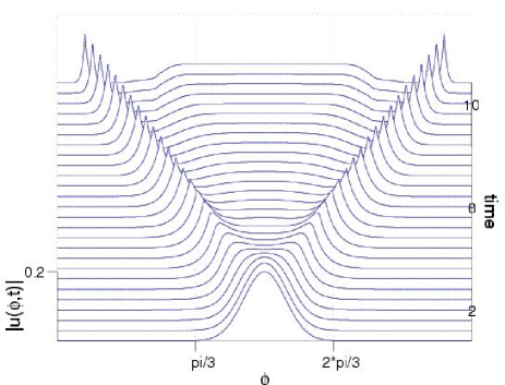
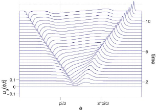
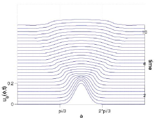
Figure 4: The evolution when the initial meridional velocity $u_{\phi}$ is zero and the initial azimuthal velocity $u_{\theta}$ is a Gaussian. The larger picture shows the magnitude of the velocity. Two rotating Puckons have emerged at the time shown, and two more are in the process of emerging from the Gaussian.

Two rotating Puckons have emerged from the Gaussian by the time shown, and they are moving toward opposite poles. The Puckons each have small but nonzero azimuthal velocities.

Finally, Figure 5 shows an ODE simulation of a single rotating Puckon when the length scale is $\alpha=1$ and the canonical variables are initially $\Phi=1.5$, $P=-1$, $M=-2$.

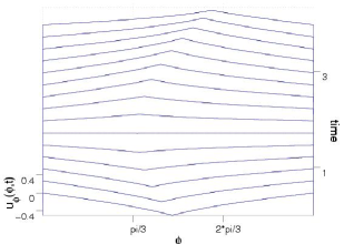
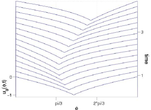
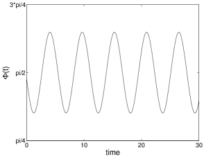
Figure 5: A single rotating Puckon for length scale $\alpha=1$. The initial parameters are $\Phi=1.5$, $P=-1$, $M=-2$. The PDE simulation shows about half of a period of the Puckon’s motion, and the ODE simulation shows about five periods of the Puckon’s motion. The meridional and azimuthal velocity components $u_{\phi}$ and $u_{\theta}$ are shown for the PDE simulation.

As discussed in Subsection 3.4, the basic rotating Puckon moves between minimum and maximum colatitudes. The Puckon is initially moving toward the North Pole, and one can see that its meridional velocity vanishes as it changes its direction and moves toward the South Pole. Its azimuthal velocity is negative throughout, i.e., it does not change its sense of rotation. Numerically, the Puckon moves between minimum and maximum colatitudes of (to five significant digits) 1.1033 and 2.0384, in comparison with the corresponding values of 1.1031 and 2.0385 predicted by the formula given in Subsection 3.4. Also, the numerical result for the period of the Puckon’s motion (averaged over the first five periods) agrees to six significant digits (5.60858) with the value given in Subsection 3.4. Thus, these numerical results for the ODE dynamics are accurate to between four and six significant figures.

5 Generalising to Other Surfaces

We now wish to extend these Hamiltonian reductions for diffeons on the sphere to other surfaces. For the moment, we retain the rotational symmetry.

5.1 Rotationally Symmetric Surfaces

Any surface $\Sigma$ with an isometric action of ${\mathrm{S}^{1}}$ has rotationally invariant coordinate charts on which the metric is given by

$$g=\mathrm{d}r^{2}+\psi(r)^{2}\mathrm{d}\theta^{2}$$

where $(r,\theta)\in(r_{min},r_{max})\times(0,2\pi)$. We may take $r_{min}=0$ to describe a fixed point of the motion. Let $\nabla$ be the Levi-Civita connection with respect to this metric and set

$$\mathbb{I}=(\,{\mathrm{l}\!\!\!{1}}+\Delta^{\nabla}).$$

By the Bochner-Wietzenböck theorem on 1-forms we compute

$$\mathbb{I} = \,{\mathrm{l}\!\!\!{1}}+\Delta^{d}-\mathrm{Ric}$$

$$= \left(\frac{\psi+\psi^{\prime\prime}}{\psi}\right)\,{\mathrm{l}\!\!\!{1}}+\Delta^{\mathrm{d}}.$$

We also have the explicit relation,

$$\Delta^{\mathrm{d}}(a(r)\mathrm{d}r+b(r)\mathrm{d}\theta)=-\frac{\partial}{\partial{r}}\left(\frac{1}{\psi}\frac{\partial}{\partial{r}}(\psi a(r))\right){\mathrm{d}{r}}-\psi\frac{\partial}{\partial{r}}\left(\frac{1}{\psi}\frac{\partial}{\partial{r}}(b(r))\right)\mathrm{d}\theta.$$

Suppose that $u$ is a rotationally invariant vector field on $\Sigma$. That is, suppose

$${\mbox{\boldmath$u$}}=u^{r}(r)\partial_{r}+u^{\theta}(r)\partial_{\theta}\,,$$

then the singular momentum solution ansatz for EPDiff,

$$\mathbb{I}{\mbox{\boldmath$u$}}_{\flat}=\frac{\delta(r-R)}{\psi(R)}\mathrm{d}r+\psi(R)\delta(r-R)\mathrm{d}\theta\,,$$ (32)

is a system of ordinary differential equations in $r$. We may solve this system to obtain two rotationally invariant, continuous functions $G^{r},G^{\theta}$ of $r$ and $R$, within our coordinate chart, which are symmetric in the two variables and which satisfy

$$\mathbb{I}\left(G^{r}(r,R)\mathrm{d}r+G^{\theta}(r,R)\mathrm{d}\theta\right)=\frac{\delta(r-R)}{\psi(R)}\mathrm{d}r+\psi(R)\delta(r-R)\mathrm{d}\theta\,.$$

The two Green’s functions $G^{r},G^{\theta}$ are related by

$$G^{\theta}(r,R)=\psi(r)\psi(R)G^{r}(r,R).$$

They also have a jump in the derivative along the diagonal $r=R$. Thus the solution of (32) for the velocity $u$ is

$$u = \left(G^{r}(r,R)\mathrm{d}r+\psi(r)\psi(R)G^{r}(r,R)\mathrm{d}\theta\right)^{\sharp}$$

$$= {G^{r}(r,R)}\frac{\partial}{\partial{r}}+\psi(R)\frac{G^{r}(r,R)}{\psi(r)}\frac{\partial}{\partial{\theta}}\,.$$

The EPDiff equations on the rotationally symmetric surface $\Sigma$ are

$$m = \mathbb{I}{\mbox{\boldmath$u$}}_{\flat}=\sum_{i=1}^{N}\frac{\delta(r-R_{i})}{\psi(R_{i})}\left(P_{i}\mathrm{d}r+M_{i}\mathrm{d}\theta\right)$$ (33)

$$0 = \frac{\partial{{\mbox{\boldmath$m$}}}}{\partial{t}}+\mathrm{ad}_{{\mbox{\boldmath$u$}}}^{*}{\mbox{\boldmath$m$}}\,,$$ (34)

and these equations extremise

$$\ell[{\mbox{\boldmath$u$}}] = \frac{1}{2}\int_{\Sigma}(|{\mbox{\boldmath$u$}}|_{g}^{2}+|\nabla{\mbox{\boldmath$u$}}|_{g}^{2})\mathrm{d}vol_{g}$$

$$= \frac{1}{2}\int_{\Sigma}\left\langle{\mbox{\boldmath$u$}},\mathbb{I}{\mbox{\boldmath$u$}}\right\rangle\mathrm{d}vol_{g}$$

$$= \frac{1}{2}\int_{\Sigma}{\mbox{\boldmath$m$}}({\mbox{\boldmath$u$}})\mathrm{d}vol_{g}\,.$$

After the Legendre transformation we arrive at the Hamiltonian

$$H[{\mbox{\boldmath$m$}}] = \int_{\Sigma}{\mbox{\boldmath$m$}}({\mbox{\boldmath$u$}})\mathrm{d}vol-\ell[{\mbox{\boldmath$u$}}]$$

$$= \frac{1}{2}\int_{\Sigma}{\mbox{\boldmath$m$}}({\mbox{\boldmath$u$}})\mathrm{d}vol.$$

We already know that the solution to (33) is

$${\mbox{\boldmath$u$}}_{\flat}=\sum_{i=1}^{N}\frac{G^{r}(r,R_{i})}{\psi(R_{i})}\Big{(}P_{i}\psi(R_{i})\mathrm{d}r+{M_{i}}\psi(r)\mathrm{d}\theta\Big{)},$$

that is,

$$u = \sum_{i=1}^{N}\frac{G^{r}(r,R_{i})}{\psi(r)\psi(R_{i})}\left(P_{i}\psi(R_{i})\psi(r)\frac{\partial}{\partial{r}}+{M_{i}}\frac{\partial}{\partial{\theta}}\right)$$

$$=: u_{r}\frac{\partial}{\partial{r}}+u_{\theta}\frac{\partial}{\partial{\theta}}\,.$$

Because $m$ is only supported within our coordinate chart and is invariant under the action of ${\mathrm{S}^{1}}$, we have

$$H({\mbox{\boldmath$m$}})=\frac{1}{2}2\pi\sum_{i=1}^{N}\left(P_{i}u_{r}(R_{i})+M_{i}u_{\theta}(R_{i})\right)$$

where $2\pi$ arises as the volume of ${\mathrm{S}^{1}}$. Choose a vector field $w=f(r,\theta)\frac{\partial}{\partial{r}}+g(r,\theta)\frac{\partial}{\partial{\theta}}$. Again since $m$ is supported within our chart, we know that

$$\int_{\sigma}{\mbox{\boldmath$m$}}(w)\mathrm{d}vol_{g}=\sum_{i}\int_{0}^{2\pi}\left(P_{i}f(R_{i},\theta)+M_{i}g(R_{i},\theta)\right)\mathrm{d}\theta.$$

We also have

$$\left[w,{\mbox{\boldmath$u$}}\right]=\left(fu_{r}^{\prime}-u_{r}\partial_{r}f-u_{\theta}\partial_{\theta}f\right)\frac{\partial}{\partial{r}}+\left(fu_{\theta}^{\prime}-u_{r}\partial_{r}g-u_{\theta}\partial_{\theta}g\right)\frac{\partial}{\partial{\theta}}.$$

Consequently, the EPDiff equations yield

$$0 = \int_{\Sigma}\left(\frac{\partial}{\partial{t}}({\mbox{\boldmath$m$}}(w))+{\mbox{\boldmath$m$}}([w,{\mbox{\boldmath$u$}}])\right)\mathrm{d}vol_{g}$$

$$= \int_{0}^{2\pi}\frac{\partial}{\partial{t}}\left(P_{i}f(R_{i},\theta)+M_{i}g(R_{i},\theta)\right)\mathrm{d}\theta$$

$$+ \int_{0}^{2\pi}\left(P_{i}\left(fu_{r}^{\prime}-u_{r}\partial_{r}f-u_{\theta}\partial_{\theta}f\right)+M_{i}\left(fu_{\theta}^{\prime}-u_{r}\partial_{r}g-u_{\theta}\partial_{\theta}g\right)\right)\big{|}_{r=R_{i}}\mathrm{d}\theta$$

$$= \int_{0}^{2\pi}\left(\dot{P}_{i}f(R_{i},\theta)+P_{i}\dot{R}_{i}\partial_{r}f(R_{i},\theta)+\dot{M}_{i}g(R_{i},\theta)+M_{i}\dot{R_{i}}\partial_{r}g(R_{i},\theta)\right)\mathrm{d}\theta$$

$$+ \int_{0}^{2\pi}\left(P_{i}\left(fu_{r}^{\prime}-u_{r}\partial_{r}f\right)+M_{i}\left(fu_{\theta}^{\prime}-u_{r}\partial_{r}g\right)\right)\big{|}_{r=R_{i}}\mathrm{d}\theta.$$

Comparing coefficients of $f,\partial_{r}f,g\partial_{r}g$ now yields

$$0 = \dot{P}_{i}+P_{i}u_{r}^{\prime}(R_{i})+M_{i}u_{\theta}^{\prime}(R_{i})$$

$$0 = P_{i}\dot{R}_{i}-P_{i}u_{r}(R_{i})$$

$$0 = \dot{M}_{i}$$

$$0 = M_{i}\dot{R}_{i}-M_{i}u_{r}(R_{i})$$

Now since

$$u_{r}(R_{i})=\sum_{j=1}^{N}G^{r}(R_{i},R_{j})$$

and

$$u_{r}^{\prime}(R_{i})=\sum_{j=1}^{N}\frac{\partial{G^{r}}}{\partial{r}}(R_{i},R_{j})$$

we see that

$$\frac{\partial}{\partial{R_{i}}}\sum_{j=1}^{N}u_{r}(R_{j}) = \frac{\partial}{\partial{R_{i}}}\sum_{j,k=1}^{N}G^{r}(R_{j},R_{k})$$

$$= \sum_{j,k=1}^{N}\left(\frac{\partial{R_{j}}}{\partial{R_{i}}}\left.\frac{\partial{G^{r}(r,R)}}{\partial{r}}\right|_{r=R_{j},R=R_{k}}+\frac{\partial{R_{k}}}{\partial{R_{i}}}\left.\frac{\partial{G^{r}(r,R)}}{\partial{R}}\right|_{r=R_{j},R=R_{k}}\right)$$

$$= \sum_{j,k=1}^{N}\left(\frac{\partial{R_{j}}}{\partial{R_{i}}}\left.\frac{\partial{G^{r}(r,R)}}{\partial{r}}\right|_{r=R_{j},R=R_{k}}+\frac{\partial{R_{k}}}{\partial{R_{i}}}\left.\frac{\partial{G^{r}(r,R)}}{\partial{r}}\right|_{r=R_{k},R=R_{j}}\right)$$

$$\hbox{since }G^{r}\hbox{ is symmetric in its arguments}$$

$$= \sum_{j,k=1}^{N}\left(\delta_{ij}\left.\frac{\partial{G^{r}(r,R)}}{\partial{r}}\right|_{r=R_{j},R=R_{k}}+\delta_{ki}\left.\frac{\partial{G^{r}(r,R)}}{\partial{r}}\right|_{r=R_{k},R=R_{j}}\right)$$

$$= \sum_{k=1}^{N}\left.\frac{\partial{G^{r}(r,R)}}{\partial{r}}\right|_{r=R_{i},R=R_{k}}+\sum_{j=1}^{N}\left.\frac{\partial{G^{r}(r,R)}}{\partial{r}}\right|_{r=R_{i},R=R_{j}}$$

$$= 2\sum_{j=1}^{N}\left.\frac{\partial{G^{r}(r,R)}}{\partial{r}}\right|_{r=R_{i},R=R_{j}}$$

$$= 2u_{r}^{\prime}(R_{i}).$$

Similarly

$$u_{\theta}^{\prime}(R_{i})=\frac{1}{2}\frac{\partial}{\partial{R_{i}}}\sum_{j=1}^{N}u_{\theta}(R_{j}).$$

This finally yields

$$\dot{P}_{i} = -\frac{1}{2}\frac{\partial}{\partial{R_{i}}}\sum_{j=1}^{N}\left(P_{j}u_{r}(R_{j})+M_{j}u_{\theta}(R_{j})\right)$$ (35)

$$\dot{R}_{i} = u_{r}(R_{i})$$ (36)

$$\dot{M}_{i} = 0.$$ (37)

Thus, we have proved the following realisation of the momentum map in [5].

Proposition 5.1 (Canonical equations for rotationally symmetric diffeons)

The parameters $P_{i},R_{i}$ for diffeons on a rotationally symmetric surface $\Sigma$ with constant positive curvature and metric given by $g=\mathrm{d}r^{2}+\psi(r)^{2}\mathrm{d}\theta^{2}$ satisfy Hamilton’s canonical equations with Hamiltonian given by

$$H(\mathbf{P},\mathbf{R};\mathbf{M}) = \frac{1}{2\pi}\left(\int_{\Sigma}{\mbox{\boldmath$m$}}({\mbox{\boldmath$u$}})\mathrm{d}vol-\ell[{\mbox{\boldmath$u$}}]\right)$$

$$= \frac{1}{2}\sum_{i=1}^{N}\left(P_{i}u_{r}(R_{i})+M_{i}u_{\theta}(R_{i})\right)$$

$$= \frac{1}{2}\sum_{i,j=1}^{N}\frac{G^{r}(R_{i},R_{j})}{\psi(R_{i})\psi(R_{j})}\left(P_{i}P_{j}\psi(R_{i})\psi(R_{j})+M_{i}M_{j}\right).$$

A solution to (35,36,37) is an example of an $N$-diffeon on a rotationally symmetric surface $\Sigma$.

We notice that the critical points of $H$ are those $\mathbf{R}=(R_{1},...,R_{n})$ such that $G^{r}(R_{i},R_{j})=0$ for all $i,j$. But the value of $H$ at these critical points is always $0$ since $H$ depends on $G^{r}$.

Remark 5.2

The only 1-dimensional Lie Groups are $\mathbb{R}$ and ${\mathrm{S}^{1}}$, and while we have considered the isometric action of ${\mathrm{S}^{1}}$ on a surface, we have to be more careful with translation invariance because the group ceases to be compact. However we can consider $\theta$, which parameterises each orbit $r=const$, taking values in $(-L,L)$ rather than $(-\infty,\infty)$ for the full translation group. This makes the integration finite.

5.2 Rotationally Invariant Diffeons on Hyperbolic Space

Hyperbolic space has a richer structure than either the plane, or the sphere. Indeed, the isometry group of the sphere is ${\mathrm{SO}}(3)$; so all isometries are rotations. We have already examined the case of rotationally invariant diffeons. (These are the Puckons.) The isometry group of the plane $\mathbb{R}^{2}$ is ${\mathrm{S}^{1}}\ltimes\mathbb{R}^{2}$, the semi-direct product of rotations and translations. Translational invariance yields the direct product of the original 1-dimensional peakons, whereas rotational invariance yields the rotating circular peakons developed in [8]. However, the isometry group of hyperbolic space is $\mathbb{P}{\mathrm{SL}}(2,\mathbb{R})$, which is not compact and contains three different types of isometry. These are the rotational, translational and horolational subgroups.

The Hamiltonian for hyperbolic $N$-diffeons with rotational symmetry.

We have already done most of the work for the rotationally symmetric case. All that remains is to write the hyperbolic metric in a conformally flat way and from it deduce the Green’s functions $G^{r}$ and $G^{\theta}$. The model is familiar: we use the Poincaré disc $D=\{(x,y)\in\mathbb{R}^{2}|\ x^{2}+y^{2}<1\}$ in polar coordinates with the metric

$$g_{\mathcal{H}}=\frac{4}{(1-r^{2})^{2}}\left({\mathrm{d}{r}}^{2}+r^{2}\mathrm{d}\theta^{2}\right),$$

i.e. the conformal parameter is

$$\rho(r)=\frac{2}{1-r^{2}}\,.$$

The Bochner-Wietzenböck formula states that on $\mathrm{T}{D}$

$$\Delta^{\mathrm{d}}=\Delta^{\nabla}-\,{\mathrm{l}\!\!\!{1}}\,,$$

so that

$$\mathbb{I}=\,{\mathrm{l}\!\!\!{1}}+\Delta^{\nabla}=2\,{\mathrm{l}\!\!\!{1}}+\Delta^{\mathrm{d}}.$$ (38)

We wish to find Green’s functions $G^{r}$ and $G^{\theta}$ such that

$$\mathbb{I}(G^{r}(r,R){\mathrm{d}{r}}+G^{\theta}(r,R)\mathrm{d}\theta)=\delta(r-R)\left(\frac{1}{R}{\mathrm{d}{r}}+R\mathrm{d}\theta\right).$$

We also ask that these Green’s functions be finite at the origin, continuous and symmetric in their variables. Explicitly, we have

$$\Delta^{\mathrm{d}}\left(a(r){\mathrm{d}{r}}+b(r)\mathrm{d}\theta\right)=-\frac{\partial}{\partial{r}}\left(\frac{1}{\rho^{2}r}\frac{\partial}{\partial{r}}(ra(r))\right){\mathrm{d}{r}}-r\frac{\partial}{\partial{r}}\left(\frac{1}{\rho^{2}r}\frac{\partial{b}}{\partial{r}}\right)\mathrm{d}\theta.$$

Upon setting

$$F(r)=2-2r^{4}+8\log(r)r^{2}+r^{2}$$

we write

$$G^{r}(r,R)=\frac{\rho(r)^{2}\rho(R)^{2}}{16}\frac{\min(r,R)}{\min(r,R)}F(\max(r,R)),$$

and hence

$$G^{\theta}(r,R)=RrG^{r}(r,R).$$

Thus, we have shown the following.

Proposition 5.3 (Hamiltonian for rotationally invariant hyperbolic $N$-diffeons)

The Hamiltonian for rotationally invariant $N$-diffeons on hyperbolic space is given by

$$H(\mathbf{P},\mathbf{R};\mathbf{M}) = \frac{1}{2}\sum_{i,j=1}^{N}\frac{1}{\rho(R_{i})^{2}R_{i}\rho(R_{j})^{2}R_{j}}\left(P_{i}P_{j}R_{i}R_{j}G^{r}(R_{i},R_{j})+\frac{M_{i}M_{j}}{R_{i}R_{j}}G^{\theta}(R_{i},R_{j})\right)$$

$$= \frac{1}{2}\sum_{i,j=1}^{N}\frac{G^{r}(R_{i},R_{j})}{\rho(R_{i})^{2}R_{i}\rho(R_{j})^{2}R_{j}}\left(P_{i}P_{j}R_{i}R_{j}+M_{i}M_{j}\right).$$

The hyperbolic diffeon.

Let us examine the behaviour of the basic rotationally symmetric hyperbolic diffeon. The Hamiltonian is

$$H(P,R) = \frac{1}{2}\frac{G^{r}(R,R)}{\rho(R)^{4}R^{2}}\left(P^{2}R^{2}+{M^{2}}\right)$$

$$= \frac{F(R)}{32R^{2}}\left(P^{2}R^{2}+{M^{2}}\right).$$

The function $F(R)/R^{2}$ is positive and continuous on $(0,1)$, and it has a singularity at $R=0$. Its derivative is negative on $(0,1)$ and its image is $(1,\infty)$. Consequently, $F(R)/R^{2}$ is an invertible function $(0,1)\longrightarrow(1,\infty)$.

Assuming $M\neq 0$, on the level set $H(P,R)=K^{2}$ we find that

$$P^{2}=\frac{32K^{2}}{F(R)}-\frac{M^{2}}{R^{2}}\,.$$

So $\dot{R}=0$, whenever

$$\frac{F(R)}{R^{2}}=\frac{32K^{2}}{M^{2}}.$$

Hence, whenever $32K^{2}>M^{2}>0$, precisely one turning point exists for $R$. This proves the following.

Proposition 5.4

Rotating diffeons with $M^{2}>0$ on a rotationally symmetric hyperbolic surface do not exhibit periodic behaviour.

For the irrotational diffeon, $M=0$ and we have

$$P^{2}=\frac{32K^{2}}{F(R)}\,.$$

Since $F(R)>0$ for all $R\in[0,1]$, the irrotational diffeon has no turning points of $R$ at all.

5.3 Horolationally Invariant Diffeons on Hyperbolic Space

We now turn to a subtly different problem. So far we have been using solely the rotation group (the circle) to produce symmetric diffeons. Now we consider a different subgroup of hyperbolic isometries. This time it is expedient to use the upper-half-plane model of hyperbolic geometry. That is,

$$\mathcal{H}=\{(x,y)\in\mathbb{R}^{2}|y>0\}$$

with the metric

$$g_{\mathcal{H}}=\frac{\mathrm{d}x^{2}+\mathrm{d}y^{2}}{y^{2}}\,.$$

The group we consider is the horolation group $(x,y)\mapsto(x+a,y)$. This is a unique type of isometry in planar geometries and is, figuratively speaking, a “rotation about infinity”. We can see immediately that the orbits of this group action are the lines $y=const$, and that we seek diffeons which are independent of $x$. In this situation by (38),

$$\mathbb{I}(a(y)\mathrm{d}x+b(y)\mathrm{d}y)=\frac{1}{y}\left(2ya-\frac{\partial{{}^{2}a}}{\partial{y^{2}}}y^{3}-2\frac{\partial{a}}{\partial{y}}y^{2}\right)\mathrm{d}x+\left(2b-\frac{\partial{{}^{2}b}}{\partial{y^{2}}}y^{2}-2\frac{\partial{b}}{\partial{y}}y\right)\mathrm{d}y$$

Thus the solution to

$$\mathbb{I}(G(y,Y)\mathrm{d}x)=\delta(y-Y)\mathrm{d}x$$

is

$$G(y,Y)=\frac{\min(y,Y)}{3\max(y,Y)^{2}},$$

and this solution also solves

$$\mathbb{I}(G(y,Y)\mathrm{d}y)=\delta(y-Y)\mathrm{d}y.$$

Next, we consider the compactness issue. Since the coordinate $x$ ranges from $-\infty$ to $\infty$ we know that functions that only involve $y$ cannot be integrated across all of $\mathcal{H}$. Thus the Diffeon Hamiltonian cannot exist over the whole space and the theory of section 5.1 does not apply. Let us restrict ourselves to the strip $B_{L}=\{(x,y)|y>0,|x|<L\}\subset\mathcal{H}$. By doing this we can apply similar calculations to those used in section 5.1 to $B_{L}$, but we must apply them only in the case of vector fields which are tangent to the boundary $x=\pm L$.

Thus if

$${\mbox{\boldmath$m$}}=\sum_{i=1}^{N}\delta(y-Y_{i})Y_{i}^{2}(M_{i}\mathrm{d}x+P_{i}\mathrm{d}y)$$

then we arrive at the Hamiltonian

$$H(\mathbf{P},\mathbf{Y}) = L\sum_{i,j=1}^{N}G(Y_{i},Y_{j})Y_{i}^{2}Y_{j}^{2}(P_{i}P_{j}+M_{i}M_{j})$$

$$= L\sum_{i,j=1}^{N}\frac{\min(Y_{i},Y_{j})}{3\max(Y_{i},Y_{j})^{2}}Y_{i}^{2}Y_{j}^{2}(P_{i}P_{j}+M_{i}M_{j})$$

$$= L\sum_{i,j=1}^{N}\frac{\min(Y_{i},Y_{j})^{3}}{3}(P_{i}P_{j}+M_{i}M_{j})$$

and the condition that $\dot{M}_{i}=0$.

For the 1-diffeon, the Hamiltonian is

$$H(P,Y)=L\frac{Y^{3}}{3}(P^{2}+M^{2})$$

so for $H(P,Y)=const=K$, the only turning point of $Y$ is at

$$Y=\sqrt[3]{\frac{3K}{LM^{2}}}$$

or at 0, if $M=0$.

Remark 5.5

Joining the edges of $B_{L}$ together yields a surface called Gabriel’s Horn, whereby the translation invariant diffeons on $B_{L}$ become rotationally invariant diffeons on Gabriel’s horn.

5.4 Translation Invariant Diffeons on Hyperbolic Space

Translations on the Hyperbolic plane are characterised by having two ideal fixed points. The version of the metric we use in this case for the upper half plane is

$$g_{\mathcal{H}}=\mathrm{d}r+\cosh^{2}r\mathrm{d}\theta^{2}\,,$$

where the subsets formed by $r=const$ are the orbits of the translation. Again, the orbits are not compact, so we limit ourselves to the strip $B_{L}=\{(r,\theta)\in\mathbb{R}^{2}|r>0,|\theta|<L\}\subset\mathcal{H}$.

In this situation, the Green’s function $G(r,R)$ solving

$$\mathbb{I}G(r,R)\mathrm{d}r=\frac{\delta(r-R)}{\cosh(R)}\mathrm{d}r$$

is given by

$$G(r,R)=\frac{1}{2}\tanh(\min(r,R))\cosh(\max(r,R))+\cosh(r)\cosh(R)\arctan(e^{\min(r,R)}).$$

Due to the complicated form of the Green’s function, we will not write down the explicit form of the Hamiltonian for the $N$-diffeon. However, the Hamiltonian for the 1-diffeon is,

$$H(P,R;M) = \frac{1}{2}\frac{G(R,R)}{\cosh^{2}R}\left(P^{2}\cosh^{2}R+M^{2}\right)$$

$$= \frac{1}{4}\left(\tanh R\,\mathrm{sech}\,R+2\arctan(e^{R})\right)\left(P^{2}\cosh^{2}R+M^{2}\right).$$

In this case

$$\frac{\partial{H}}{\partial{P}} = \frac{1}{2}\left(\tanh R\,\mathrm{sech}\,R+2\arctan(e^{R})\right)P\cosh^{2}R\,,$$

$$\frac{\partial{H}}{\partial{R}} = \frac{1}{2}\left(P^{2}\left(\cosh{R}+\sinh{2R}\arctan(e^{R})\right)+M^{2}\,\mathrm{sech}^{3}\,R\right)\,.$$

It can be shown that there are no equilibria for the motion unless $M=0$, where the line $P=0$ is the critical point set for $H$. However,

$$H(0,R)=0\,,$$

for each value of $R$. So the line $P$ consists entirely of stationary points, and since away from this line no points exist for which $\dot{R}=0$, there can be no periodic behaviour of 1-diffeons in this case.

Extending EPDiff on Hyperbolic Space

Our study of EPDiff on hyperbolic spaces so far shows that the behaviour of hyperbolic diffeons seems less interesting than the rich dynamical structure of multiple Puckons interacting on the sphere. This is because hyperbolic diffeons will bounce only once before heading off to infinity, in the cases we have studied so far.

However, hyperbolic space is related intimately with the study of curves of genus at least 2: it forms the universal cover for all such Riemann surfaces. So far, we have been unable to examine the case of curves of genus $\geq 2$ simply because their isometry groups are so small (usually discrete) that we simply cannot find a 1-parameter subgroup by which we may reduce the EPDiff equations to ODEs.

Any high genus Riemann surface can be realised as the quotient of the hyperbolic plane by a tiling, or hyperbolic lattice [17]. The complex structure of the Riemann surface depends upon the shape of the lattice. A surface $\Sigma$ of genus $\gamma\geq 2$ is determined topologically by the symmetry group of the tiling; but there are a variety of complex structures which may be put upon $\Sigma$ to turn it into a Riemann Surface. If $\Gamma$ is the symmetry group of the tiling, then the space of complex structures which may be put on $\Sigma$ is given by the space

$$T_{\Gamma}=\frac{\Gamma\hbox{-invariant quasiconformal maps of }\mathbb{D}}{\hbox{Hyperbolic isometries of }\mathbb{D}}.$$

Here $\mathbb{D}$ is the Poincaré disc (the unit disc in the complex plane). In the space $T_{\Gamma}$ a quasiconformal map is a generalisation of a conformal map in which although angles are not preserved, the angular dilation is uniformly bounded, see [1, 4].

The inclusion of a subgroup $\Gamma^{\prime}$ in $\Gamma$ induces a natural inclusion of $T_{\Gamma}$ in $T_{\Gamma^{\prime}}$, so it makes sense to consider the universal Teichmüller space as the Teichmüller space $T_{1}$ associated with the trivial group. The universal Teichmüller space is endowed with the Weil-Petersson metric, thus providing the framework essential for the theory of EPDiff. Furthermore, the restriction of the maps given in the definition of Teichmüller space to the boundary of the disc provides us with the essential method by which we reduce the EPDiff PDEs to ODEs. This study is beyond the scope of this paper and we present the results in the next, [7].

6 EPDiff on Higher Dimensional Manifolds with Symmetry

Our calculation for surfaces in the previous sections impose a rotational symmetry of the solutions. That is, the solutions are invariant under a circle action, and this effectively reduces $\mathbb{I}$ in (38) to an ordinary differential operator. As a result, we are able to find $G^{r}$ and $G^{\theta}$ which are invariant under the group action, continuous and have a jump in the derivative along an orbit. This motivates the study of higher dimensional Riemannian manifolds $(\Sigma,g)$ which possess an isometric action of the Lie group $G$ such that the quotient space $\Sigma/G$ is a 1-dimensional orbifold.

6.1 Principal Bundles over 1-Dimensional Manifolds

We consider first the case of principal bundles over 1-dimensional manifolds. It is a well known fact that 1-manifolds are diffeomorphic to $\mathbb{R}$, $[0,\infty)$, $[0,1]$ or ${\mathrm{S}^{1}}$, see for example pp55-57 of [13]. Intervals of $\mathbb{R}$ are all contractible, we know that any principal bundle over them is trivial. The principal $K$-bundles of ${\mathrm{S}^{1}}$ are up to isomorphism in 1-1 correspondence with $\pi_{1}(BK)$, the fundamental group of the classifying space $BK$ of the Lie group $K$. However, by the long exact sequence of homotopy groups (see [11]), we know that $\pi_{1}(BK)\cong\pi_{0}(K)$, thus if $K$ is connected, then any Principal $K$-bundle over ${\mathrm{S}^{1}}$ is trivial.

The upshot here is that if $\Sigma$ is a Riemannian manifold with a free isometric action of $K$ and $\Sigma/K$ is a 1-dimensional manifold $N$, then $\Sigma\cong K\times N$.

6.2 Warped Products

Let $K$ be a compact semi-simple Lie group of dimension $n-1$ and $\Sigma\longrightarrow I\subset\mathbb{R}$ a principal $K$-bundle over the open interval $I$ (in fact in what follows, we may also take $I$ to be the circle ${\mathrm{S}^{1}}$). Suppose $\Sigma$ has a Riemannian metric $g$ preserved by $K$, and that coordinates exist such that the metric has the form of a warped product

$$g=\mathrm{d}r^{2}+\psi(r)^{2}g_{K}$$

where $g_{K}$ is a bi-invariant inner product on $\mathrm{T}{K}$ and $\psi$ is a $K$-invariant function on $\Sigma$, i.e. a function of $r$ alone. The coordinate $r$ parameterises the orbit of $K$ in $\Sigma$. Let $\nabla$ be the Levi-Civita connection with respect to $g$.

This situation is rich enough to produce interesting results. In what follows $\{\xi_{i}\}_{i=1}^{n}$ will be a $g_{K}$ orthonormal basis of $\mathfrak{k}$ and $X_{\xi}$ the left-invariant vector field generated by $\xi\in\mathfrak{k}$. We write $X_{i}=X_{\xi_{i}}$, these form an orthonormal frame of $\mathrm{T}{K}$; set $\theta^{i}$ to be the coframe dual to the $X_{i}$ . Let $\nabla^{K}$ be the Levi-Civita connection of $K$ with respect to $g_{K}$.

Proposition 6.1

We have

$$\Delta^{\nabla^{K}}X_{i}=kX_{i}.$$

This follows from the identity on $K$,

$$\nabla_{X_{i}}^{K}X_{j}=\frac{1}{2}[X_{i},X_{j}]\,.$$

Thus, $\Delta^{\nabla^{K}}$ will be the Casimir operator associated with the adjoint representation of $K$ on $\mathfrak{k}$ applied to the frame $\{X_{i}\}$. The Casimir however is just a constant multiple of the identity, the constant $k$ being

$$k=1-\frac{\dim\mathfrak{z}(K)}{\dim\mathfrak{k}}$$

where $\mathfrak{z}(K)$ is the Lie algebra of centre of the group $K$.

The geometry of warped products is reasonably well known, [2, 14]. As an exercise in Riemannian geometry, one may deduce (see pp58-59 of [2])

Proposition 6.2

Let $f$ be a $K$-invariant function on $\Sigma$ and suppose $\psi(r)=e^{\lambda(r)}$. The connection Laplacian associated with $g$ satisfies

$$\Delta^{\nabla}f{\mathrm{d}{r}} = -\left(\frac{\partial{{}^{2}f}}{\partial{r^{2}}}+(n-1)\frac{\partial{\lambda}}{\partial{r}}\frac{\partial{f}}{\partial{r}}-(n-1)\left(\frac{\partial{\lambda}}{\partial{r}}\right)^{2}f\right){\mathrm{d}{r}}$$

$$\Delta^{\nabla}fe^{\lambda}\theta^{i} = -\left(\frac{\partial{{}^{2}f}}{\partial{r^{2}}}+(n-1)\frac{\partial{\lambda}}{\partial{r}}\frac{\partial{f}}{\partial{r}}-\left(\frac{\partial{\lambda}}{\partial{r}}\right)^{2}f-e^{-\lambda}kf\right)e^{\lambda}\theta^{i}$$

These two propositions show us that the $K$-invariant equations

$$\mathbb{I}a^{0}(r){\mathrm{d}{r}} = \frac{\delta(r-R)}{\psi(R)}{\mathrm{d}{r}}$$ (39)

$$\mathbb{I}a^{i}(r)\psi(r)\theta^{i} = \delta(r-R)\theta^{i}$$ (40)

are $n$ ordinary differential equations in $r$. Thus, there are $n$ functions $G^{0}(r,R),G^{i}(r,R)$ that solve (39) and (40), respectively, are continuous on $r=R$, and are symmetric in the sense that

$$G^{0}(r,R) = G^{0}(R,r)$$

$${G^{i}(r,R)} = {G^{i}(R,r)}.$$

Indeed, the second identity in Proposition 6.2 shows that $G^{i}$ is independent of the index $i$. Hence, instead of $G^{i}$,we shall write $G^{K}$.

Now let $m$ be the measure-valued one-form

$${\mbox{\boldmath$m$}}^{j}=\sum_{i=1}^{N}\frac{\delta(r-R_{i})}{\psi(R_{i})}\left(P_{i}{\mathrm{d}{r}}+M_{i}\theta^{j}\right)$$ (41)

The solution to $\mathbb{I}({\mbox{\boldmath$u$}}_{j})_{\flat}={\mbox{\boldmath$m$}}^{j}$ is

$${\mbox{\boldmath$u$}}_{j} = \sum_{i=1}^{N}\left(P_{i}G^{0}(r,R_{i})\frac{\partial}{\partial{r}}+\frac{M_{i}}{\psi(r)\psi(R_{i})}G^{K}(r,R_{i})X_{j}\right)$$

$$= {u_{j}^{0}}(r)\frac{\partial}{\partial{r}}+u_{j}(r)X_{j}.$$

Note, we are not using the summation convention here. Also denote

$$w=f^{0}\frac{\partial}{\partial{r}}+f^{\zeta}X_{\zeta}$$

for any $\zeta\in\mathfrak{k}$. Any vector field on $\Sigma$ will be the sum of such vector fields $w$. Then we may write the vector field commutation relation,

$$[w,{\mbox{\boldmath$u$}}_{j}]=\left(f^{0}{u_{j}^{0}}^{\prime}-{u_{j}^{0}}\partial_{r}f^{0}-u_{j}X_{j}(f^{0})\right)\frac{\partial}{\partial{r}}-\left({u_{j}^{0}}\partial_{r}f^{\zeta}+u_{j}X_{j}(f^{\zeta})\right)X_{\zeta}+f^{0}u_{j}^{\prime}X_{j}.$$

Thus

$$\int_{\Sigma}{\mbox{\boldmath$m$}}^{j}(w)\mathrm{d}vol_{P} = \sum_{i=1}^{N}\int_{K}\int_{I}\frac{\delta(r-R_{i})}{\psi(R_{i})}\left(P_{i}f^{0}+M_{i}f^{\zeta}g_{K}(X_{\zeta},X_{j})\right)\psi(r){\mathrm{d}{r}}\mathrm{d}vol_{K}$$

$$= \sum_{i=1}^{N}\int_{h\in K}\left(P_{i}f^{0}(R_{i},h)+M_{i}f^{\zeta}(R_{i},h)\zeta^{j}\right)\mathrm{d}vol_{K}$$

where $\zeta=\sum_{l=1}^{n-1}\zeta^{j}\xi_{j}$. Especially, this yields the ad^∗ relation needed for expressing EPDiff in this setting,

$$\int_{\Sigma}{\mbox{\boldmath$m$}}^{j}([w,{\mbox{\boldmath$u$}}_{j}])$$

$$= \sum_{i=1}^{N}\int_{h\in K}P_{i}\left(f^{0}(R_{i},h){u_{j}^{0}}^{\prime}(R_{i})-{u_{j}^{0}}(R_{i})\partial_{r}f^{0}(R_{i},h)-u_{j}(R_{i})X_{j}(f^{0})(R_{i},h)\right)\mathrm{d}vol_{K}$$

$$- \sum_{i=1}^{N}\int_{h\in K}M_{i}\left({u_{j}^{0}}(R_{i})\partial_{r}f^{\zeta}(R_{i},h)\zeta^{j}+u_{j}X_{j}(f^{\zeta})(R_{i},h)\zeta^{j}-f^{0}(R_{i},h)u_{j}^{\prime}(R_{i})\right)\mathrm{d}vol_{K}\,.$$

Before we proceed, we note that while we were dealing with the circle, terms such as $u_{\theta}\partial_{\theta}f$ disappeared when we integrated over the circle, as one would expect from Stokes’ theorem. Here, however, we have the terms $u_{j}X_{j}(f^{0})$ and $u_{j}X_{j}(f^{\zeta})$. One asks, “Do these vanish when we integrate over the group $K$?” As w shall see, the answer to this question is, “Yes.”

From standard Riemannian geometry, one has

Proposition 6.3

For any compact Riemannian manifold $N$, and any vector field $X$ and function $\phi$ on $N$ we have

$$\int_{N}X(\phi)\mathrm{d}vol=\int_{N}\phi\,\mathrm{div}\,X\mathrm{d}vol\,.$$

From this formula we see that, in the present situation,

Proposition 6.4

Given any $\kappa\in\mathfrak{k}$ and any function $\phi$ on $K$.

$$\int_{K}X_{\kappa}(\phi)\mathrm{d}vol_{K}=0\,.$$

This relation follows because $X_{\kappa}$ generates volume preserving (metric preserving!) diffeomorphisms of $K$.

Hence, upon integrating over $K$, the terms $u_{j}X_{i}(f^{0})$ and $u_{j}X_{j}(f^{\zeta})$ will vanish because $u_{j}$ is $K$-invariant. Thus, we have

$$\int_{\Sigma}{\mbox{\boldmath$m$}}^{j}([w,{\mbox{\boldmath$u$}}_{j}]) = \sum_{i=1}^{N}\int_{h\in K}P_{i}\left(f^{0}(R_{i},h){u_{j}^{0}}^{\prime}(R_{i})-{u_{j}^{0}}(R_{i})\partial_{r}f^{0}(R_{i},h)\right)\mathrm{d}vol_{K}$$

$$- \sum_{i=1}^{N}\int_{h\in K}M_{i}\left({u_{j}^{0}}(R_{i})\partial_{r}f^{\zeta}(R_{i},h)\zeta^{j}-f^{0}(R_{i},h)u_{j}^{\prime}(R_{i})\right)\mathrm{d}vol_{K}$$

This formula implies the EPDiff equations,

$$0 = \int_{\Sigma}\left(\frac{\partial{{\mbox{\boldmath$m$}}^{j}}}{\partial{t}}(w)+{\mbox{\boldmath$m$}}^{j}([w,{\mbox{\boldmath$u$}}_{j}])\right)\mathrm{d}vol_{p}$$

$$= \sum_{i=1}^{N}\int_{h\in K}\left(\dot{P}_{i}f^{0}(R_{i},h)+P_{i}\dot{R}_{i}\frac{\partial}{\partial{R_{i}}}f^{0}(R_{i},h)+\dot{M}_{i}f^{\zeta}(R_{i},h)\zeta^{j}+M_{i}\dot{R}_{i}\frac{\partial}{\partial{R_{i}}}f^{\zeta}(R_{i},h)\zeta^{j}\right)\mathrm{d}vol_{K}$$

$$+ \sum_{i=1}^{N}\int_{h\in K}P_{i}\left(f^{0}(R_{i},h){u_{j}^{0}}^{\prime}(R_{i})-{u_{j}^{0}}(R_{i})\partial_{r}f^{0}(R_{i},h)\right)\mathrm{d}vol_{K}$$

$$- \sum_{i=1}^{N}\int_{h\in K}M_{i}\left({u_{j}^{0}}(R_{i})\partial_{r}f^{\zeta}(R_{i},h)\zeta^{j}-f^{0}(R_{i},h)u_{j}^{\prime}(R_{i})\right)\mathrm{d}vol_{K}$$

Again, we compare coefficients of $f^{0},f^{\zeta},\frac{\partial}{\partial{R_{i}}}f^{0}$ and $\frac{\partial}{\partial{R_{i}}}f^{\zeta}$ to find

$$0 = \dot{P}_{i}+P_{i}{u_{j}^{0}}^{\prime}(R_{i})+M_{i}u_{j}^{\prime}(R_{i})\,,$$

$$0 = P_{i}\dot{R}_{i}-P_{i}{u_{j}^{0}}(R_{i})\,,$$

$$0 = \dot{M}_{i}\zeta^{j}\,,$$

$$0 = M_{i}\dot{R}_{i}\zeta^{j}-M_{i}{u_{j}^{0}}(R_{i})\zeta^{j}\,.$$

Therefore, we have proven the following.

Theorem 6.5 (Hamiltonian diffeon reduction for $K$-invariant warped product spaces)

The warped product diffeon parameters in equation (41) satisfy

$$\dot{P}_{i} = -\,\frac{1}{2}\frac{\partial}{\partial{R_{i}}}\sum_{k=1}^{N}\left(P_{k}{u_{j}^{0}}(R_{k})+M_{k}u_{j}(R_{k})\right)\,,$$ (42)

$$\dot{R}_{i} = {u_{j}^{0}}(R_{i})\,,$$ (43)

$$\dot{M_{i}} = 0\,.$$ (44)

As guaranteed by the momentum map property of the diffeon solution ansatz (2) for EPDiff, these are Hamilton’s equations with collectivized Hamiltonian $H_{j}/(\mathrm{vol}K)$ given by

$$H_{j}(\mathbf{P},\mathbf{R};\mathbf{M}) = \frac{1}{2}\int_{\Sigma}{\mbox{\boldmath$m$}}^{j}({\mbox{\boldmath$u$}}_{j})\mathrm{d}vol_{P}$$

$$= \frac{1}{2}\mathrm{vol}\,(K)\sum_{i=1}^{N}\left(P_{i}u_{j}^{0}(R_{i})+M_{i}u_{j}(R_{i})\right)$$

$$= \frac{1}{2}\mathrm{vol}\,(K)\sum_{i=1}^{N}\left(P_{i}u_{j}^{0}(R_{i})+M_{i}u_{j}(R_{i})\right)$$

$$= \frac{1}{2}\mathrm{vol}\,(K)\sum_{i,k=1}^{N}\left(P_{i}P_{k}G^{0}(R_{i},R_{k})+\frac{M_{i}M_{k}}{\psi(R_{i})\psi(R_{k})}G^{K}(R_{i},R_{k})\right).$$

Notice that $H_{j}$ is independent of $j$; so we may write $H^{K}$ for $H_{j}$.

Thus, given any $\zeta\in\mathfrak{k}$ a diffeon exists that moves on $\Sigma$ with motion described by Hamilton’s equations with the Hamiltonian given by $H$. The diffeon itself is “rotating” in the direction determined by $\zeta$ with constant angular momentum determined by $\mathbf{M}=(M_{1},\ldots,M_{N})$.

Remark 6.6

One may repeat the whole procedure replacing $K$ with a compact symmetric space $K/H$ for some closed Lie subgroup $H$ of $K$. The only significant changes would be that the $\theta^{i}$ would become local on $K/H$ rather than global. However, all the propositions will remain true because of the intimate relationship between symmetric spaces and Lie groups. Thus, for example, we would expect diffeon behaviour on ${\mathrm{S}^{n}}$ to be similar to the Puckon behaviour on ${\mathrm{S}^{2}}$ since

$$g_{{\mathrm{S}^{n}}}={\mathrm{d}{r}}^{2}+(\cos^{2}r)\,g_{{\mathrm{S}^{n-1}}}.$$

6.3 Singular fibres

We have so far dealt with a free action of a group on a manifold such that the quotient space is a 1-manifold. Thinking back to the case of $\Sigma={\mathrm{S}^{2}}$, we see that the action of the circle was not completely free, because there are precisely two points (the poles) which are fixed under the group. Away from these fixed points, the sphere is a principal ${\mathrm{S}^{1}}$ fibration, and the Puckons “bounce” off the poles (provided they are not rotating). For the general manifold $\Sigma$, the situation could become much more complex.

For example, in the situation of the previous section, we see that problems arise if we choose a diffeon which is rotating in the direction $\zeta\in\mathfrak{k}$ and find that $X_{\zeta}$ vanishes at a point $p$. However, if the diffeon is not rotating, and the vector field $\frac{\partial}{\partial{r}}$ vanishes nowhere, then all the previous theory holds. The theory also holds for the warped product of the line (or circle) with the flat metric with an Einstein space, upon using harmonic coordinate charts (p285 of [14]).

7 Conclusions

We provided a canonical Hamiltonian framework for exploring the solutions of the EPDiff equations on surfaces of constant curvature. This framework used symmetry and the momentum map for singular solutions to reduce the EPDiff integro-partial differential equation to canonical Hamiltonian ODEs in time. We specialized to the case of the sphere and provided both numerical integrations and qualitative analysis of the solutions, which we called “Puckons.”

The main conclusions from our numerical study were:

• Momentum plays a key role in the dynamics of Puckons. Radial momentum drives Puckons to collapse onto one of the poles, and angular momentum prevents this collapse from occuring. Puckons were found to exhibit elastic collision behavior (with its associated exchanges of momentum and angular momentum, but with no excitation of any internal degrees of freedom) just as occurs in soliton dynamics.

• Puckons without rotation may collapse onto one of the poles. This collapse occurs with bounded canonical momentum and the radial slope in velocity appears to become vertical at the instant of collapse.

• For nonzero rotation, Puckon collapse onto one of the poles cannot occur and the radial slope in velocity never becomes infinite.

• Head-on collisions between two Puckons may be accompanied by an apparently vertical radial slope in velocity which forms in finite time.

The main theoretical questions that remain are:

• Numerical simulations show that near vertical or vertical slope occurs at head-on collision between two Puckons of nearly equal height. A rigorous proof of this fact is still missing.

• It remains to discover whether a choice of Green’s function exists for which the reduced motion is integrable on our $2N$ dimensional Hamiltonian manifold of concentric rotating Puckons for $N>1$.

• It also remains to determine the number and speeds of the rotating Puckons that emerge from a given initial condition.

All of these challenging theoretical problems are beyond the scope of the present paper and we will leave them as potential subjects for future work.

We applied these ideas to hyperbolic spaces, as well. This led to rather simple reduced dynamics with only a limited number of possible collisions. We suggested a new departure for hyperbolic space, based on Teichmüller theory, which we shall investigate elsewhere.

Finally, we answered an outstanding question by generalising the momentum map to the case of diffeons with $(n-1)-$dimensional internal degrees of freedom by using the theory of warped product spaces.

In summary, we identified and analysed cases where imposing an additional translation symmetry on the solution reduced the canonical Hamiltonian dynamics of the singular solutions of EPDiff on Einstein surfaces from (integral) partial differential equations to Hamilton’s canonical ordinary differential equations, in time. We extended our methods for surfaces to “mostly symmetric” manifolds in higher dimensions by using warped products.

Acknowledgements

DDH is grateful for partial support by US DOE, under contract W-7405-ENG-36 for Los Alamos National Laboratory, and Office of Science ASCAR/AMS/MICS. The research of JM was partially supported by an EPSRC postdoctoral fellowship at Imperial College London. SNS is supported by a US Department of Energy Computational Science Graduate Fellowship under grant number DE-FG02-97ER25308. The authors wish to thank John Gibbon, Peter Lynch, and Richard Thomas for their thoughts and advice.

References

- [1] Ahlfors, L. V. Lectures on quasiconformal mappings. The Wadsworth & Brooks/Cole Mathematics Series. Wadsworth & Brooks/Cole Advanced Books & Software, Monterey, CA, 1987. With the assistance of Clifford J. Earle, Jr., Reprint of the 1966 original.
- [2] Besse, A. L. Einstein manifolds. Springer-Verlag, Berlin, 1987.
- [3] Camassa, R. and Holm, D. D. An integrable shallow water equation with peaked solitons, Phys. Rev. Lett. 71, 1661–1664 (1993).
- [4] Gardiner, F. P. and Harvey, W. J. Universal Teichmüller Space. In Handbook of complex analysis: geometric function theory, Vol. 1, pages 457–492. North-Holland, Amsterdam, 2002.
- [5] Holm, D. D. and Marsden, J. E. Momentum maps and measure-valued solutions (peakons, filaments and sheets) for the EPDiff equation. In The Breadth of Symplectic and Poisson Geometry, (Marsden, J. E. and T. S. Ratiu, eds) Birkhäuser Boston, to appear. See also nlin.CD/0312048 (2003).
- [6] Holm, D. D., Marsden, J. E. and Ratiu, T. S. The Euler–Poincaré equations and semidirect products with applications to continuum theories. Adv. in Math. 137, 1-81 (1998).
- [7] Holm, D. D., Munn, J. M. and Stechmann, S. N. Euler-Poincaré theory on Teichmüller Space In preparation.
- [8] Holm, D. D., Putkaradze, V., and Stechmann, S. N. Rotating concentric circular peakons. Nonlinearity, to appear. nlin.SI/0312012 (2003).
- [9] Holm, D. D. and Staley, M. F. Wave structures and nonlinear balances in a family of evolutionary PDEs. SIAM J. Appl. Dyn. Syst. 2 (3) 323-380 (2003).
- [10] Holm, D. D. and Staley, M. F. Interaction dynamics of singular wave fronts. SIAM J. Appl. Dyn. Syst., to appear (2004).
- [11] Lawson, H. Blaine, J., and Michelsohn, M.-L. Spin geometry. Princeton University Press, Princeton, NJ, 1989.
- [12] LeVeque, R. J. Numerical methods for conservation laws. Birkhäuser, 1992.
- [13] Milnor, J. Topology from the Differential Viewpoint. University of Virginia Press, 1969.
- [14] Petersen, P. Riemannian geometry. Springer-Verlag, New York, 1998.
- [15] Takhtajan, L. and Teo, L.-P. Weil-Petersson Metric on the Universal Teichmüller space i: Curvature Properties and Chern Forms. arXiv:math.CV/0312172, 2003.
- [16] Teo, L.-P. Velling-Kirillov Metric on the Universal Teichmüller curve. arXiv:math.CV/0206202, 2002.
- [17] Wolpert, S. A. The Hyperbolic Metric and the Geometry of the Universal curve. J. Differential Geom., 31(2):417–472, 1990.