Long-Time Behaviour and Self-Similarity in a Coagulation Equation With Input of Monomers

Abstract

For a coagulation equation with Becker-Döring type interactions and time-independent monomer input we study the detailed long-time behaviour of nonnegative solutions and prove the convergence to a self-similar function.

Keywords: Coagulation equations, Self-similar behaviour, Centre Manifolds, Asymptotic Evaluation of Integrals.

AMS subject classification numbers: 34C11, 34C20, 34D99, 37L10, 82C21.

1 Introduction

A number of differential equations providing mean-field descriptions for the kinetics of particle aggregation have been the focus of much mathematical effort (see [21] for a review of recent mathematical developments.) An important special case of this type of equations are the well known coagulation equations first studied by the Polish physicist Marian Smoluchowski (1872-1917) [30]: denoting by $c_{j}=c_{j}(t)$ the concentration at time $t$ of an agglomerate of $j$ identical particles, and assuming binary aggregation following mass action law is the only process taking place, we obtain the discrete version of Smoluchowski’s system

$$\dot{c}_{j}=\frac{1}{2}\sum_{k=1}^{j-1}a_{j-k,k}c_{j-k}c_{k}-c_{j}\sum_{k=1}^{\infty}a_{j,k}c_{k}$$ (1)

where the first sum in the right-hand side is defined to be zero when $j=1.$ The kinetic coefficients $a_{j,k}$ measure the efficiency of the reaction between $j-$clusters and $k-$clusters to produce $(j+k)$-clusters, and, as such, they should satisfy the minimal requirements of symmetry and nonnegativity $a_{j,k}=a_{k,j}\geq 0.$ The precise form of the coefficients depends on the physical phenomena being modelled (see, eg [9, Table 1].)

A central problem in the study of the long-time behaviour of solutions to (1) is their convergence to some similarity profile $\psi,$ when $j$ and $t\rightarrow+\infty,$

$$c_{j}(t)\sim s(t)^{-\beta}\psi(js(t)^{-\alpha})$$

where $\alpha$ and $\beta$ are appropriate positive exponents, and $s(t)$ a scaling function.

This is conjectured to occur, for a large class of initial conditions, in the case of homogeneous kinetic coefficients, i.e., those satisfying $a_{j,k}=K(j,k)$, with kernels $K$ for which $K(ux,uy)=u^{\lambda}K(x,y).$ For a very recent survey see [22].

From a rigorous point of view not much is known, although some results were previously available [10, 18], and a number of significant advances have very recently been made [12, 14, 25, 26].

In the present paper we are interested in studying this type of behaviour for a class of non-homogeneous coefficients that are also relevant in the applications: the Becker-Döring type coefficients satisfying $a_{j,k}=0$ if $\min\{j,k\}>1.$ With this type of restriction system (1) is sometimes called the addition model [7, 16, 19], and is written in the form

$$\left\{\begin{array}[]{lcl}\dot{c}_{1}&=&-a_{1}c_{1}^{2}-c_{1}\displaystyle{\sum_{j=1}^{\infty}a_{j}c_{j}}\\ \dot{c}_{j}&=&a_{j-1}c_{1}c_{j-1}-a_{j}c_{1}c_{j},\quad j\geq 2\end{array}\right.$$ (2)

where $a_{1}=\frac{1}{2}a_{1,1},$ and $a_{j}=a_{j,1}$ if $j\geq 2.$ It is a special case of the Becker-Döring coagulation equations [4] (without fragmentation of clusters.) Physically this corresponds to cases where the only effective reactions are those involving at least a $1-$particle cluster (a monomer.) The addition model is not expected to support self-similar behaviour in the sense outlined above because the special role played by the monomers implies the dynamics gets frozen when one runs out of monomers, and the limit state will not be related to any universal profile (however see [7].) Thus a prerequisite for a meaningful study of similarity behaviour in the addition model is the consideration of some mechanism that constantly provides new monomers to the system. The most widely studied of these mechanisms is fragmentation [4] in which case difficult problems concerning the large time evolution of large clusters, not dissimilar from the dynamic scaling behaviour refered to above, have only recently started to be tackled rigorously [20, 27]. Another mechanism, is to externally provide for the increase of monomers by adding to the right-hand side of the monomer equation in (2) a source term $J_{0}(t).$ A case like this was actually what the original system proposed by Becker and Döring amounted to [6, 28], since they considered the case where the concentration of monomers stay constant in time. Physically this can only be implemented by coupling the system to a monomer bath of infinite size. Another way to externally supply monomers, which is much more reasonable in a number of pratical applications, such as the modelling of polymerisation processes, is to a priori give the source term $J_{0}(t)$, independently of the existing cluster concentrations. The simplest such situation is when $J_{0}(t)=\operatorname{{constant}}$, and this has indeed been used in applications, for instance in mean-field models for epitaxial thin layer growth [3, 5, 13, 15].

The study of these Becker-Döring, or Smoluchowski, systems with input of monomers, with or without fragmentation, has greatly progressed in the mathematical modelling literature (see, for example, [23, 29, 31, 32].) A very recent work by one of us [31] provides a fairly extensive study in the case of constant coagulation and fragmentation coefficients and monomer input rates given by $J_{0}(t)=\alpha t^{\omega}.$ A variety of possible similarity profiles was observed, depending on the balance between coagulation and fragmentation and also on the rate of monomer input, $\omega.$ Our present paper has a much more limited goal: we intend to rigorously analyse the constant coagulation $(a_{j}=1)$ addition model with constant monomer input $(\omega=0)$, namely

$$\left\{\begin{array}[]{lcl}\dot{c}_{1}&=&\alpha-c_{1}^{2}-c_{1}\displaystyle{\sum_{j=1}^{\infty}c_{j}}\\ \dot{c}_{j}&=&c_{1}c_{j-1}-c_{1}c_{j},\quad j\geq 2\end{array}\right.$$ (3)

where $\alpha>0$ is independent of $t.$

This is a very special case of the systems studied by [31], but it is, not only sufficiently simple to allow a rigorous mathematical analysis of the similarity behaviour to be performed, even including an higher order analysis, but still is of some interest for applications [5]. Anyway, it should just be considered as a first step towards a rigorous mathematical analysis of the behaviour uncovered in the mathematical modelling literature cited above.

A point that is a clear consequence of our analysis is the way the dynamical behaviour of solutions to this infinite dimensional system is really determined by a very small dimensional quantity, namely by the dynamics in a unidimensional centre manifold. This reduction of the determining modes of the system is the mathematical counterpart to the loss of memory of the initial data implied by the physical assumption of convergence to self-similarity. It is reasonable to believe that this will also be the case in more complicated systems, but actually, at present, this geometric approach to self similarity in coagulation problems is not yet entirely clear.

We now describe the contents of the paper, and briefly discuss their import.

Our main goal is to understand the large time behaviour of solutions to (3), in particular the precise rates of convergence and possible existence of self-similarity. For a solution to exist we require that the sum appearing in (3) be convergent. In particular, it need not have finite mass $M_{1}(t):=\sum_{j=1}^{\infty}jc_{j}(t).$ If we introduce the total number of clusters as a new macroscopic variable $c_{0}(t)$ defined by

$$c_{0}(t)=\sum_{j=1}^{\infty}c_{j}(t),$$

and formally differentiate termwise, we conclude that $c_{0}$ satisfies the evolution equation $\dot{c}_{0}=\alpha-c_{0}c_{1}$. Thus, system (3) can, at least formally, be written, in closed form, as

$$\left\{\begin{array}[]{lcl}\dot{c}_{0}&=&\alpha-c_{0}c_{1},\\ \dot{c}_{1}&=&\alpha-c_{1}^{2}-c_{0}c_{1},\\ \dot{c}_{j}&=&c_{1}c_{j-1}-c_{1}c_{j},\quad j\geq 2.\end{array}\right.$$ (4)

In the next section we show that our formal calculations are justified and that the solutions of system (4) are in fact solutions to the original system (3). This is done by the use of a generating function.

The study of the long time behaviour of solutions requires the knowledge of the behaviour of $c_{1}$ and this can be obtained through a detailed analysis of the two-dimensional system for the monomer concentration and total number of clusters. This is done in Section 3 and involves the use of invariant regions and of a technique related to the Poincaré compactification method followed by the application of centre manifold theory. The analysis of the full system (4) is made possible by the fact that an appropriate change of time $t\mapsto\tau$ changes the $c_{j}$ equation to the linear differential equation $\widetilde{c}_{j}\,^{\prime}=\widetilde{c}_{j-1}-\widetilde{c}_{j}$ from where we easily get a representation formula for $\widetilde{c}_{j}$ in terms of the non monomeric initial data and of $\widetilde{c}_{1}$ (see expression (8) in Section 2.) It is this fortunate fact, together with the information on $c_{1}$ proved in Section 3, that allow us to study the long time behaviour of the other components $c_{j}(t)$ establishing that all decay as $t^{-1/3}$ when $t\rightarrow\infty,$ for all $j\geq 1,$ which will be proved in Section 4. The same approach, but involving a higher degree of technical difficulties, is used to prove the convergence of solutions to a self-similar profile, namely $\widetilde{c}_{j}(\tau)\sim\tau^{-1/2}\Phi_{1}(j/\tau),$ and the precise determination of the function $\Phi_{1}.$ This is valid for all solutions with initial data bounded above by $\rho j^{-\mu}$ with $\mu>1/2,$ which clearly includes all the physically interesting finite mass initial data cases. The precise statement and proof takes the whole of Section 5. The main technique involved is a controlled asymptotic evaluation of the sum and the integral appearing in the representation formula for $\widetilde{c}_{j}.$ It turns out that the similarity profile $\Phi_{1}(\eta)$ has a discontinuity at $\eta=1$ (see Figure 1.)

\psfrag{eta}{$\eta$}\psfrag{geta}{$\Phi_{1}(\eta)$}\includegraphics[scale={0.7}]{Figure1.eps}

Figure 1: Graph of the similarity profile $\Phi_{1}(\eta)$.

To help understand why this is so, it is perhaps interesting to call the reader’s attention to an heuristic, non-rigorous, but nevertheless enlightening, geometric picture of what is happening when we look for similarity behaviour in our system. Considering the $\widetilde{c}_{j}$ system for very large $j$ and assuming our level of description is such that we can consider $j$ as a continuous positive real variable, the equation for $\widetilde{c}$ becomes the conservation law

$$\partial_{\tau}\widetilde{c}+\partial_{j}\widetilde{c}=0\qquad(j,\tau)\in\mathbb{R}^{+}\times\mathbb{R}^{+}.$$ (5)

Propagation of initial and boundary data for (5) occurs along the characteristic direction $j=\tau.$ This implies that initial data for (5), defined in $\mathbb{R}^{+}\times\{0\}$, is not at all felt in the region of $\mathbb{R}^{+}\times\mathbb{R}^{+}$ with $\eta:=j/\tau<1,$ and reciprocally, boundary data for (5), given in $\{0\}\times\mathbb{R}^{+}$, is not felt where $\eta>1.$ Since, in the present case, the search for self-similar behaviour entails us looking for limits of the solution along lines of constant slope $j/\tau$, the geometric picture provided by the conservation law leads us to anticipate that the limits of our representation formula for $\widetilde{c}_{j},$ taken with $\eta<1$ will demand less stringent conditions on the initial data than limits with $\eta>1,$ and reciprocally for the requirements on the “boundary data” $\widetilde{c}_{1}(\tau).$ And of course the border case $\eta=1$ is expected to exhibit some problems. This turns out to be exactly what happens.

Naturally, the discontinuity in $\Phi_{1}$ is an indication that along the characteristic direction $\eta=1$ the solutions do not scale as $\tau^{-1/2}$ (if they scale at all.) In fact, we end the paper by proving, in Section 6, that there is another similarity variable, $\xi:=\frac{j-\tau}{\sqrt{\tau}},$ that essentially corresponds to a kind of inner expansion of the characteristic direction $\eta=1,$ and a similarity profile, $\Phi_{2}(\xi),$ such that, at least for monomeric initial data, solutions behave like $\widetilde{c}_{j}(\tau)\sim\tau^{-1/4}\Phi_{2}(\tfrac{j-\tau}{\sqrt{\tau}}),$ where the function $\Phi_{2}$ (to be defined in Section 6) can be expressed [31] in terms of Kummer’s hypergeometric functions [1, pp 504-515], and have the graph presented in Figure 2. It is worth noting the similitude of the graphs of the scaling functions in Figures 1 and 2 to those in [5, Fig. 2] and [13, Fig. 2, 8].

\psfrag{xi}{$\xi$}\psfrag{fxi}{$\Phi_{2}(\xi)$}\includegraphics[scale={0.7}]{Figure2.eps}

Figure 2: Graph of the similarity profile $\Phi_{2}(\xi)$

The restriction to monomeric initial data is probably not important, but we could so far not overcome the difficulties involved in controlling the initial data term for small cluster sizes. We discuss these difficulties at the end of Section 6.

Putting together the results in the last two Sections of this paper, we can conclude that solutions do converge to a similarity profile, that is a unimodal distribution with a spike located at $j\sim t^{2/3}$ decaying to zero like $t^{-1/3}$ for $j$s behind the spike, and the spike itself decaying like $t^{-1/6}.$ This means that the family of solutions $\{c_{j}(t)\}$ tends to become more spiky as we look for larger and larger times $t$ and cluster sizes $j.$

2 Equivalence of the related system

Let $(c_{j}(t))_{j=0}^{\infty}$ be a nonnegative solution of (4). To show that this is also a nonnegative solution of the original addition system (3) requires that we prove the convergence of $\sum_{n=1}^{\infty}{c}_{n}(t)$ to ${c}_{0}(t)$. To this end, it is convenient to introduce a new time scale

$$\tau(t):=\int_{0}^{t}\!c_{1}(s)\,ds$$ (6)

along with scaled variables

$$\widetilde{c}_{j}(\tau):=c_{j}(t(\tau)),$$ (7)

where $t(\tau)$ is the inverse function of $\tau(t)$. Since $c_{1}(t)>0,$ these are well defined and $\tau$ is an increasing function of $t.$ Now consider the $c_{j}$-equations in (4):

$$\dot{c}_{j}=c_{1}c_{j-1}-c_{1}c_{j},\qquad j\geq 2.$$

By the change of variables $(t,c_{j}(t))\mapsto(\tau,\widetilde{c}_{j}(\tau))$ these equations can be written as a linear system

$$\widetilde{c}_{j}\mbox{}^{\prime}=\widetilde{c}_{j-1}-\widetilde{c}_{j},\qquad j\geq 2,$$

where $(\cdot)^{\prime}=\frac{d}{d\tau}$. Now this system of ordinary differential equations is a lower triangular system that can be solved recursively starting with the $j=2$ equation. Doing this we obtain, by the variation of constants formula,

$$\widetilde{c}_{j}(\tau)=e^{-\tau}\sum_{k=2}^{j}\frac{\tau^{j-k}}{(j-k)!}c_{k}(0)+\frac{1}{(j-2)!}\int_{0}^{\tau}\widetilde{c}_{1}(\tau-s)s^{j-2}e^{-s}ds.$$ (8)

We now prove the following.

Theorem 1

If the series of initial data is convergent, ie if $\sum_{j=1}^{\infty}c_{j}(0)<\infty$, then a solution of system (4) will also be a solution of the original system (3).

Proof
Introduce the following generating function:

$$F(\tau,z):=\sum_{n=1}^{\infty}\widetilde{c}_{n}(\tau)z^{n}.$$ (9)

Using (8) we can rewrite this as follows:

$$F(\tau,z)=\widetilde{c}_{1}(\tau)z+\sum_{n=2}^{\infty}\widetilde{c}_{n}(\tau)z^{n}=\widetilde{c}_{1}(\tau)z+G(\tau,z)+H(\tau,z),$$

where

$$G(\tau,z) :=e^{-\tau}\sum_{n=2}^{\infty}\sum_{k=2}^{n}\frac{\tau^{n-k}z^{n}}{(n-k)!}c_{k}(0),$$

$$H(\tau,z) :=\sum_{n=2}^{\infty}\frac{z^{n}}{(n-2)!}\int_{0}^{\tau}\widetilde{c}_{1}(\tau-s)s^{n-2}e^{-s}\,ds.$$

Examining these expressions, we find that the series can actually be summed. For $G$ we have

$$G(\tau,z) =e^{-\tau}\sum_{n=2}^{\infty}\sum_{k=0}^{n-2}\frac{\tau^{n-k-2}z^{n}}{(n-k-2)!}c_{k+2}(0)=e^{-\tau}\sum_{k=0}^{\infty}\sum_{m=0}^{\infty}\frac{\tau^{m}z^{m+k+2}}{m!}c_{k+2}(0)$$

$$=e^{-\tau}\sum_{k=0}^{\infty}\left(\sum_{m=0}^{\infty}\frac{(\tau z)^{m}}{m!}\right)z^{k+2}c_{k+2}(0)=e^{-\tau(1-z)}\sum_{k=2}^{\infty}z^{k}c_{k}(0).$$

By hypothesis the series in the above expression converges for $|z|\leq 1$, so we have

$$G(\tau,z)=e^{-\tau(1-z)}\left(F(0,z)-\widetilde{c}_{1}(0)z\right)\hskip 20.00003pt\textrm{for }|z|\leq 1.$$ (10)

As for $H$ we have

$$H(\tau,z) =z^{2}\int_{0}^{\tau}\widetilde{c}_{1}(\tau-s)\left(\sum_{n=2}^{\infty}\frac{(sz)^{n-2}}{(n-2)!}\right)e^{-s}\,ds$$

$$=z^{2}\int_{0}^{\tau}\widetilde{c}_{1}(\tau-s)e^{sz}e^{-s}\,ds=z^{2}\int_{0}^{\tau}\widetilde{c}_{1}(s)e^{-(\tau-s)(1-z)}\,ds.$$ (11)

The expression for $F$ now becomes:

$$F(\tau,z)=\widetilde{c}_{1}(\tau)z+e^{-\tau(1-z)}\left(F(0,z)-\widetilde{c}_{1}(0)z\right)+z^{2}\int_{0}^{\tau}\widetilde{c}_{1}(s)e^{-(\tau-s)(1-z)}\,ds,$$ (12)

which, at $z=1$, yields

$$F(\tau,1)=\widetilde{c}_{1}(\tau)+F(0,1)-\widetilde{c}_{1}(0)+\int_{0}^{\tau}\widetilde{c}_{1}(s)\,ds.$$ (13)

One can easily verify that $F(\tau,1)$ given in (13) satisfies the first equation of (4) which proves that $F(\tau,1)=\widetilde{c}_{0}(\tau)$.  

Having established that solutions of (4) are in fact solutions of (3), all subsequent analysis will be carried out on system (4).

3 The bidimensional ODE system governing the monomer dynamics

From the reduced system (4) we observe that the equations governing both the monomer dynamics and the total number of clusters are actually the bidimensional $(c_{0},c_{1})$-system, the dynamics of which can be studied quite independently of the remaining components. To simplify notation we will use $x=c_{1}$ and $y=c_{0}$ in the study of this bidimensional system.

Let $\alpha>0$ be a constant, and consider the system

$$\left\{\begin{array}[]{lcl}\dot{y}&=&\alpha-xy\\ \dot{x}&=&\alpha-x^{2}-xy\end{array}\right.$$ (14)

We are interested in nonnegative solutions to (14) and so, from hereon, everytime we speak of solutions we actually mean nonnegative solutions. Our first result concerns the gross features of the long time behaviour of solutions. Another result, to be presented in Proposition 2, will establish some finer details of the long time behaviour.

Proposition 1

For any solution $(x,y)$ of (14) the following holds true as $t\rightarrow+\infty$: $x(t)\rightarrow 0,\;y(t)\rightarrow+\infty,$ and $x(t)y(t)\rightarrow\alpha$.

Proof: Let $\Omega$ be the connected subset of $\mathbb{R}^{+}\times\mathbb{R}^{+}$ whose boundary is $\{y=0\}\cup\{x=0\}\cup\{xy=\alpha\}.$ Consider first our initial data in $\overline{\Omega}$. Elementary phase plane analysis shows this set is positively invariant for the flow (see Figure 3.)

Figure 3: Region $\Omega$ with a sketch of the flow in $\partial\Omega.$

We now observe that (14) does not have equilibria, and consider the subset $\Omega_{1}$ of $\Omega$ defined by

$$\Omega_{1}:=\left\{(x,y)\in\Omega:\max\left\{0,\frac{\alpha}{x}-x\right\}\leq y\leq\frac{\alpha}{x}\right\}.$$

Again, elementary phase plane analysis shows that $\Omega_{1}$ is positively invariant and, for any initial condition in $\Omega$ the corresponding orbit will eventually enter $\Omega_{1}$ (see Figure 4.)

Figure 4: Region $\Omega_{1}$ with a sketch of the flow in $\partial\Omega,\partial\Omega_{1}$ and in $\Omega.$

From this we immediately conclude that, as $t\rightarrow+\infty$, we have $x(t)\rightarrow 0$ and $y(t)\rightarrow+\infty$. Furthermore, for all initial data in $\Omega,$ there exists a $T$ (depending on the initial condition) such that, for all $t>T$, the orbit is in $\Omega_{1},$ and so

$$t>T\Rightarrow\frac{\alpha}{x}-x\leq y\leq\frac{\alpha}{x}\Leftrightarrow\alpha-x^{2}\leq xy\leq\alpha.$$

Since we know that $x(t)\rightarrow 0$ as $t\rightarrow+\infty$, applying limits in the above inequality gives

$$\lim_{t\rightarrow+\infty}x(t)y(t)=\alpha.$$

Consider now initial data $(x_{0},y_{0})\in\Omega_{2}=\mathbb{R}^{+}\times\mathbb{R}^{+}\setminus\Omega.$ Fix $K_{1}>x_{0}$, $K_{2}>y_{0}$ and let $\Omega_{2}(K_{1},K_{2})=\Omega_{2}\cap([0,K_{1}]\times[0,K_{2}]).$ By the analysis of the flow in $\partial\Omega_{2}(K_{1},K_{2})$ we conclude that the orbit will eventually enter $\Omega_{1}$ (see Figure 5) and so the previous analysis apply.

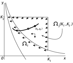
Figure 5: Flow in the set $\Omega_{2}(K_{1},K_{2})$ surrounding an initial point $(x_{0},y_{0})$ outside $\Omega.$

This concludes the proof.  

In the next Proposition we prove results about the rate of convergence of $x(t)$ and $y(t)$ as $t\rightarrow+\infty,$ using an approach akin to Poincaré compactification.

Proposition 2

For any solution $(x,y)$ of (14) we have:

(i)

$\displaystyle{\lim_{t\rightarrow+\infty}\left(\frac{3}{\alpha}t\right)^{1/3}\!\!\!x(t)=1}$

(ii)

$\displaystyle{\lim_{t\rightarrow+\infty}\left(3\alpha^{2}t\right)^{-1/3}y(t)=1}$

(iii)

$\displaystyle{\lim_{t\rightarrow+\infty}\left(\frac{3}{\alpha}t\right)^{2/3}\!\!\!(\alpha-x(t)y(t))=1}$

Proof: For the present proof we found convenient to work with the variable $v:=\alpha-xy$ instead of $y$, and with a new time scale. The idea is essentially that used in Poincaré compactification: to bring to the origin the critical point at infinity, and to turn it into a point of the phase plane by appropriately changing the time scale (cf. eg [34, chap. 5].) By changing variables $(x,y)\mapsto(x,v)$ system (14) becomes

$$\left\{\begin{array}[]{lcl}\dot{x}&=&v-x^{2}\\ \dot{v}&=&\alpha x-2xv-\alpha\frac{v}{x}+\frac{v^{2}}{x}.\end{array}\right.$$ (15)

Suppose $x(0)\neq 0$. Otherwise, since we know by the phase plane analysis in the proof of Proposition 1 that $x(t)>0$ for all $t>0,$ just redefine time so that $x(0)$ becomes positive. Now change the time scale

$$t\mapsto\zeta=\zeta(t):=\int_{0}^{t}\frac{1}{x(s)}ds,$$

and define $\left(\widetilde{x}(\zeta),\widetilde{v}(\zeta)\right):=\left(x(t(\zeta)),v(t(\zeta))\right),$ where $t(\zeta)$ is the inverse function of $\zeta(t)$. By Proposition 1, we have $x(t)\rightarrow 0$ as $t\rightarrow+\infty$, and so also $\zeta\rightarrow+\infty$ as $t\rightarrow+\infty.$ With the new time scale system (15) becomes

$$\left[\begin{array}[]{l}\widetilde{x}\\ \widetilde{v}\end{array}\right]^{\prime}=\left[\begin{array}[]{cr}0&0\\ 0&-\alpha\end{array}\right]\left[\begin{array}[]{c}\widetilde{x}\\ \widetilde{v}\end{array}\right]+\left[\begin{array}[]{c}\widetilde{v}\widetilde{x}-\widetilde{x}^{3}\\ \alpha\widetilde{x}^{2}+\widetilde{v}^{2}-2\widetilde{v}\widetilde{x}^{2}\end{array}\right]$$ (16)

where $(\cdot)^{\prime}=\frac{d}{d\zeta}.$ The region of interest, corresponding to $(x,y)\in\mathbb{R}^{+}\times\mathbb{R}^{+},$ is $(x,v)\in\mathbb{R}^{+}\times(-\infty,\alpha),$ but actually (16) is valid in all of the phase plane $\mathbb{R}^{2}.$ In this way, the critical point at infinity of system (14) is mapped to the critical point at the origin for (16). From the results in Proposition 1 we know that all orbits of (16) obtained from orbits of (14) by the above map will eventually enter $\mathbb{R}^{+}\times(0,\alpha)$ for sufficiently large times $\zeta$ and converge to $(0,0)$ as $\zeta\rightarrow+\infty.$ Using standard results [8, chap. 2] it is straightforward to conclude the existence of a centre manifold for (16) given by

$$\widetilde{v}=\phi(\widetilde{x})\quad{\rm where}\quad\phi(\widetilde{x})=\widetilde{x}^{2}-\frac{1}{\alpha}\widetilde{x}^{4}+{\cal O}(\widetilde{x}^{6}),$$ (17)

that locally attracts all orbits. The dynamics on the centre manifold is given by

$$\widetilde{x}_{c}^{\prime}=-\frac{1}{\alpha}\widetilde{x}_{c}^{5}+{\cal O}(\widetilde{x}_{c}^{7})\quad{\rm as}\;\;\zeta\rightarrow+\infty.$$

Write this differential equation as

$$\frac{d}{d\zeta}\left(\frac{\alpha}{4\widetilde{x}^{4}_{c}}\right)=1+{\cal O}(\widetilde{x}_{c}^{2})\quad{\rm as}\;\;\zeta\rightarrow+\infty.$$ (18)

Fix an initial condition $(\zeta_{0},\widetilde{x}_{0})$ and fix $\varepsilon>0$ arbitrarily. Since we know that $\widetilde{x}_{c}(\zeta)\rightarrow 0$ as $\zeta\to+\infty$ we conclude that there exists a $T>\zeta_{0}$ such that, for all $\zeta>T,$ the following inequalities hold

$$1-\varepsilon\leq\frac{d}{d\zeta}\left(\frac{\alpha}{4\widetilde{x}^{4}_{c}}\right)\leq 1+\varepsilon.$$

Integrating these differential inequalities between $T$ and $\zeta$ we get

$$\frac{\alpha}{4\widetilde{x}^{4}_{T}}+(1-\varepsilon)(\zeta-T)\leq\frac{\alpha}{4\widetilde{x}^{4}}\leq\frac{\alpha}{4\widetilde{x}^{4}_{T}}+(1+\varepsilon)(\zeta-T),$$ (19)

where $\widetilde{x}_{T}=\widetilde{x}(T).$ Dividing (19) by $\zeta$ and taking $\displaystyle{\varliminf_{\zeta\to+\infty}}$ and $\displaystyle{\varlimsup_{\zeta\to+\infty}}$ we obtain

$$1-\varepsilon\leq\varliminf_{\zeta\to+\infty}\frac{\alpha}{4\zeta\widetilde{x}_{c}^{4}}\leq\varlimsup_{\zeta\to+\infty}\frac{\alpha}{4\zeta\widetilde{x}_{c}^{4}}\leq 1+\varepsilon$$

and since $\varepsilon>0$ is arbitrary, we conclude that

$$\lim_{\zeta\to+\infty}\left(\frac{4}{\alpha}\zeta\right)^{1/4}\!\!\widetilde{x}_{c}(\zeta)=1$$ (20)

for solutions corresponding to orbits of (16) on its centre manifold. From standard centre manifold theory [8, chap. 2], long time behaviour of $(\widetilde{x}(\zeta),\widetilde{v}(\zeta))$ is determined by the behaviour on the centre manifold modulo exponentially decaying terms ${\cal O}\left(e^{-\lambda\zeta}\right),$ where $\lambda\in(0,\alpha)$, in particular we can write

$$\widetilde{x}(\zeta)=\widetilde{x}_{c}(\zeta)+{\cal O}\left(e^{-\lambda\zeta}\right).$$

Multiplying this equality by $\left(\frac{4}{\alpha}\zeta\right)^{1/4}$ and using (20) we conclude that

$$\lim_{\zeta\to+\infty}\left(\frac{4}{\alpha}\zeta\right)^{1/4}\!\!\widetilde{x}(\zeta)=1.$$ (21)

We can do the same for the evolution of the $\widetilde{v}$ variable: for orbits on the centre manifold we have $\widetilde{v}_{c}=\widetilde{x}_{c}^{2}+{\cal O}(\widetilde{x}_{c}^{4}),$ multiplying this by $\left(\frac{4}{\alpha}\zeta\right)^{1/2},$ and using (20) we conclude that

$$\lim_{\zeta\to+\infty}\left(\frac{4}{\alpha}\zeta\right)^{1/2}\!\!\widetilde{v}_{c}(\zeta)=1.$$

To obtain the dynamics outside the centre manifold we proceed as with the $\widetilde{x}$ variable and get

$$\lim_{\zeta\to+\infty}\left(\frac{4}{\alpha}\zeta\right)^{1/2}\!\!\widetilde{v}(\zeta)=1.$$ (22)

In order to obtain the corresponding rate estimates in the original time variable $t$ we need to relate the asymptotics of both time scales. By the definition of the new time scale

$$\zeta(t)-\zeta(t_{0})=\int_{t_{0}}^{t}\!\frac{1}{x(s)}ds$$

and so $\frac{d\zeta}{dt}=\frac{1}{x(t)}.$ Hence, by the inverse function theorem, $\frac{dt}{d\zeta}=\widetilde{x}(\zeta),$ and thus

$$t(\zeta)-t(\zeta_{0})=\int_{\zeta_{0}}^{\zeta}\widetilde{x}(s)ds$$ (23)

where $\zeta_{0}=\zeta(t_{0}).$ From (21) we know that

$$\forall\varepsilon>0,\,\exists T=T(\varepsilon):\,\forall\zeta>T,\,\left(\frac{4}{\alpha}\zeta\right)^{1/4}\!\!\widetilde{x}(\zeta)\in[1-\varepsilon,1+\varepsilon]$$ (24)

Let us look first at the upper bound: for all $\zeta>T,$

$$\widetilde{x}(\zeta)\leq\left(\frac{4}{\alpha}\zeta\right)^{-1/4}(1+\varepsilon),$$

substituting this into (23) we get, for $\zeta_{0}\geq T,$

$$t(\zeta)-t(\zeta_{0}) \leq \int_{\zeta_{0}}^{\zeta}\left(\frac{4}{\alpha}s\right)^{-1/4}\!\!(1+\varepsilon)ds$$

$$= (1+\varepsilon)\left(\frac{\alpha}{4}\right)^{1/4}\frac{4}{3}\left(\zeta^{3/4}-\zeta_{0}^{3/4}\right).$$

Multiplying this inequality by $\frac{3}{4}\left(\frac{4}{\alpha}\right)^{1/4}\zeta^{-3/4}$ and passing to the limit as $\zeta\to+\infty$ results in

$$\varlimsup_{\zeta\to+\infty}\frac{3}{4}\left(\frac{4}{\alpha}\right)^{1/4}\!\!\zeta^{-3/4}t(\zeta)\leq 1+\varepsilon.$$

Using the lower bound of (24) and the same argument we obtain the reverse bound

$$\varliminf_{\zeta\to+\infty}\frac{3}{4}\left(\frac{4}{\alpha}\right)^{1/4}\!\!\zeta^{-3/4}t(\zeta)\geq 1-\varepsilon.$$

and by the arbitrariness of $\varepsilon>0$ we get

$$\frac{3}{4}\left(\frac{4}{\alpha}\right)^{1/4}\!\!\zeta^{-3/4}t(\zeta)=1+{\scriptstyle\cal O}(1)\quad\text{as $\zeta\to+\infty$},$$ (25)

which, together with (21) and (22), allow us to conclude that, as $t\rightarrow+\infty$ (ie, as $\zeta\to+\infty$)

$$\left(\frac{3}{\alpha}t\right)^{1/3}\!\!\!x(t)=\left(\frac{4}{\alpha}\zeta\right)^{1/4}\!\!\!\widetilde{x}(\zeta)(1+{\scriptstyle\cal O}(1))=1+{\scriptstyle\cal O}(1),$$

and

$$\left(\frac{3}{\alpha}t\right)^{2/3}\!\!\!v(t)=\left(\frac{4}{\alpha}\zeta\right)^{1/2}\!\!\!\widetilde{v}(\zeta)(1+{\scriptstyle\cal O}(1))=1+{\scriptstyle\cal O}(1),$$

thus proving (i) and (iii) respectively.

Finally, to prove (ii), observe that for the original variable $y(t)$ we have $y=\frac{\alpha-v}{x}$ and thus, as $t\rightarrow+\infty$,

$$(3\alpha^{2}t)^{-1/3}y(t)=\frac{1}{\left(\frac{3}{\alpha}t\right)^{1/3}\!\!x(t)}-\frac{\left(\frac{3}{\alpha}t\right)^{2/3}\!\!v(t)}{\left(\frac{3}{\alpha}t\right)^{1/3}\!\!x(t)}\,\frac{1}{\alpha\left(\frac{3}{\alpha}t\right)^{2/3}}\rightarrow 1$$

which concludes the proof.  

4 Long time behaviour of the system

We now turn our attention to the long-time behaviour of $c_{j}(t)$ with $j\geq 2$. It is convenient to consider the time scale introduced in Section 2. The first result we need is the following, the proof of which is entirely analogous to that of the corresponding results presented in the second half of the proof of Proposition 2, and so we refrain from repeating it here,

Proposition 3

With $(c_{j})$, $\tau$, and $(\widetilde{c}_{j})$ as given in (6) and (7), the following holds true:

(i)

$\displaystyle{\lim_{t\rightarrow+\infty}\frac{2}{3}\left(\frac{3}{\alpha}\right)^{1/3}\!\!\!t^{-2/3}\tau(t)=1}$;

(ii)

$\displaystyle{\lim_{\tau\rightarrow+\infty}\sqrt{\frac{2\tau}{\alpha}\,}\;\widetilde{c}_{1}(\tau)=1}$;

With this knowledge, we can now use (8) to get information on the long time behaviour of $\widetilde{c}_{j}(\tau)$ for $j\geq 2,$ specifically, we prove now that (ii) in Proposition 3 holds for all $\widetilde{c}_{j}(\tau)$. To see this, multiply (8) by $\sqrt{\frac{2\tau}{\alpha}}.$ The first term in the right hand side of the resulting expression is the contribution due to the non monomeric initial data, and since $j$ is fixed, we have, as $\tau\rightarrow+\infty$,

$$\tau^{\frac{1}{2}}e^{-\tau}\sum_{k=2}^{j}\frac{\tau^{j-k}}{(j-k)!}c_{k}(0)={\cal O}\left(\tau^{j-\frac{3}{2}}e^{-\tau}\right)={\scriptstyle\cal O}\left(e^{-\lambda\tau}\right),$$

for every $\lambda<1.$ In order to study the remaining integral term, first change the integration variable $s\mapsto y=s/\tau$ in order to get the integral in a fixed bounded region, and define the function $\psi(\cdot):=\sqrt{\frac{2}{\alpha}\,(\cdot)\,}\,\widetilde{c}_{1}(\cdot).$ We thus get

$$\sqrt{\frac{2\tau}{\alpha}}\frac{1}{(j-2)!}\int_{0}^{\tau}\widetilde{c}_{1}(\tau-s)s^{j-2}e^{-s}ds=\frac{\tau^{j-1}}{(j-2)!}\int_{0}^{1}\frac{\psi(\tau(1-y))y^{j-2}}{\sqrt{1-y}}e^{-\tau y}dy.$$

Let $0<\varepsilon<1$ be fixed, and write the integral as $\int_{0}^{1-\varepsilon}+\int_{1-\varepsilon}^{1}.$ The last integral is fairly easy to handle: Since $\psi(s)$ is a continuous function and, by Proposition 3, is $1+{\scriptstyle\cal O}(1)$ as $s\rightarrow+\infty,$ we conclude that it is bounded in $[0,\infty)$ and so there exists a positive constant $M_{\psi}$ such that $0\leq\psi(s)\leq M_{\psi}$ for all $s.$ From this it follows that

$$\tau^{j-1}\int_{1-\varepsilon}^{1}\frac{\psi(\tau(1-y))y^{j-2}}{\sqrt{1-y}}e^{-\tau y}dy \leq M_{\psi}\tau^{j-1}e^{-(1-\varepsilon)\tau}\int_{1-\varepsilon}^{1}\frac{y^{j-2}}{\sqrt{1-y}}dy$$

$$< M_{\psi}\tau^{j-1}e^{-(1-\varepsilon)\tau}\int_{1-\varepsilon}^{1}\frac{1}{\sqrt{1-y}}dy$$

$$< 2\sqrt{\varepsilon}M_{\psi}\tau^{j-1}e^{-(1-\varepsilon)\tau},$$

and so it is also exponentially small when $\tau\rightarrow+\infty.$ For the integral over $(0,1-\varepsilon)$ we use $y<1-\varepsilon\Rightarrow\tau(1-y)>\tau\varepsilon\rightarrow+\infty$ as $\tau\rightarrow+\infty,$ and Proposition 3 (ii) to conclude that $\psi=1+{\scriptstyle\cal O}(1)$ in the region of integration, provided $\tau$ is sufficiently large. Therefore, $\forall\delta>0,\,\exists T(\delta):\,\forall\tau>T(\delta),\,\psi(\tau(1-y))\in[1-\delta,1+\delta]$, and, as $\tau\rightarrow+\infty,$

$$(1-\delta)I_{0,j}(\tau)\leq\int_{0}^{1-\varepsilon}\frac{\psi(\tau(1-y))y^{j-2}}{\sqrt{1-y}}e^{-\tau y}dy\leq(1+\delta)I_{0,j}(\tau)$$ (26)

with

$$I_{0,j}(\tau):=\int_{0}^{1-\varepsilon}\frac{y^{j-2}}{\sqrt{1-y}}e^{-\tau y}dy.$$

This integral is easily estimated using Watson’s Lemma [2, pp 427-8]: from the Taylor expansion

$$\frac{y^{j-2}}{\sqrt{1-y}}=y^{j-2}\sum_{k=0}^{\infty}\frac{(2k-1)!!}{(2k)!!}y^{k},$$

which converges for $|y|<1,$ we can apply Watson’s Lemma directly to get

$$I_{0,j}(\tau)=\frac{\Gamma(j-1)}{\tau^{j-1}}+{\cal O}\left(\tau^{-j}\right),\quad\mbox{\rm as}\;\tau\rightarrow+\infty.$$

Plugging this into (26) immediately results in

$$\frac{\tau^{j-1}}{(j-2)!}\int_{0}^{1-\varepsilon}\frac{\psi(\tau(1-y))y^{j-2}}{\sqrt{1-y}}e^{-\tau y}dy=1+{\cal O}\left(\tau^{-1}\right)\quad\mbox{\rm as}\;\tau\rightarrow+\infty.$$

This, together with the other two exponentially small contributions proved above, implies that $\sqrt{\frac{2\tau}{\alpha}\,}\;\widetilde{c}_{j}(\tau)\longrightarrow 1,$ as $\tau\rightarrow+\infty,$ for all $j\geq 2,$ thus complementing part (ii) of Proposition 3. Using part (i) we can easily translate this behaviour to the original time scale, and conclude the following:

Theorem 2

Let $(c_{j})$ be any non-negative solution of (3) with initial data satisfying $c_{0}(0)=\sum_{j=1}^{\infty}c_{j}(0)<\infty$. Then, as $t\rightarrow+\infty$, we have

(i)

$\displaystyle{\left(\frac{3}{\alpha}t\right)^{1/3}\!\!\!c_{j}(t)\longrightarrow 1}$     for all $j\geq 1$;

(ii)

$\displaystyle{\left(3\alpha^{2}t\right)^{-1/3}\sum_{j=1}^{\infty}c_{j}(t)\longrightarrow 1}$;

(iii)

$\displaystyle{\left(\frac{3}{\alpha}t\right)^{2/3}\!\!\left(\alpha-c_{1}(t)\sum_{j=1}^{\infty}c_{j}(t)\right)\longrightarrow 1}$.

5 Self-similar behaviour of the coagulation system outside the characteristic direction

We have now reached the main objective of the paper: the study of convergence to similarity profiles in this addition model.

Let $\Phi_{1}:\mathbb{R}^{+}\setminus\{1\}\rightarrow\mathbb{R}$ be the function given by

$$\Phi_{1}(\eta):=\begin{cases}\displaystyle{\frac{1}{\sqrt{1-\eta}}}&\text{if $\eta<1$},\\ 0&\text{if $\eta>1$}.\end{cases}$$

The main result in this part is the following:

Theorem 3

Let $(c_{j})$ be any non-negative solution of (3) with initial data satisfying $\exists\rho>0,\mu>\frac{1}{2}:\forall j,c_{j}(0)\leq\rho/j^{\mu}$. Let $\tau(t)$ and $\widetilde{c}_{j}(\tau)$ be as given in (6) and (7) respectively. Then,

$$\lim_{\begin{subarray}{c}j,\,\tau\rightarrow+\infty\\ \eta=j/\tau\;{\rm fixed}\\ \eta\neq 1\end{subarray}}\sqrt{\frac{2}{\alpha}\tau\,}\;\widetilde{c}_{j}(\tau)=\Phi_{1}(\eta)$$

Proof
Expression (8) describes the time evolution of $\widetilde{c}_{j}(\tau)$ by the sum of a contribution dependent only on the non-monomeric part of the initial data with a term determined by the behaviour of $c_{1}(t)$ in the appropriate time scale. For monomeric initial data, only this last term is relevant, and we start our analysis by it.

5.1 Monomeric initial data

Assuming monomeric initial conditions we have, for $j\geq 2,$

$$\sqrt{\frac{2}{\alpha}\tau\,}\;\widetilde{c}_{j}(\tau)=\frac{\sqrt{\frac{2}{\alpha}\tau\,}}{(j-2)!}\int_{0}^{\tau}\widetilde{c}_{1}(\tau-s)s^{j-2}e^{-s}ds.$$ (27)

Consider the function $\varphi_{1}$ defined in $[2,\infty)\times[0,\infty)$ by

$$\varphi_{1}(x,\tau):=\frac{\sqrt{\frac{2}{\alpha}\tau\,}}{\Gamma(x-1)}\int_{0}^{\tau}\widetilde{c}_{1}(\tau-s)s^{x-2}e^{-s}ds.$$ (28)

Clearly $\varphi_{1}=\sqrt{\frac{2}{\alpha}\tau}\,\widetilde{c}\;$ if $2\leq x=j\in\mathbb{N}$, and the use of $\varphi_{1}$ is a good deal more convenient in order to obtain the required asymptotic results. So we now concentrate on (28). Let $\eta:=x/\tau.$ By changing variable $s\mapsto y=s/\tau,$ using the recursive relation $\Gamma(x-1)=\Gamma(x)/(x-1),$ and Stirling’s asymptotic formula $\Gamma(x)=e^{-x}x^{x-\frac{1}{2}}\sqrt{2\pi}\left(1+{\cal O}(x^{-1})\right)$ as $x\rightarrow\infty$, we can write, as $\tau\rightarrow+\infty,$

$$\varphi_{1}(\eta\tau,\tau)=\frac{\eta^{\frac{3}{2}-\eta\tau}\tau^{\frac{1}{2}}}{\sqrt{\alpha\pi}}\left(1+{\cal O}\left(\tau^{-1}\right)\right)\int_{0}^{1}\frac{\widetilde{c}_{1}(\tau(1-y))\tau^{1/2}e^{\tau(\eta\log y-y+\eta)}}{y^{2}}dy.$$ (29)

In order to make use of our knowledge about the long time behaviour of $\widetilde{c}_{1}(\tau)$ given in Proposition 3 it is convenient to rearrange the integrand of (29) by multiplying and dividing it by $\sqrt{\frac{2}{\alpha}(1-y)}$, resulting in the following, as $\tau\rightarrow+\infty,$

$$\varphi_{1}(\eta\tau,\tau)=\frac{1}{\sqrt{2\pi}}\eta^{\frac{3}{2}-\eta\tau}\tau^{\frac{1}{2}}\left(1+{\cal O}\left(\tau^{-1}\right)\right)\int_{0}^{1}\psi(\tau(1-y))\frac{e^{\tau(\eta\log y-y+\eta)}}{y^{2}\sqrt{1-y}}dy,$$ (30)

where $\psi(\cdot):=\sqrt{\frac{2}{\alpha}\,(\cdot)\,}\,\widetilde{c}_{1}(\cdot)$ is the function that was already defined and used in Section 4. The proof now reduces to the asymptotic evaluation of the function

$$I(\eta,\tau):=\tau^{\frac{1}{2}}\eta^{-\eta\tau}e^{\tau\eta}\int_{0}^{1}\psi(\tau(1-y))\frac{e^{\tau(\eta\log y-y)}}{y^{2}\sqrt{1-y}}dy$$ (31)

as $\tau\rightarrow+\infty.$

We first consider the case $\eta>1.$

Observe that $y^{-2}e^{\tau(\eta\log y-y)}=e^{(\eta\tau-2)\log y-\tau y}=:e^{g_{1}(y)},$ where $g_{1}:\mathbb{R}^{+}\rightarrow\mathbb{R}$, defined by the last equality, satisfies, for all $y\in(0,1]$ and $\tau>\frac{2}{\eta-1}$

$$g_{1}^{\prime}(y)=\frac{\eta\tau-2}{y}-\tau\geq(\tau\eta-2)-\tau>0.$$

Therefore, $g_{1}(y)\leq g_{1}(1)=-\tau,$ and so

$$\int_{0}^{1}\psi(\tau(1-y))\frac{e^{\tau(\eta\log y-y)}}{y^{2}\sqrt{1-y}}dy\leq M_{\psi}e^{-\tau}\int_{0}^{1}\frac{1}{\sqrt{1-y}}dy=2M_{\psi}e^{-\tau}.$$

Plugging into (31) we obtain, as $\tau\rightarrow+\infty,$ $I(\eta,\tau)\leq C\tau^{\frac{1}{2}}e^{-\tau(\eta\log\eta-\eta+1)}$ for some positive constant $C.$ Since $\eta\log\eta-\eta+1>0$ for all $\eta>1$, we conclude that $I(\eta,\tau)\rightarrow 0$ as $\tau\rightarrow+\infty,$ and this proves the result when $\eta>1.$

Consider now the case $\eta\in(0,1)$.

Observe first that the exponential term inside the integral in (31) has a unique maximum at $y=\eta$. Therefore, in order to estimate (31) when $\tau\rightarrow+\infty$ we are going to study its behaviour around the maximum separately from the other cases. To this end, let $\varepsilon<\min\{\eta e^{-1},1-\eta\}$ and write

$$I(\eta,\tau) = \tau^{\frac{1}{2}}\eta^{-\eta\tau}e^{\tau\eta}\left(\int_{0}^{\varepsilon}+\int_{\varepsilon}^{1-\varepsilon}+\int_{1-\varepsilon}^{1}\right)\psi(\tau(1-y))\frac{e^{\tau(\eta\log y-y)}}{y^{2}\sqrt{1-y}}dy$$ (32)

$$=: I_{1}(\eta,\tau)+I_{2}(\eta,\tau)+I_{3}(\eta,\tau).$$

The study of the integral $I_{1}(\eta,\tau)$ is entirely analogous to what was done in the case $\eta>1:$ since $0<y<\varepsilon<\eta e^{-1}<\eta$ we now have, for all $\tau>\frac{2}{(1-e^{-1})\eta}$,

$$g_{1}^{\prime}(y)=\frac{\eta\tau-2}{y}-\tau=\frac{\tau(\eta-y)-2}{y}>0.$$

Thus, $g_{1}(y)\leq g_{1}(\varepsilon)<g_{1}(\eta e^{-1})=(\eta\tau-2)\log\eta-(\eta\tau-2)-\tau\eta e^{-1},$ and we can write

$$I_{1}(\eta,\tau) \leq \tau^{\frac{1}{2}}e^{\tau\eta(1-\log\eta)+(\eta\tau-2)\log\eta-(\eta\tau-2)-\tau\eta/e}M_{\psi}\int_{0}^{\varepsilon}\frac{1}{\sqrt{1-y}}dy$$ (33)

$$\leq C\tau^{\frac{1}{2}}e^{-\tau\eta/e}\longrightarrow 0\quad{\rm as}\;\tau\rightarrow+\infty,$$

for some positive constant $C.$

For the integral $I_{3}(\eta,\tau)$, define the function $g_{3}:(0,1)\rightarrow\mathbb{R}$ by $g_{3}(y):=(\eta\log\eta-\eta)-(\eta\log y-y).$ Since $g_{3}$ has a unique minimum at $y=\eta$, where its value is $g_{3}(\eta)=0,$ we conclude that $y>1-\varepsilon>\eta\Rightarrow g_{3}(y)>g_{3}(1-\varepsilon)>0$ and thus, there exists a positive constant $C$ such that

$$I_{3}(\eta,\tau) = \tau^{\frac{1}{2}}\int_{1-\varepsilon}^{1}\psi(\tau(1-y))\frac{e^{-\tau g_{3}(y)}}{y^{2}\sqrt{1-y}}dy$$ (34)

$$\leq C\tau^{\frac{1}{2}}e^{-\tau g_{3}(1-\varepsilon)}\longrightarrow 0\quad{\rm as}\;\tau\rightarrow+\infty,$$

From (33) and (34) we conclude that

$$I(\eta,\tau)=I_{2}(\eta,\tau)+{\scriptstyle\cal O}(1)\quad{\rm as}\;\tau\rightarrow+\infty.$$ (35)

In order to estimate $I_{2}(\eta,\tau)$ we proceed as follows: we now have $\tau(1-y)>\tau\varepsilon\rightarrow+\infty$ as $\tau\rightarrow+\infty,$ and thus $\psi(\tau(1-y))=1+{\scriptstyle\cal O}(1)$ when evaluating $I_{2}$ for large values of $\tau.$ As in a similar situation in Section 4, we have $\forall\delta>0,\,\exists T(\delta):\,\forall\tau>T(\delta),\,\psi(\tau(1-y))\in[1-\delta,1+\delta]$, and we can estimate

$$(1-\delta)\tau^{\frac{1}{2}}\eta^{-\eta\tau}J(\eta,\tau)\leq I_{2}(\eta,\tau)\leq(1+\delta)\tau^{\frac{1}{2}}\eta^{-\eta\tau}J(\eta,\tau)\quad\text{as $\tau\rightarrow+\infty,$}$$ (36)

with

$$J(\eta,\tau):=\int_{\varepsilon}^{1-\varepsilon}\frac{1}{y^{2}\sqrt{1-y}}e^{-\tau\phi(y)}dy,$$

and $\phi:(0,1)\rightarrow\mathbb{R}$ is defined by $\phi(y):=y-\eta\log y-\eta.$ Since this function is smooth and has a unique minimum, attained at $y=\eta\in(\varepsilon,1-\varepsilon)$ with value $\phi(\eta)=-\eta\log\eta$ and $\phi^{\prime\prime}(\eta)=\eta^{-1},$ Laplace’s method for the asymptotic evaluation of integrals [2, pg 431] is applicable to $J(\eta,\tau)$, and we obtain, as $\tau\rightarrow+\infty,$

$$J(\eta,\tau)=e^{\tau\eta\log\eta}\frac{1}{\eta^{2}\sqrt{1-\eta}}\sqrt{\frac{2\pi}{\tau/\eta}}+{\cal O}\left(\frac{e^{\tau\eta\log\eta}}{\tau^{3/2}}\right).$$ (37)

Hence, from (30), (31), (35), (36) and (37), we can write, as $\tau\rightarrow+\infty,$

$$\varphi_{1}(\eta\tau,\tau) = \;\;\frac{1}{\sqrt{2\pi}}\eta^{\frac{3}{2}-\eta\tau}\tau^{\frac{1}{2}}e^{\tau\eta\log\eta}\frac{1}{\eta^{2}\sqrt{1-\eta}}\sqrt{\frac{2\pi}{\tau/\eta}}\left(1+{\cal O}\left(\tau^{-1}\right)\right)$$ (39)

$$\!+\,\frac{1}{\sqrt{2\pi}}\eta^{\frac{3}{2}-\eta\tau}\tau^{\frac{1}{2}}{\cal O}\left(\frac{e^{\tau\eta\log\eta}}{\tau^{3/2}}\right)\left(1+{\cal O}\left(\tau^{-1}\right)\right)+{\scriptstyle\cal O}(1)$$

After a few trivial calculations, we imediately recognize that, as $\tau\rightarrow+\infty,$ (39) is equal to $\frac{1}{\sqrt{1-\eta}}(1+{\scriptstyle\cal O}(1)),$ and (39) is $\tau^{-1}{\cal O}(1)\left(1+{\cal O}\left(\tau^{-1}\right)\right)+{\scriptstyle\cal O}(1)={\cal O}\left(\tau^{-1}\right)+{\scriptstyle\cal O}(1)={\scriptstyle\cal O}(1).$ Therefore, for $\eta\in(0,1),$

$$\varphi_{1}(\eta\tau,\tau)\longrightarrow\frac{1}{\sqrt{1-\eta}}\quad\text{as $\tau\rightarrow+\infty$}$$

and this concludes the proof in the case of monomeric initial data.

5.2 Non monomeric initial data

If the initial data has non zero components $c_{k}(0)$ with $k\geq 2,$ the proof of the stated similarity behaviour of $\widetilde{c}_{j}(\tau)$ requires, according to (8), that we now prove that

$$\lim_{\begin{subarray}{c}j,\,\tau\rightarrow+\infty\\ \eta=j/\tau\;{\rm fixed}\\ \eta\neq 1\end{subarray}}\sqrt{\frac{2}{\alpha}\tau\,}\;e^{-\tau}\sum_{k=2}^{j}\frac{\tau^{j-k}}{(j-k)!}c_{k}(0)=0.$$

Define $\nu:=\eta^{-1}$, write $\tau=j\nu,$ and use the assumption on the initial condition, namely $c_{k}(0)\leq\rho/k^{\mu}.$ We thus have

$$\sqrt{\frac{2}{\alpha}\tau\,}\;e^{-\tau}\sum_{k=2}^{j}\frac{\tau^{j-k}}{(j-k)!}c_{k}(0) \leq \rho\sqrt{\frac{2}{\alpha}\,}\sqrt{j\nu}\;e^{-j\nu}\sum_{k=2}^{j}\frac{(j\nu)^{j-k}}{(j-k)!k^{\mu}}$$

$$=: \rho\sqrt{\frac{2}{\alpha}\,}\varphi_{2}(\nu,j)$$

where $\varphi_{2}$ is defined by the equality. Our goal is to prove that $\varphi_{2}(\nu,j)\rightarrow 0$ as $j\rightarrow\infty$, for all positive $\nu\neq 1.$

Like it was done before, we shall study the cases $\nu>1$ and $\nu<1$ separately. By the heuristic geometric reasons explained in the Introduction, the case $\nu>1$ ($\eta<1$) is now easier to handle. In fact, for this case, even using the notoriously bad upper bound to the sum provided by taking the product of the number of terms by their maximum, we only need to impose $\mu\geq 0$. Using this same approach to estimate $\varphi_{2}$ in the case $\nu<1$ ($\eta>1$) we would need to impose $\mu>1,$ which would not even guarantee that all finite mass initial data are included. So, for this second part of the proof, a finer approach is required, which consists in estimating the small and the large $\ell$ contributions to $\varphi_{2}$ separately.

Consider first the case $\nu>1.$

Change the summation variable $k\mapsto\ell:=j-k.$ It is sufficient, for this range of $\nu$, to bound $\varphi_{2}$ as follows

$$\varphi_{2}(\nu,j)=\sqrt{j\nu}\;e^{-j\nu}\sum_{\ell=0}^{j-2}\frac{(j\nu)^{\ell}}{\ell!(j-\ell)^{\mu}}\leq\frac{1}{2^{\mu}}\sqrt{j\nu}\;e^{-j\nu}\sum_{\ell=0}^{j-2}\frac{(j\nu)^{\ell}}{\ell!}.$$ (40)

Considering the sequence $u_{\ell}:=\frac{(j\nu)^{\ell}}{\ell!},$ and studying the sign of

$$u_{\ell+1}-u_{\ell}=\frac{(j\nu)^{\ell}}{\ell!}\left(\frac{j\nu}{\ell+1}-1\right),$$

we conclude the maximum of $u_{\ell}$ is attained at $\ell=\lfloor j\nu\rfloor>j\nu-1>j-1>j-2.$ As $j\rightarrow\infty$, we can thus estimate the right-hand side of (40):

$$\frac{1}{2^{\mu}}\sqrt{j\nu}\;e^{-j\nu}\sum_{\ell=0}^{j-2}\frac{(j\nu)^{\ell}}{\ell!} < \frac{1}{2^{\mu}}\sqrt{j\nu}\;e^{-j\nu}(j-1)\frac{(j\nu)^{j-2}}{(j-2)!}$$

$$= \frac{1}{2^{\mu}}(j\nu)^{-3/2}\;e^{-j\nu}(j-1)^{2}\frac{(j\nu)^{j}}{(j-1)!}$$

$$= \frac{\nu^{-3/2}}{2^{\mu}\sqrt{2\pi}}j^{-3/2}\;e^{-j\nu}(j-1)^{2}\frac{(j\nu)^{j}}{e^{-j}j^{j}j^{-1/2}}(1+{\scriptstyle\cal O}(1))$$

$$= \frac{\nu^{-3/2}}{2^{\mu}\sqrt{2\pi}}\left(\frac{j-1}{j}\right)^{2}e^{-j(\nu-1-\log\nu)+\log j}(1+{\scriptstyle\cal O}(1))$$

where we use Stirling’s approximation in the second equality. Since $\nu>1,$ we have $\nu-1-\log\nu>0$, and so $-j(\nu-1-\log\nu)+\log j\rightarrow-\infty$ as $j\rightarrow\infty$ from which we conclude (LABEL:**) goes to zero as $j\rightarrow\infty,$ and we obtain the result we seek in the case $\nu>1.$

Consider now the case $\nu\in(0,1).$

Let $\beta\in\left(\nu e^{1-\nu},\min\{\nu e,1\}\right)$ be fixed, and write

$$\varphi_{2}(\nu,j)=\sqrt{j\nu}\;e^{-j\nu}\left(\sum_{0\leq\ell\leq\beta j}\frac{(j\nu)^{\ell}}{\ell!(j-\ell)^{\mu}}+\sum_{\beta j<\ell\leq j-2}\frac{(j\nu)^{\ell}}{\ell!(j-\ell)^{\mu}}\right)=:S_{1}(j)+S_{2}(j)$$

For the first sum we have

$$S_{1}(j) \leq \sqrt{j\nu}\;e^{-j\nu}\sum_{0\leq\ell\leq\beta j}\frac{(j\nu)^{\ell}}{\ell!(j-\beta j)^{\mu}}$$

$$= \sqrt{j\nu}\;e^{-j\nu}\frac{1}{j^{\mu}(1-\beta)^{\mu}}\sum_{0\leq\ell\leq\beta j}\frac{(j\nu)^{\ell}}{\ell!}$$

$$\leq \sqrt{j\nu}\;e^{-j\nu}\frac{1}{j^{\mu}(1-\beta)^{\mu}}e^{j\nu}$$

$$= \frac{\sqrt{\nu}}{(1-\beta)^{\mu}}j^{\frac{1}{2}-\mu}\longrightarrow 0\quad\mbox{as}\;\,j\rightarrow\infty,\;\,\mbox{if}\;\,\mu>\frac{1}{2}.$$

By Stirling’s expansion we can write, for all sufficiently large $\ell,$ $\ell!\geq e^{-\ell}\ell^{\ell+\frac{1}{2}}.$ Therefore, since in $S_{2}$ we have $(j-\ell)^{\mu}\geq 2^{\mu}\geq 1,$ we can estimate that term as follows,

$$S_{2}(j) \leq \sqrt{j\nu}\;e^{-j\nu}\sum_{\beta j<\ell\leq j-2}\frac{(j\nu)^{\ell}}{e^{-\ell}\ell^{\ell+\frac{1}{2}}}$$

$$= \sqrt{j\nu}\;e^{-j\nu}\sum_{\beta j<\ell\leq j-2}\ell^{-\frac{1}{2}}\left(\frac{j\nu e}{\ell}\right)^{\ell}$$

$$< \sqrt{\frac{\nu}{\beta}}\;e^{-j\nu}\sum_{\beta j<\ell\leq j-2}\left(\frac{j\nu e}{\ell}\right)^{\ell}$$

$$< \sqrt{\frac{\nu}{\beta}}\;e^{-j\nu}\frac{1-\left(\frac{\nu e}{\beta}\right)^{j-2-\lfloor\beta j\rfloor}}{1-\frac{\nu e}{\beta}}\left(\frac{\nu e}{\beta}\right)^{\lfloor\beta j\rfloor+1}$$

$$< \frac{\sqrt{\nu\beta}}{\nu e-\beta}\;e^{-j\nu}\left(\frac{\nu e}{\beta}\right)^{j-1}$$

$$= \frac{\sqrt{\nu\beta}}{\nu e-\beta}\frac{\beta}{\nu e}\left(\frac{\nu e^{1-\nu}}{\beta}\right)^{j}\longrightarrow 0\quad\mbox{as}\;\,j\rightarrow\infty.$$

This completes the proof of the theorem.  

6 Self-similar behaviour of the coagulation system along the characteristic direction

Consider the function $\Phi_{2}:\mathbb{R}\rightarrow\mathbb{R}$ defined by

$$\Phi_{2}(\xi):=e^{-\frac{1}{2}\xi^{2}}\!\int_{0}^{+\infty}\!\!e^{-\xi w^{2}-\frac{1}{2}w^{4}}dw.$$

The main result of this part of the paper, complementing Theorem 3, is the following

6.1 Monomeric initial data

Theorem 4

Let $(c_{j})$ be any non-negative solution of (3) with monomeric initial data. Let $\tau(t)$ and $\widetilde{c}_{j}(\tau)$ be as given in (6) and (7) respectively. Then,

$$\lim_{\begin{subarray}{c}j,\,\tau\rightarrow+\infty\\ \xi=\frac{j-\tau}{\sqrt{\tau}}\;{\rm fixed}\\ \xi\in\mathbb{R}\end{subarray}}\left(\frac{\pi^{2}}{\alpha^{2}}\tau\!\right)^{1/4}\!\widetilde{c}_{j}(\tau)=\Phi_{2}(\xi).$$

After a few manipulations with the integral defining $\Phi_{2}$ we can write

$$\Phi_{2}(\xi)=\frac{\pi}{4}\sqrt{|\xi|}e^{-\frac{1}{4}\xi^{2}}\left(I_{-\frac{1}{4}}\left(\tfrac{1}{4}\xi^{2}\right)+\operatorname{{sgn}}(-\xi)I_{\frac{1}{4}}\left(\tfrac{1}{4}\xi^{2}\right)\right),$$

where $I_{\nu}(\cdot)$ is the modified Bessel function [1, pp 374-7], and the value at $\xi=0$ is defined to be the limit of the right-hand side as $\xi\rightarrow 0.$ Actually, $\Phi_{2}$ can be seen as an element of a larger family of functions: it is the function obtained by making $\nu=\frac{1}{2}$ in

$$\begin{array}[]{l}g_{\nu}(\xi):=\\ :=\frac{\Gamma(1-\tfrac{1}{2}\nu)|\xi|e^{-\frac{1}{2}\xi^{2}}}{2^{\nu/2-1/2}\sqrt{\pi}}\left(\frac{\Gamma\left(\tfrac{1}{2}-\tfrac{1}{2}\nu\right)}{4\sqrt{\pi}}U\left(1-\tfrac{1}{2}\nu,\tfrac{3}{2};\tfrac{1}{2}\xi^{2}\right)+\tfrac{\operatorname{{sgn}}(-\xi)+1}{2}M\left(1-\tfrac{1}{2}\nu,\tfrac{3}{2};\tfrac{1}{2}\xi^{2}\right)\right).\end{array}$$

These functions were formally deduced in [31] as similarity profiles for addition models with time dependent monomer inputs $J_{0}(t)=\alpha t^{\omega},$ where $\nu=-\frac{\omega-1}{\omega+2}.$ The functions $U$ and $M$ are Kummer’s hypergeometric functions [1, pp 504-515].

Proof

For monomeric initial data (8) reduces to

$$\left(\frac{\pi^{2}}{\alpha^{2}}\tau\!\right)^{1/4}\!\widetilde{c}_{j}(\tau)=\frac{\left(\frac{\pi^{2}}{\alpha^{2}}\tau\!\right)^{1/4}}{(j-2)!}\int_{0}^{\tau}\widetilde{c}_{1}(\tau-s)s^{j-2}e^{-s}ds.$$

Consider the function $\varphi_{3}$ defined in $[2,\infty)\times[0,\infty)$ by

$$\varphi_{3}(x,\tau):=\frac{\left(\frac{\pi^{2}}{\alpha^{2}}\tau\!\right)^{1/4}}{\Gamma(x-1)}\int_{0}^{\tau}\widetilde{c}_{1}(\tau-s)s^{x-2}e^{-s}ds.$$ (42)

In order to consider the similarity limit we introduce the variable $\xi:=\frac{j-\tau}{\sqrt{\tau}}$ and write (42) in the similarity variable $\xi$ as follows:

$$\varphi_{3}(\tau+\xi\sqrt{\tau},\tau):=\frac{\left(\frac{\pi^{2}}{\alpha^{2}}\tau\!\right)^{1/4}}{\Gamma(\tau+\xi\sqrt{\tau}-1)}\int_{0}^{\tau}\widetilde{c}_{1}(\tau-s)s^{\tau+\xi\sqrt{\tau}-2}e^{-s}ds.$$ (43)

Since $\varphi_{3}(j,\tau)=\left(\frac{\pi^{2}}{\alpha^{2}}\tau\!\right)^{1/4}\!\widetilde{c}_{j}(\tau)$ if $2\leq x=j\in\mathbb{N}$, to prove the theorem it suffices to show that

$$\lim_{\tau\rightarrow+\infty}\varphi_{3}(\tau+\xi\sqrt{\tau},\tau)=\Phi_{2}(\xi).$$ (44)

We start by considering, in the integral in the right-hand side of (43), the change of variables

$$s\mapsto w:=\sqrt{\sqrt{\tau}-\frac{s}{\sqrt{\tau}}}$$

and by writing $\psi(\cdot):=\sqrt{\frac{2}{\alpha}(\cdot)}\;\widetilde{c}_{1}(\cdot).$ This results in

$$\varphi_{3}(\tau+\xi\sqrt{\tau},\tau)=\frac{2\pi}{\Gamma(\tau+\xi\sqrt{\tau}-1)}\int_{0}^{\tau^{1/4}}\!\!\!\!\!\!\!\!\!\psi(\sqrt{\tau}w^{2})\sqrt{\tau}(\tau-\sqrt{\tau}w^{2})^{\tau+\xi\sqrt{\tau}-2}e^{-\tau+\sqrt{\tau}w^{2}}dw.$$

From Stirling’s expansion for the Gamma function we have, as $\tau\rightarrow+\infty$,

$$\varphi_{3}(\tau+\xi\sqrt{\tau},\tau)=\frac{\tau^{\tau+\xi\sqrt{\tau}-\frac{3}{2}}(1+{\scriptstyle\cal O}(1))}{e^{-\xi\sqrt{\tau}}(\tau+\xi\sqrt{\tau})^{\tau+\xi\sqrt{\tau}-\frac{3}{2}}}\int_{0}^{\tau^{1/4}}\!\!\!\!\!\!\!\!\!\psi(\sqrt{\tau}w^{2})\left(1-\frac{w^{2}}{\sqrt{\tau}}\right)^{\tau+\xi\sqrt{\tau}-2}\!\!\!\!\!\!\!e^{\sqrt{\tau}w^{2}}dw$$ (45)

We can now estimate the behaviour as $\tau\rightarrow+\infty$ of the multiplicative factor in the right-hand side of (45) as follows:

$$\frac{\tau^{\tau+\xi\sqrt{\tau}-\frac{3}{2}}}{e^{-\xi\sqrt{\tau}}(\tau+\xi\sqrt{\tau})^{\tau+\xi\sqrt{\tau}-\frac{3}{2}}}=$$

$$= e^{\xi\sqrt{\tau}}\left(\frac{\tau}{\tau+\xi\sqrt{\tau}}\right)^{\tau+\xi\sqrt{\tau}}\left(1+\frac{\xi}{\sqrt{\tau}}\right)^{3/2}$$

$$= e^{\xi\sqrt{\tau}}\frac{1}{\left(1+\frac{\xi}{\sqrt{\tau}}\right)^{\tau}}\frac{1}{\left(\left(1+\frac{\xi}{\sqrt{\tau}}\right)^{\sqrt{\tau}}\right)^{\xi}}(1+{\scriptstyle\cal O}(1))$$

$$= \left(\frac{e}{\left(1+\frac{\xi}{\sqrt{\tau}}\right)^{\sqrt{\tau}/\xi}}\right)^{\xi\sqrt{\tau}}\!\!\!\!\!\!e^{-\xi^{2}}(1+{\scriptstyle\cal O}(1))$$

$$= e^{\frac{1}{2}\xi^{2}}e^{-\xi^{2}}(1+{\scriptstyle\cal O}(1))\,=\,e^{-\frac{1}{2}\xi^{2}}(1+{\scriptstyle\cal O}(1))$$

where the last but one equality is obtained by changing variable $\tau\mapsto x:=\frac{\xi}{\sqrt{\tau}}$ and applying L’Hôpital’s rule twice. Thus, we can write (45), in the $\tau\rightarrow+\infty$ limit, as

$$\varphi_{3}(\tau+\xi\sqrt{\tau},\tau)=e^{-\frac{1}{2}\xi^{2}}(1+{\scriptstyle\cal O}(1))\int_{0}^{\tau^{1/4}}\!\!\!\!\!\!\!\!\!\psi(\sqrt{\tau}w^{2})e^{(\tau+\xi\sqrt{\tau}-2)\log\left(1-\frac{w^{2}}{\sqrt{\tau}}\right)+\sqrt{\tau}w^{2}}\!\!\!dw.$$ (46)

In order to estimate the integral, and considering that the only relevant information available about $\psi(s)$ is that it is a non-negative, continuous, and bounded function on $[0,\infty)$ and $\psi(s)=1+{\scriptstyle\cal O}(1)$ as $s\rightarrow+\infty$, we are forced to treat the region with $w$ close to zero separately. The idea is to write the integral as $\int_{0}^{\varepsilon}+\int_{\varepsilon}^{\tau^{1/4}}$ and to prove the first integral can be made arbitrarily small. More precisely, we now prove the following:

$$\forall_{\delta>0},\exists_{\begin{subarray}{c}\varepsilon_{0}=\varepsilon_{0}(\xi)\\ \tau_{0}=\tau_{0}(\xi,\varepsilon_{0})\end{subarray}}:\forall_{\begin{subarray}{c}\varepsilon<\varepsilon_{0}\\ \tau>\tau_{0}\end{subarray}},\;\int_{0}^{\varepsilon}\!\!\psi(\sqrt{\tau}w^{2})e^{(\tau+\xi\sqrt{\tau}-2)\log\left(1-\frac{w^{2}}{\sqrt{\tau}}\right)+\sqrt{\tau}w^{2}}\!\!\!dw<\delta.$$ (47)

In fact, let $\delta>0$ be arbitrary, let $\varepsilon_{0}=\varepsilon_{0}(\xi):=\max\left\{\varepsilon:e^{|\xi|\varepsilon^{2}}-\frac{\delta}{M_{\psi}e}\frac{1}{\varepsilon}\leq 0\right\},$ with $M_{\psi}=\displaystyle{\sup_{s\in[0,\infty)}\psi(s)}$, and let $\tau_{0}:=\max\left\{4\varepsilon_{0}^{4},\frac{1}{4}(\sqrt{\xi^{2}+8}-\xi)^{2}\right\}$. Then, for all $\tau>\tau_{0}$ we have $\tau+\xi\sqrt{\tau}-2>0,$ and,using $\log(1-x)\leq-x$, we conclude that, for $\varepsilon<\varepsilon_{0}$,

$$\int_{0}^{\varepsilon}\!\!\psi(\sqrt{\tau}w^{2})e^{(\tau+\xi\sqrt{\tau}-2)\log\left(1-\frac{w^{2}}{\sqrt{\tau}}\right)+\sqrt{\tau}w^{2}}dw\leq$$

$$\leq M_{\psi}\int_{0}^{\varepsilon}\!\!e^{(\tau+\xi\sqrt{\tau}-2)\log\left(1-\frac{w^{2}}{\sqrt{\tau}}\right)+\sqrt{\tau}w^{2}}dw$$

$$\leq M_{\psi}\int_{0}^{\varepsilon}\!\!e^{-\xi w^{2}}e^{\frac{2w^{2}}{\sqrt{\tau}}}dw$$

$$\leq M_{\psi}\varepsilon e^{|\xi|\varepsilon^{2}}e^{\frac{2\varepsilon^{2}}{\sqrt{\tau}}}$$

$$< M_{\psi}e\frac{\delta}{M_{\psi}e}\,=\,\delta.$$

We are now left with the contribution $\int_{\varepsilon}^{\tau^{1/4}}$ to the integral in (46). Since $w\geq\varepsilon\Rightarrow\sqrt{\tau}w^{2}\geq\sqrt{\tau}\varepsilon^{2}\rightarrow+\infty$ as $\tau\rightarrow+\infty,$ it is easy to see that, for all sufficiently large $\tau$ we have the integral of interest asymptotically equal to

$$(1+{\scriptstyle\cal O}(1))\int_{\varepsilon}^{\tau^{1/4}}\!\!e^{(\tau+\xi\sqrt{\tau}-2)\log\left(1-\frac{w^{2}}{\sqrt{\tau}}\right)+\sqrt{\tau}w^{2}}dw.$$ (48)

To estimate (48) observe that, as $\tau\rightarrow+\infty,$

$$e^{(\tau+\xi\sqrt{\tau}-2)\log\left(1-\frac{w^{2}}{\sqrt{\tau}}\right)+\sqrt{\tau}w^{2}}=$$ (49)

$$= e^{\sqrt{\tau}w^{2}}\left(1-\frac{w^{2}}{\sqrt{\tau}}\right)^{\tau}\left(\left(1-\frac{w^{2}}{\sqrt{\tau}}\right)^{\sqrt{\tau}}\right)^{\xi}\left(1-\frac{w^{2}}{\sqrt{\tau}}\right)^{-2}$$

$$= \left(\frac{\left(1-\frac{w^{2}}{\sqrt{\tau}}\right)^{\sqrt{\tau}}}{e^{-w^{2}}}\right)^{\sqrt{\tau}}e^{-\xi w^{2}}(1+{\scriptstyle\cal O}(1))$$

$$= e^{-\xi w^{2}-\frac{1}{2}w^{4}}(1+{\scriptstyle\cal O}(1))$$

where the last equality is obtained by changing the variable $\tau\mapsto x:=\frac{1}{\sqrt{\tau}}$ and applying L’Hôpital’s rule. From this we conclude that there exists a continuous function $g(w;\tau)$ defined for $\tau>\varepsilon^{4},$ $w\in[\varepsilon,\tau^{1/4})$, satisfying $1+g(w;\tau)\geq 0$ and $g(w;\tau)\rightarrow 0$ as $\tau\rightarrow+\infty$ for each fixed $w,$ such that

$$e^{(\tau+\xi\sqrt{\tau}-2)\log\left(1-\frac{w^{2}}{\sqrt{\tau}}\right)+\sqrt{\tau}w^{2}}=e^{-\xi w^{2}-\frac{1}{2}w^{4}}(1+g(w;\tau)).$$ (50)

Considering $\tau$ sufficiently large, for instance larger than $\tau_{0}$ previously defined, we can use the bound on the logarithm to obtain, from (50),

$$1+g(w;\tau)=$$

$$= \exp\left((\tau+\xi\sqrt{\tau}-2)\log\left(1-\frac{w^{2}}{\sqrt{\tau}}\right)+\sqrt{\tau}w^{2}+\xi w^{2}+\frac{1}{2}w^{4}\right)$$

$$\leq \exp\left((\tau+\xi\sqrt{\tau}-2)\left(-\frac{w^{2}}{\sqrt{\tau}}-\frac{w^{4}}{2\tau}-\frac{w^{6}}{3\tau^{3/2}}\right)+\sqrt{\tau}w^{2}+\xi w^{2}+\frac{1}{2}w^{4}\right)$$

$$= \exp\left(2\frac{w^{2}}{\sqrt{\tau}}-\frac{\xi}{2}\frac{w^{4}}{\sqrt{\tau}}+\frac{w^{4}}{\tau}-\frac{1}{3}(\tau+\xi\sqrt{\tau}-2)\frac{w^{6}}{\tau^{3/2}}\right)$$

$$=: e^{h(w;\tau)}$$

where the last equality defines $h.$ Change variables $(w,\tau)\mapsto(v,\theta)$ where $v:=\frac{w^{2}}{\sqrt{\tau}}$ and $\theta=\sqrt{\tau}.$ Denote by $\widetilde{h}$ the function $h$ in the new variables. We immediately conclude that $\widetilde{h}$ is the polynomial

$$\widetilde{h}(v;\theta)=2v-\frac{\xi}{2}v^{2}\theta+v^{2}-\frac{1}{3}(\theta^{2}+\xi\theta-2)v^{3}$$

and the region of interest in the new variables is $A:=\{(v,\theta):\theta>\varepsilon^{2},\,\frac{\varepsilon^{2}}{\theta}\leq v<1\}.$ Clearly $\widetilde{h}$ is bounded from above in $A$. Denote by $\log M$ an upper bound for $\widetilde{h}$. Thus, for all $\tau>\tau_{0}$ we can write $1+g(w;\tau)\leq M.$ Since $g(w;\tau)\rightarrow 0$ as $\tau\rightarrow+\infty$ for each fixed $w,$ the quantity

$$\widetilde{\tau}_{w}:=\max\left\{\tau:|g(w;\tau)|\geq\delta\right\}$$

is well defined for each fixed $w$ and, because $g$ is continuous,

$$\tau_{1}:=\max\left\{\tau_{0},\textstyle{\sup_{w\in[\varepsilon,w_{0}]}}\widetilde{\tau}_{w}\right\}<+\infty.$$

Two further auxiliary estimates, both immediate, are needed: firstly, knowing that $e^{-\xi w^{2}-\frac{1}{2}w^{4}}\in L^{1}(\mathbb{R})$, we can define

$${\cal I}(\xi,w_{0}):=\int_{w_{0}}^{+\infty}e^{-\xi w^{2}-\frac{1}{2}w^{4}}dw,$$

and conclude that

$$\forall_{\delta>0}\exists_{\widetilde{w}_{0}(\xi)}:\forall_{w_{0}>\widetilde{w}_{0}},\;\;{\cal I}(\xi,w_{0})<\delta,$$ (51)

and secondly, given $\delta>0$ arbitrarily, and defining $\varepsilon_{1}=\varepsilon_{1}(\xi)$ by the expression $\varepsilon_{1}:=\max\left\{\varepsilon:e^{|\xi|\varepsilon^{2}}-\frac{\delta}{\varepsilon}\leq 0\right\},$ it is obvious that,

$$\forall_{\delta>0}\exists_{\varepsilon_{1}}:\forall_{\varepsilon<\varepsilon_{1}},\;\;\int_{0}^{\varepsilon}e^{-\xi w^{2}}dw<\delta.$$ (52)

From the above estimates, and using the notation already introduced, we deduce that:

$$\forall_{\delta>0},\exists_{\begin{subarray}{c}\widetilde{\varepsilon}=\min\{\varepsilon_{0},\varepsilon_{1}\}\\ \tau_{0}=\tau_{0}(\xi,\varepsilon_{0})\end{subarray}}:\forall_{\varepsilon<\widetilde{\varepsilon}},\exists_{\widetilde{w}=\max\{\varepsilon,\widetilde{w}_{0}\}}:\forall_{w_{0}>\widetilde{w}},\exists_{\tau_{1}=\tau_{1}(\tau_{0},w_{0},\varepsilon)}:\forall_{\tau>\tau_{1}},$$

$$\int_{\varepsilon}^{\tau^{1/4}}(1+g(w;\tau))e^{-\xi w^{2}-\frac{1}{2}w^{4}}dw=$$

$$= \int_{\varepsilon}^{w_{0}}(1+g(w;\tau))e^{-\xi w^{2}-\frac{1}{2}w^{4}}dw+\int_{w_{0}}^{\tau^{1/4}}(1+g(w;\tau))e^{-\xi w^{2}-\frac{1}{2}w^{4}}dw$$

$$\leq (1+\delta)\int_{\varepsilon}^{w_{0}}e^{-\xi w^{2}-\frac{1}{2}w^{4}}dw+M{\cal I}(\xi,w_{0})$$

$$\leq \int_{0}^{+\infty}e^{-\xi w^{2}-\frac{1}{2}w^{4}}dw+({\cal I}(\xi,0)+M)\delta$$

$$\leq \int_{0}^{+\infty}e^{-\xi w^{2}-\frac{1}{2}w^{4}}dw+C\delta$$

and also, using the positivity of $1+g(w;\tau),$

$$\int_{\varepsilon}^{\tau^{1/4}}(1+g(w;\tau))e^{-\xi w^{2}-\frac{1}{2}w^{4}}dw\geq$$

$$\geq \int_{\varepsilon}^{w_{0}}(1+g(w;\tau))e^{-\xi w^{2}-\frac{1}{2}w^{4}}dw$$

$$\geq (1-\delta)\int_{\varepsilon}^{w_{0}}e^{-\xi w^{2}-\frac{1}{2}w^{4}}dw$$

$$= \int_{0}^{+\infty}e^{-\xi w^{2}-\frac{1}{2}w^{4}}dw-\left(\int_{0}^{\varepsilon}+\int_{w_{0}}^{\infty}+\delta\int_{\varepsilon}^{w_{0}}\right)e^{-\xi w^{2}-\frac{1}{2}w^{4}}dw$$

$$\geq \int_{0}^{+\infty}e^{-\xi w^{2}-\frac{1}{2}w^{4}}dw-\left({\cal I}(\xi,0)+2\right)\delta$$

$$\geq \int_{0}^{+\infty}e^{-\xi w^{2}-\frac{1}{2}w^{4}}dw-C\delta$$

where $C:={\cal I}(\xi,0)+\max\{2,M\}.$

Plugging this result into (48) and remembering (47) we finally conclude (44). This concludes the proof.  

6.2 Remarks concerning non-monomeric initial data

It is our conviction that Theorem 4 also holds for non-monomeric initial data satisfying the decay condition of Theorem 3. A few numerical runs gave results consistent with this conviction. However, we were not yet able to prove this is indeed so. In the present final section we shall describe what was achieved so far, and what were the difficulties encountered.

From expression (8), if we consider non-monomeric initial data in Theorem 4, we need to study the value of the limit

$$\lim_{\begin{subarray}{c}j,\,\tau\rightarrow+\infty\\ \xi=\frac{j-\tau}{\sqrt{\tau}}\;{\rm fixed}\end{subarray}}\left(\frac{\pi^{2}}{\alpha^{2}}\tau\!\right)^{1/4}\!e^{-\tau}\sum_{k=2}^{j}\frac{\tau^{j-k}}{(j-k)!}c_{k}(0).$$ (53)

Using the definition of $\xi$ we can write $j=\tau+\xi\sqrt{\tau},$ which, solved for $\tau$ gives $\tau=j\Delta_{j}$ where the function $\Delta_{j}:\mathbb{R}\longrightarrow\mathbb{R}$ is defined by

$$\Delta_{j}(\xi):=\left(\sqrt{1+\frac{\xi^{2}}{4j}}\;+\operatorname{{sgn}}(-\xi)\sqrt{\frac{\xi^{2}}{4j}}\;\right)^{2}.$$ (54)

A number of properties of this function can be easily established, in particular,

$$\Delta_{j} \,\left\{\begin{aligned} <1&\text{\;\;if $\xi>0$}\\ =1&\text{\;\;if $\xi=0$}\\ >1&\text{\;\;if $\xi<0$,}\end{aligned}\right.$$ (55)

$$\Delta_{j} \rightarrow 1\text{\;\;as $j\rightarrow\infty$, for all $\xi$,}$$ (56)

and the following power series expansion

$$\Delta_{j} =1-\frac{1}{\sqrt{j}}\xi+\frac{1}{2j}\xi^{2}+\sum_{n=1}^{\infty}(-1)^{n-1}\frac{(2n-3)!!}{n!2^{2n+2}}\left(\frac{\xi}{\sqrt{j}}\right)^{2n+1},\text{\; for $j>\frac{1}{4}\xi^{2}.$}$$ (57)

Assuming $c_{k}(0)\leq\rho/k^{\mu}$, changing the summation variable to $\ell:=j-k$, writing $\tau$ in terms of $j$ as indicated, and not taking multiplication constants into account, the limit (53) reduces to

$$\lim_{j\rightarrow\infty}j^{1/4}\!e^{-j\Delta_{j}}\sum_{\ell=0}^{j-2}\frac{(j\Delta_{j})^{\ell}}{\ell!(j-\ell)^{\mu}}.$$ (58)

which corresponds to the study of $\varphi_{2}$ in the proof of Theorem 3. The fact that now $\Delta_{j}$ is not bounded away from $1$, as was the case with $\nu$ in the above mentioned proof, is the origin of the main difficulties. The most promising approach to the evaluation of (58) is to proceed by decomposing the sum into a small $\ell$ and a large $\ell$ contribution, similar to what was done in the case $\nu\in(0,1).$ In that occasion the cut off size separating the two sums was at $\ell=\beta j$ for a $\beta$ fixed in a given way. This cut off scales like $\tau$ as a function of $j.$ It is natural to keep considering a cut off fulfilling the same scaling requirement, which in this case means $\sim j-|\xi|\sqrt{j}.$ So let us define $j^{\star}:=(j-2)-(1+|\xi|)\sqrt{j-2}$ and write the expression in (58) as

$$j^{1/4}\!e^{-j\Delta_{j}}\left(\sum_{0\leq\ell\leq j^{\star}}\frac{(j\Delta_{j})^{\ell}}{\ell!(j-\ell)^{\mu}}+\sum_{j^{\star}<\ell\leq j-2}\frac{(j\Delta_{j})^{\ell}}{\ell!(j-\ell)^{\mu}}\right)=:S_{3}(j)+S_{4}(j)$$

The small $\ell$ sum, $S_{3}$, that corresponds to the contribution of large cluster in the initial data (remember the change of variable $k\mapsto\ell$), can be estimated in the same way as was done for the sum $S_{1}$ in the proof of Theorem 3:

$$S_{3}(j) \leq j^{1/4}\;e^{-j\Delta_{j}}\sum_{0\leq\ell\leq j^{\star}}\frac{(j\Delta_{j})^{\ell}}{\ell!(j-j^{\star})^{\mu}}$$

$$= \frac{j^{\frac{1}{4}-\frac{\mu}{2}}}{\left(\frac{2}{\sqrt{j}}+(1+|\xi|)\left(1-\frac{2}{j}\right)^{1/2}\right)^{\mu}}\;e^{-j\Delta_{j}}\sum_{0\leq\ell\leq j^{\star}}\frac{(j\Delta_{j})^{\ell}}{\ell!}$$

$$\leq Cj^{\frac{1}{4}-\frac{\mu}{2}}e^{-j\Delta_{j}}\sum_{\ell=0}^{\infty}\frac{(j\Delta_{j})^{\ell}}{\ell!}\;=\;Cj^{\frac{1}{4}-\frac{\mu}{2}}\longrightarrow 0\quad\mbox{as}\;\,j\rightarrow\infty,\;\,\mbox{if}\;\,\mu>\frac{1}{2}.$$

The large $\ell$ sum, $S_{4}$, corresponding to the contribution of small clusters, is the one that could not yet be tackled rigorously and we must at present leave it as a

Conjecture 1

With the definitions above it holds that $S_{3}(j)+S_{4}(j)\rightarrow 0$ as $j\rightarrow\infty$, when $\mu>\frac{1}{2}$, and hence Theorem 4 also holds for non-monomeric initial data with this decay.

References

- [1] M. Abramowitz, I.A. Stegun, Handbook of Mathematical Functions, Dover, New York, 1972
- [2] M.J. Ablowitz, A.S. Fokas, Complex Variables, 2nd Ed, Cambridge Texts in Applied Mathematics, Cambridge University Press, Cambridge 2003.
- [3] G.S. Bales, D.C. Chrzan, Dynamics of irreversible island growth during submonolayer epitaxy, Phys. Rev. B, 50, (1994) 6057–6067.
- [4] J.M. Ball, J. Carr, O. Penrose, The Becker-Döring cluster equations: basic properties and asymptotic behaviour of solutions, Comm. Math. Phys., 104, (1986) 657–692.
- [5] M.C. Bartelt, J.W. Evans, Exact island-size distributions for submonolayer deposition: influence of correlations between island size and separation, Phys. Rev. B, 54, (1996) R17359–R17362.
- [6] R. Becker, W. Döring, Kinetische Behandlung in übersättigten Dämpfern, Ann. Phys. (Leipzig), 24, (1935) 719–752.
- [7] N.V. Brilliantov, P.L. Krapivsky, Non-scaling and source-induced scaling behaviour in aggregation models of movable monomers and immovable clusters, J. Phys. A; Math. Gen., 24, (1991) 4787–4803.
- [8] J. Carr, Applications of Centre Manifold Theory, Applied Mathematical Sciences vol. 35, Springer-Verlag, New York, 1981
- [9] F.P. da Costa, A finite-dimensional dynamical model for gelation in coagulation processes, J. Nonlinear Sci., 8, (1998) 619–653.
- [10] F.P. da Costa, On the dynamic scaling behaviour of solutions to the discrete Smoluchowski equation, Proc. Edinburgh Math. Soc., 39, (1996) 547–559.
- [11] S.C. Davies, J.R. King and J.A.D. Wattis, The Smoluchowski coagulation equations with continuous injection, J. Phys. A; Math. Gen., 32, (1999) 7745–7763.
- [12] M. Escobedo, S. Mischler, M. Rodriguez-Ricard, On self-similarity and stationary problems for fragmentation and coagulation models, Ann. Inst. H. Poincaré Anal. Non Linéaire, 22, (2005) 99–125.
- [13] J.W. Evans, M.C. Bartelt, Nucleation, growth and kinetic roughening of metal (100) homoepitaxial thin films, Langmuir, 12, (1996) 217–229.
- [14] N. Fournier, Ph. Laurençot, Existence of self-similar solutions to Smoluchowski’s coagulation equation, Commun. Math. Phys., 256, (2005) 589–609.
- [15] F. Gibou, C. Ratsch, R. Caflisch, Capture numbers in rate equations and scaling laws for epitaxial growth, Phys. Rev. B, 67, (2003) 155403.
- [16] E.M. Hendriks, M.H. Ernst, Exactly soluble addition and condensation models in coagulation kinetics, J. Coll. Int. Sci., 97, (1984) 176–194.
- [17] J.R. King and J.A.D. Wattis, Asymptotic solutions of the Becker-Döring equations with size-dependent rate constants, J. Phys. A; Math. Gen., 35, (2002) 1357–1380.
- [18] M. Kreer, O. Penrose, Proof of dynamic scaling in Smoluchowski’s coagulation equations with constant kernels, J. Stat. Phys., 74, (1994) 389–407.
- [19] Ph. Laurençot, Singular behaviour of finite approximations to the addition model, Nonlinearity, 12, (1999) 229–239.
- [20] Ph. Laurençot, S. Mischler, From the Becker-Döring to the Lifshitz-Slyozov-Wagner equations, J. Stat. Phys., 106, (2002) 957–991.
- [21] Ph. Laurençot, S. Mischler, On Coalescence Equations and Related Models, in P. Degond, L. Pareschi, G. Russo (Eds.), Modelling and Computational Methods for Kinetic Equations, Birkhäuser, Boston, 2004, pp. 321–356.
- [22] F. Leyvraz, Scaling theory and exactly solved models in the kinetics of irreversible aggregation, Phys. Rep., 383, (2003) 95–212.
- [23] A.A. Lushnikov, M. Kulmala, Singular self-preserving regimes of coagulation processes, Phys. Rev. E, 65, (2002) 041604.
- [24] T. Matsoukas, E. Gulari, Monomer-addition growth with a slow initiation step: a growth model for silica particles from alkoxides, J. Coll. Int. Sci., 132, (1989) 13–21.
- [25] G. Menon, R.L. Pego, Approach to self-similarity in Smoluchowski’s coagulation equations, Commun. Pure Appl. Math., 57, (2004) 1197-1232.
- [26] G. Menon, R.L. Pego, Dynamical scaling in Smoluchowski’s coagulation equations: uniform convergence, SIAM J. Math. Anal., 36, (2005) 1629–1651.
- [27] B. Niethammer, On the evolution of large clusters in the Becker-Döring model, J. Nonlinear Sci., 13, (2003) 115-155.
- [28] O. Penrose, Metastable states for the Becker-Döring cluster equations, Commun. Math. Phys., 124, (1989) 515–541.
- [29] D.O. Pushkin, H. Aref, Self-similarity theory of stationary coagulation, Phys. Fluids, 14, (2002) 694–703.
- [30] M. von Smoluchowski, Versuch einer mathematischen Theorie der Koagulationskinetik kolloider Lösungen, Z. Physik. Chem., 92, (1917) 129–168.
- [31] J.A.D. Wattis, Similarity solutions of a Becker-Döring system with time-dependent monomer input, J. Phys. A; Math. Gen., 37, (2004) 7823–7841.
- [32] J.A.D. Wattis, C.D. Bolton and P.V. Coveney, The Becker-Döring equations with exponentially size-dependent rate coefficients, J. Phys. A; Math. Gen., 37, (2004) 2895–2912.
- [33] J.A.D. Wattis and J.R. King, Asymptotic solutions of the Becker-Döring equations, J. Phys. A; Math. Gen., 31, (1998) 7169–7189.
- [34] Zhang Zhi-fen, Ding Tong-ren, Huang Wen-zao, Dong Zhen-xi, Qualitative Theory of Differential Equations, Translations of Mathematical Monographs vol. 101, American Mathematical Society, Providence RI, 1992.