Dynamics of positive- and negative-mass solitons in optical lattices and inverted traps

Abstract

We study the dynamics of one-dimensional solitons in the attractive and repulsive Bose-Einstein condensates (BECs) loaded into an optical lattice (OL), which is combined with an external parabolic potential. First, we demonstrate analytically that, in the repulsive BEC, where the soliton is of the gap type, its effective mass is negative. This gives rise to a prediction for the experiment: such a soliton cannot be not held by the usual parabolic trap, but it can be captured (performing harmonic oscillations) by an anti-trapping inverted parabolic potential. We also study the motion of the soliton a in long system, concluding that, in the cases of both the positive and negative mass, it moves freely, provided that its amplitude is below a certain critical value; above it, the soliton’s velocity decreases due to the interaction with the OL. At a late stage, the damped motion becomes chaotic. We also investigate the evolution of a two-soliton pulse in the attractive model. The pulse generates a persistent breather, if its amplitude is not too large; otherwise, fusion into a single fundamental soliton takes place. Collisions between two solitons captured in the parabolic trap or anti-trap are considered too. Depending on their amplitudes and phase difference, the solitons either perform stable oscillations, colliding indefinitely many times, or merge into a single soliton. Effects reported in this work for BECs can also be formulated for optical solitons in nonlinear photonic crystals. In particular, the capture of the negative-mass soliton in the anti-trap implies that a bright optical soliton in a self-defocusing medium with a periodic structure of the refractive index may be stable in an anti-waveguide.

1 Introduction

An effective periodic potential in the form of an optical lattice (OL), created as an interference pattern between laser beams illuminating a Bose-Einstein condensate (BEC), is a powerful tool that facilitates experimental studies of many dynamical properties of BECs. Among nonlinear dynamical perturbations that BECs may support are bright solitons, that were recently created in the experiment [2]. Direct observation of solitons in a BEC loaded in the OL has not yet been reported, although spitting of wave packets in a ⁸⁷Rb condensate, confined in a cylindrical trap with a weak longitudinal OL potential, which was observed in a very recent work [3], can be explained as a manifestation of transient soliton dynamics. In anticipation of progress in the experiments, a lot of theoretical work has been done on the topic of BEC solitons in OLs (“solitons” are here realized as robust solitary waves, rather than as exact solutions of integrable equations). In particular, the use of OLs opens a way to observe gap solitons, that are expected to exist when the interaction between atoms in the BEC is repulsive (hence ordinary bright solitons are not possible) [5, 6]. Moreover, while only one-dimensional (1D) solitons have been thus far observed in BECs, it was demonstrated that OLs may support multidimensional solitons of the gap type in the case of repulsion [5], and, which is plausibly more relevant to the experiment, they can also stabilize multidimensional 2D and even 3D solitons in an attractive BEC, which formally exist without the periodic potential, but are unstable because of the collapse [7]. Besides that, bright solitons with an internal vorticity can be stabilized too by the OL in the 2D case [7, 8]. OLs can also affect solitons in BECs in various other ways [9, 10].

Similar dynamical features are expected from optical solitons in nonlinear photonic crystals (NPCs) [11, 7, 8]. In the latter case, a counterpart of the OL is periodic modulation of the local refractive index in the transverse direction(s) [12, 7, 8]. 2D solitons can be easily stabilized in the NPC [11] (in the uniform nonlinear medium, it would be the well-known Townes soliton, which is unstable due to the collapse [14]).

Thus far, most studies of solitons in BECs loaded in the OL did not systematically consider their motion, nor two-soliton structures (very recently, mobility of discrete solitons, which represent the BEC solitons in OLs in the tight-binding approximation, was addressed, vis-a-vis the corresponding Peierls-Nabarro potential, in Ref. [4]). We aim to analyze these issues in the 1D case. Several results will be reported. First, both ordinary solitons in the case of attraction, and gap solitons in the BEC with repulsion (the latter is more common in BECs [15]) move across the OL freely if the soliton’s amplitude (i.e., the number of atoms in it) does not exceed a certain critical value. Above that value, the soliton feels action of an effective braking force, induced by the Peierls-Nabarro potential, and eventually comes to a halt. It is relevant to mention that a similar property is known for moving lattice solitons in the discrete nonlinear Schrödinger (NLS) equation and related models: the solitons move freely unless they are too “heavy” [16, 17]. For the solitons whose motion is hindered, we demonstrate dependence of the braking rate on the soliton’s amplitude. At a later stage of the braking, the soliton remains a coherent object, while its motion becomes chaotic.

We also consider dynamics of a pulse which, in the absence of the OL potential, would give rise to a well-known two-soliton (breather solution) in the NLS equation (with attraction). We demonstrate that, if the initial amplitude of the two-soliton is below a critical value, it indeed develops into a persistent breather in presence of the OL. However, the two-soliton with the amplitude exceeding the critical value relaxes into a stationary (fundamental) soliton.

It is known that the dispersion law for linear excitations, whose wavenumber is close to the edge of the Brillouin zone (BZ) induced by the OL potential, is characterized by a negative effective mass (curvature of the dispersion curve), unlike a vicinity of the BZ center, where the effective mass is positive. This feature was recently observed in an experiment [18], and it actually gives rise to the gap solitons in the case of the repulsive nonlinearity [5]. In this work, we will, first of all, demonstrate that the effective mass of the soliton proper may also be negative. A noteworthy feature of the analysis is that the underlying Gross-Pitaevskii (GP) equation, including the OL potential, does not conserve momentum, while equations providing for asymptotic description of the soliton dynamics conserve it. We provide for an explanation of this discrepancy.

Then, we demonstrate that, having the negative mass, the gap soliton cannot be trapped by a usual external parabolic potential; however, it readily gets captured by an anti-trapping (inverted parabolic) potential (a possibility of confining a usual soliton in an inverted potential that rapidly oscillates in time was recently proposed in Ref. [10], which, however, a completely different mechanism). This prediction suggests an experimental verification, especially in view of the fact that ordinary solitons in BECs were actually observed in inverted (expulsive) potentials [2].

Lastly, we also consider a state in which two identical solitons (with the positive or negative mass) oscillate in opposite directions and periodically collide inside the, respectively, trap or anti-trap, applied on top of the OL. We demonstrate that there is a critical value of the amplitude of the solitons specific to this case, such that they merge into a single soliton (after one or several collisions) if the initial amplitude exceeds the critical value. Otherwise, the solitons keep to oscillate, colliding indefinitely many times.

All the above-mentioned results can also be applied to optical solitons in NPCs. In particular, in the case of the self-defocusing nonlinearity (negative Kerr effect), the corresponding gap soliton will be stably confined in the NPC under the anti-trapping conditions, which, in optics, corresponds to an anti-waveguide [19]. In fact, this suggests the first possibility to create a stable bright optical soliton in a nonlinear anti-waveguide.

The rest of the paper is organized as follows. The model and analytical approximations for the solitons in it are presented in section 2. Numerical results for the motion of a soliton, and for two-solitons, are collected in section 3. Trapping of the soliton by the parabolic potential is considered in section 4, and collisions between solitons oscillating in the trap or anti-trap are presented in section 5. Section 6 concludes the paper.

2 Formulation of the model and analytical approximations for solitons

2.1 Basic equations and momentum conservation

The mean-field description of the BEC dynamics is based on the GP equation for the mean-field wave function $\psi$ in three dimensions [15],

$$i\hbar\frac{\partial\psi}{\partial t}=\left[-\frac{\hbar^{2}}{2m}\nabla^{2}+U\left(\mathbf{r}\right)+G|\psi|^{2}\right]\psi,$$ (1)

where $m$ is the atomic mass, $G\equiv 4\pi\hbar^{2}a/m$, with $a$ being the $s$-wave scattering length, and $U$ is the external potential. As it was demonstrated in a number of works [20], in the case of a quasi-1D (“cigar-shaped”) configuration, Eq. (1) can be reduced to a 1D equation. In the presence of the OL potential (the parabolic trap will be added later), the normalized equation for a 1D mean-field wave function $\phi(x,t)$ is [5, 6]:

$$i\frac{\partial\phi}{\partial t}=-\frac{1}{2}\frac{\partial^{2}\phi}{\partial x^{2}}+\left[\sigma|\phi|^{2}-\varepsilon\cos\left(2\pi x\right)\right]\phi,$$ (2)

where $\sigma=+1$ and $-1$ for $a>0$ and $a<0$, respectively (i.e., repulsion and attraction, respectively), the period of the OL is set to be $1$, and $-\varepsilon$ is its strength. For the case of attraction, dynamics of solitons in this model was first investigated (in terms of nonlinear optics) in Ref. [12].

It is necessary to note that, while all the works published to date describe the gap solitons within the framework of the mean-field GP equation, effects of quantum depletion (“evaporation” of atoms from the soliton wave function due to quantum fluctuations) may affect them similar to the way they were predicted to blur the notch of dark solitons in BECs [13], as gap solitons contain many notches [see. e.g., Fig. 1(b) below]. However, analysis of the quantum depletion is beyond the scope of the present work.

First, we aim to give an explanation to the negativeness of the gap-soliton’s mass in the case of $\sigma=+1$ (repulsion). To this aim, we notice that the gap soliton may be represented by a combination of two terms, each being a product of a slowly varying amplitude $u(x,t)$ or $v(x,t)$ and rapidly varying carriers, $\exp\left(\pm i\pi x\right)$:

$$\phi(x,t)=\left(\sqrt{\varepsilon}/2\right)\left[U(x,t)e^{i\pi x}+V(x,t)e^{-i\pi x}\right].$$ (3)

Substituting this into Eq. (2), keeping only first derivatives of the slowly varying functions, and defining rescaled variables

$$\tau\equiv(\varepsilon/2)t,~{}\xi\equiv(\varepsilon/2\pi)x$$ (4)

lead to the standard model (5) that gives rise to gap solitons:

$$i\frac{\partial U}{\partial\tau}+i\frac{\partial U}{\partial\xi}-\sigma\left(\frac{1}{2}|U|^{2}+|V|^{2}\right)U+V = 0,$$

$$i\frac{\partial V}{\partial\tau}-i\frac{\partial V}{\partial\xi}-\sigma\left(\frac{1}{2}|V|^{2}+|U|^{2}\right)V+U = 0.$$ (5)

Note that both the underlying GP equation (2) and the asymptotic gap-soliton model (5) conserve the norm (number of atoms). In the former case, it is

$$N\equiv\int_{-\infty}^{+\infty}\phi^{2}(x)dx.$$ (6)

The substitution of the waveform (3) into this expression and neglecting terms like $\int_{-\infty}^{+\infty}U(x)V^{\ast}(x)e^{2i\pi x}dx$ (they are exponentially small, being integrals of products of rapidly oscillating functions and slowly varying ones) yield $N=\left(\pi/2\right)\int_{-\infty}^{+\infty}\left[|U(\xi)|^{2}+|V(\xi)|^{2}\right]dx$, which is indeed the norm conserved by Eqs. (5).

On the other hand, Eqs. (5) conserve the momentum,

$$P=i\int_{-\infty}^{+\infty}\left(\frac{\partial U^{\ast}}{\partial\xi}U+\frac{\partial V^{\ast}}{\partial\xi}V\right)d\xi$$ (7)

(the asterisk stands for the complex conjugation), while the momentum of Eq. (2),

$$P_{\mathrm{GP}}=2i\int_{-\infty}^{+\infty}\frac{\partial\phi^{\ast}}{\partial x}\phi~{}dx,$$ (8)

is not conserved in the presence of the periodic potential, but rather evolves according to the equation

$$\frac{dP_{\mathrm{GP}}}{dt}=-4\pi\varepsilon\int_{-\infty}^{+\infty}|\phi(x)|^{2}\sin\left(2\pi x\right)dx,$$ (9)

(integration by parts was used to simplify the expression). Making use of Eqs. (3) and (4) and dropping exponentially small terms of the above-mentioned type, one can cast Eq. (9) in the form

$$\frac{dP_{\mathrm{GP}}}{d\tau}=2\pi^{2}i\int_{-\infty}^{+\infty}\left(U^{\ast}V-UV^{\ast}\right)d\xi.$$ (10)

To explain the apparent contradiction between the conservation of $P$ and non-conservation of $P_{\mathrm{GP}}$, we note that the substitution of Eqs. (3) and (4) into Eq. (8) yields, aside from exponentially small terms, an expression

$$P_{\mathrm{GP}}=\int_{-\infty}^{+\infty}\left[i\left(\frac{\partial U^{\ast}}{\partial\xi}U+\frac{\partial V^{\ast}}{\partial\xi}V\right)+\pi^{2}\left(|U|^{2}-|V|^{2}\right)\right]d\xi.$$

Inserting this, and a relation which is a consequence of Eqs. (5),

$$\frac{d}{d\tau}\int_{-\infty}^{+\infty}\left(|U|^{2}-|V|^{2}\right)d\xi=2i\int_{-\infty}^{+\infty}\left(U^{\ast}V-UV^{\ast}\right)d\xi,$$ (11)

into Eq. (9) results in $dP/d\tau=0$.

2.2 The mass of gap solitons

An analytical solution to Eqs. (5) corresponding to a gap soliton moving at a velocity $v$, which belongs to the interval $-1<v<+1$, is well known [21]. In the case of $\sigma=-1$ (the attractive BEC), it is

$$U = \sqrt{\frac{1+v}{3-v^{2}}}\frac{2\left(1-v^{2}\right)^{1/4}\sin\theta}{\sqrt{\cosh\left(2\Xi\sin\theta\right)+\cos\theta}}$$

$$\times\exp\left[i\left(\frac{4v}{3-v^{2}}+1\right)\tan^{-1}\left(\tan\frac{\theta}{2}\cdot\tanh\left(\Xi\sin\theta\right)\right)-iT\cos\theta\right],$$

$$V = -\sqrt{\frac{1-v}{3-v^{2}}}\frac{2\left(1-v^{2}\right)^{1/4}\sin\theta}{\sqrt{\cosh\left(2\Xi\sin\theta\right)+\cos\theta}}$$ (12)

$$\times\exp\left[i\left(\frac{4v}{3-v^{2}}-1\right)\tan^{-1}\left(\tan\frac{\theta}{2}\cdot\tanh\left(\Xi\sin\theta\right)\right)-iT\cos\theta\right],$$

where $\Xi\equiv\left(1-v^{2}\right)^{-1/2}\left(\xi-v\tau\right)$, $T\equiv\left(1-v^{2}\right)^{-1/2}\left(\tau-v\xi\right)$, and $\theta$, which takes values $0<\theta<\pi$, determines the amplitude and width of the soliton. For the soliton (12), the momentum (7) can be calculated in an exact form:

$$P_{\mathrm{sol}}=\frac{8v\sqrt{1-v^{2}}}{3-v^{2}}\left[\frac{7-v^{2}}{3-v^{2}}\left(\sin\theta-\theta\cos\theta\right)+\theta\cos\theta\right]\,.$$ (13)

The expression (13) simplifies for slow solitons ($v^{2}\ll 1$), making it possible to define the mass of the slow gap soliton as the momentum divided by the velocity,

$$m_{\mathrm{sol}}^{\mathrm{(GS)}}\equiv P_{\mathrm{sol}}/v=(8/9)\left(7\sin\theta-4\theta\cos\theta\right).$$ (14)

Note that this mass is positive for all values of $\theta$.

In the case of the repulsive BEC, $\sigma=+1$, we obtain Eqs. (5) with the opposite sign in front of the cubic terms. To cast the equations into the standard form to which the soliton solution (12) pertains, we apply complex conjugation to them, and define $\widetilde{U}\equiv U^{\ast},\widetilde{V}\equiv-V^{\ast}$. Then, the gap-soliton’s momentum $\widetilde{P}$ defined by Eq. (7) with $U$ and $V$ replaced by $\widetilde{U}$ and $\widetilde{V}$ is related to the velocity exactly the same way as above, i.e., as per Eq. (13). However, the proper momentum $P$ is still defined by Eq. (7) in terms of the original fields $U$ and $V$, hence $P\equiv-\widetilde{P}$. Thus, the effective mass in the repulsive model is precisely $-m_{\mathrm{eff}}^{\mathrm{(GS)}}$, being always negative.

2.3 Description in terms of the Bloch functions

To continue the analysis, we now return to the underlying GP equation (2). Another approach to solitons in the weakly nonlinear case starts with the linear Bloch functions that obey the Mathieu equation,

$$EF(x)=\left(1/2\right)F^{\prime\prime}+\varepsilon\cos\left(2\pi x\right)F.$$ (15)

Here $E$ is the chemical potential, and the solution is quasi-periodic, i.e., $F(x)=e^{ikx}f(x)$, where $k$ is a wavenumber, and the function $f(x)$ is periodic, $f(x+1)=f(x)$. The solution determines the corresponding band structure, $E=E(k)$, the points $k=0$ and $k=\pi$ being, respectively, the center and edge of the first Brillouin zone (BZ).

Then, an approximate solution to the underlying GP equation (2) for a small-amplitude broad soliton is looked for as

$$\phi(x,t)=e^{-iEt}F(x)\Phi(x,t),$$ (16)

with a slowly varying envelope function $\Phi(x)$, cf. Eq. (3). As the norm of the solution (the number of atoms in the BEC), $N\equiv\int_{-\infty}^{\infty}|\phi|^{2}dx$, approaches zero, the ordinary soliton solution in the attractive model and its gap-soliton counterpart in the repulsive one approach, respectively, the linear Bloch function with $k=0$ and $k=\pi$.

In the general case, the slowly varying amplitude obeys an asymptotic NLS equation, that can be derived by substituting the ansatz (16) into Eq. (2) [5]:

$$i\frac{\partial\Phi}{\partial t}=-\frac{1}{2}m_{\mathrm{eff}}^{-1}\frac{\partial^{2}\Phi}{\partial x^{2}}+\sigma g|\Phi|^{2}\Phi.$$ (17)

Here, the effective mass $m_{\mathrm{eff}}$ for linear excitations is determined from the curvature of the band structure of the linear Bloch states as $m_{\mathrm{eff}}^{-1}=E^{\prime\prime}(k)$, and $g\equiv\int_{0}^{1}|F(x)|^{4}dx/\int_{0}^{1}|F(x)|^{2}dx$ (recall $1$ is the normalized period of the OL potential). Notice that Eq. (17) conserves the momentum, unlike the underlying GP equation (2). This difference can be explained as it was done above, see Eqs. (7) - (10).

In the case of $m_{\mathrm{eff}}\sigma<0$, Eq. (17) has soliton solutions. Their exact form is

$$\Phi(x)=A\exp\left[i\left(kx-\Delta E\cdot t\right)\right]\,\mathrm{sech}\left(A\sqrt{g\left|m_{\mathrm{eff}}\right|}\left(x-vt\right)\right)$$ (18)

with the wavenumber $k$, velocity

$$v=k/m_{\mathrm{eff}},$$ (19)

an arbitrary amplitude $A$, and

$$\Delta E=-\frac{1}{2}gA^{2}\mathrm{sgn}\left(m_{\mathrm{eff}}\right)+\frac{1}{2}m_{\mathrm{eff}}v^{2}.$$ (20)

Close to the BZ center, i.e., for small $k$, the Bloch function may be reasonably approximated by a combination of three relevant harmonics,

$$F(x)=c_{1}\exp(ikx)+c_{2}\exp\left(i(k+2\pi)x\right)+c_{3}\exp\left(i(k-2\pi)x\right).$$ (21)

Substitution of this into Eq. (15) yields, in the first approximation, $E(k)=E_{0}^{\mathrm{(center)}}+k^{2}/\left(2m_{\mathrm{eff}}^{\mathrm{\ (center)}}\right)$, with

$$E_{0}^{\mathrm{(center)}}=\pi^{2}-\sqrt{\pi^{4}+\varepsilon^{2}/2},$$ (22)

and an expression for the effective mass which is indeed positive,

$$m_{\mathrm{eff}}^{\mathrm{(center)}}=\frac{2\pi^{4}+\varepsilon^{2}+\pi^{2}\sqrt{4\pi^{4}+2\varepsilon^{2}}}{10\pi^{4}+\varepsilon^{2}-3\pi^{2}\sqrt{4\pi^{4}+2\varepsilon^{2}}}~{}.$$ (23)

Other coefficients in Eqs. (21) and (20) are found to be $c_{1}=1,c_{2}=c_{3}=-E_{0}/\varepsilon$, and $g=(1+12c_{2}^{2}+6c_{2}^{4})/(1+2c_{2}^{2})$. Then, with regard to Eqs. (18) and (16), the full lowest-order approximation (corresponding to $k=0$) for the localized state in the attractive model is

$$\phi(x,t) = A\exp\left[im_{\mathrm{eff}}^{\mathrm{(center)}}vx-i\left(E_{0}^{\mathrm{(center)}}+\Delta E\right)t\right]$$ (24)

$$\times\left[1+2c_{2}\cos(2\pi x)\right]\,\mathrm{sech}\left(A\sqrt{g\left|m_{\mathrm{eff}}^{\mathrm{(center)}}\right|}\left(x-vt\right)\right),$$

where $\Delta E$ is given by Eq. (20). We stress that this soliton exists only in the attractive model, with $\sigma=-1$.

In a similar way, one can work out an approximation for the linear Bloch function at the BZ edge, i.e., near $k=\pi$, as a combination of two harmonics:

$$F(x)=c_{1}\exp(ikx)+c_{2}\exp\left(i(k-2\pi)x\right),$$ (25)

cf. Eq. (3). The substitution of this into Eq. (15) yields $E(k)=E_{0}^{\mathrm{(edge)}}+\left(k-\pi\right)^{2}/(2m_{\mathrm{eff}}^{\mathrm{(edge)}})$, where

$$E_{0}^{\mathrm{(edge)}}=(\pi^{2}\pm|\varepsilon|)/2,$$ (26)

$$m_{\mathrm{eff}}^{\mathrm{(edge)}}=\frac{|\varepsilon|}{|\varepsilon|\pm 2\pi^{2}},$$ (27)

and $g=3/4$. The signs $+$ and $-$ corresponds to the second and first Bloch bands, respectively. As is seen, the effective mass (27) for the linear excitations near the BZ edge for the first Bloch band is negative if $|\varepsilon|~{}<2\pi^{2}$ (below, we present typical numerical results for $\varepsilon=5$, which satisfies this condition), and the effective mass for the second Bloch band is positive. These two possibilities correlate to the conclusion formulated above within the framework of the approximation based on Eqs. (3) and (5), that there may exist gap solitons with positive and negative masses [that approximation definitely corresponds to the case of the weak OL, i.e., $|\varepsilon|<2\pi^{2}$, in terms of Eq. (27)].

The full form of lowest-order approximation (corresponding to $k=\pi$) for the soliton carried by the Bloch wave near the BZ edge in the first Bloch band (the one with the negative effective mass) follows from Eq. (18) [cf. Eq. (24)]:

$$\phi(x) = A\exp\left[im_{\mathrm{eff}}^{\mathrm{(edge)}}vx-i\left(E_{0}^{\mathrm{(edge)}}+\Delta E\right)t\right]$$ (28)

$$\times\cos(\pi x)\,\mathrm{sech}\left(A\sqrt{g\left|m_{\mathrm{eff}}^{\mathrm{(edge)}}\right|}\left(x-vt\right)\right).$$

As it follows from Eq. (17), this soliton exists in the repulsive model ($\sigma=+1$) if $|\varepsilon|<2\pi^{2}$. On the other hand, the soliton carried by the Bloch wave near the BZ edge in the second band exists in the attractive model, since it has $m_{\mathrm{eff}}^{(\mathrm{edge})}>0$.

3 Standing and moving solitons

3.1 Zero-velocity solitons

Stationary soliton solutions can be easily found in the form of $\phi(x,t)=\phi(x)\exp\left(-iEt\right)$, applying the numerical shooting method to the stationary version of the underlying GP equation (2). Figures 1(a) and 1(b) display, respectively, typical examples of the localized solution for the attractive ($\sigma=-1$) and repulsive ($\sigma=+1)$ model with the OL potential ($\varepsilon=5$). In the former case, the analytical approximation (22) with $\varepsilon=5$ yields the value $E_{0}=-1.194$ of the chemical potential at the BZ center, and in the latter case, Eq. (26) with $\varepsilon=5$ yields $E_{0}=-7.\,\allowbreak 565$ at the BZ edge.

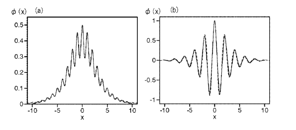
Figure 1: Typical examples of numerically found and analytically predicted (solid and dashed curves, respectively) stable zero-velocity solitons in Eq. (2) with attraction, $\sigma=-1$ (a), and repulsione, $\sigma=+1$ (b). The amplitude of the optical-lattice potential is $\varepsilon=5$.

In the example shown in Fig. 1(a), the soliton’s amplitude is $A=0.5$ and its norm is $N=0.354$. In Fig. 1(b), the amplitude is $A=1$, and the norm is $N\equiv 0.873$. In both parts of Fig. 1, the dashed profiles show the analytical predictions (24) and (28), respectively, corresponding to the same values of the amplitude. The comparison with the analytical approximations makes it obvious that they are very accurate in both cases. At other values of the parameters, the agreement between the numerically found and analytically predicted shapes of the solitons is, generally, as good as in these examples.

It is necessary to stress that, alongside broad solitons extending to many periods of the OL, a generic example of which is shown in Fig. 1(a), stable narrow solitons, which are confined, essentially, to a single OL cell, also exist in the attractive model. They were found in Ref. [12]. Quite similarly, the 2D and 3D counterparts of the 1D equation (2) with attraction also support both narrow (“single-cell”) and broad (“multi-cell”) stable solitons [7].

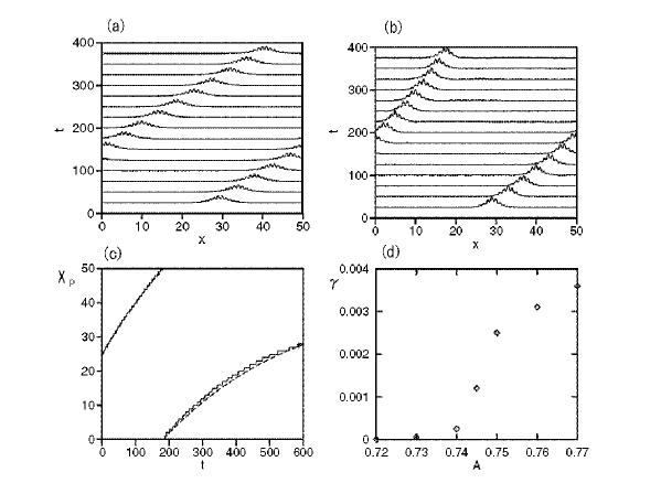
Figure 2: Results of numerical simulations of the moving soliton generated by the initial condition (29) with $k=0.2$. The panels (a) and (b) here, as well as in Figs. 4 and 5 below, and Figs. 6 and 8 show the time evolution of $\left|\phi(x)\right|$. In the panel (a), the initial amplitude of the soliton is $A=0.5$, while panels (b) and (c) pertain to $A=0.75$. The panel (c) displays a relatively early stage of the motion of the soliton’s center in the case of braking, the dashed curve being the fit to Eq. (30). The panel (d) shows the braking rate, defined as in Eq. (30), vs. the soliton’s amplitude.

3.2 Moving solitons in the attractive model

The next step is to simulate moving solitons that were also predicted above. Starting with the attractive model, in Fig. 2 we display a numerically found moving soliton, which is generated, in the attractive model, by the analytical waveform (24) with $\varepsilon=5$,

$$\phi_{0}(x)=A~{}e^{ik(x-L/2)}\left[0.877+0.216\cos\left(2\pi(x-L/2)\right)\right]\,\mathrm{sech}\left(A(x-L/2)\right),$$ (29)

taken as the initial condition for Eq. (2). In this case, periodic boundary condition were used with the spatial period $L=50$ (results of simulations with the parabolic trapping potential will be presented below). The initial wavenumber in Eq. (29) is $k=0.2$; the amplitude is $A=0.5$ in the case shown in Fig. 2(a), and $A=0.75$ in Fig. 2(b) (the value of $k=0.2$ is formally incompatible with the system’s period, $L=50$, but this mismatch plays no practical role, as the soliton’s size, $l_{\mathrm{sol}}$ $\sim A^{-1}$, inside which the phase field carrying the wavenumber was actually created, is much smaller than $L$).

For $A=0.5$, a stable soliton steadily moving at the velocity $v=0.175$ was found in the simulations, see Fig. 2(a) (the velocity was identified as that of the soliton’s peak). Following Eq. (19), the effective mass corresponding to it was calculated as $k/v$, with the wavenumber $k$ of the initial configuration (29). The thus found effective mass $1.143$ is very close to the analytical value $1.13$ produced by Eq. (23).

For $A=0.75$, the simulations produce an altogether different result: the soliton’s velocity slowly decreases with time, see Figs. 2(b) and 2(c). At a relatively early stage of the evolution, the time dependence of the velocity may be well fitted by

$$v(t)=v_{0}\exp(-\gamma t),\,\mathrm{~{}with}\,v_{0}=0.17,\gamma=0.0025.$$ (30)

To illustrate this, the law of motion $X_{p}(t)=25+0.17(\left[1-\exp(-0.0025t)\right]/0.0025$, which is the temporal integration of Eq. (30), is depicted in Fig. 2(c) by a dashed curve, and the actual trajectory of the soliton’s center is shown by a continuous line.

Figure 2(d) displays the braking rate $\gamma$, which is defined as in Eq. (30), i.e., by fitting the initial law of motion to the exponential decay of the velocity, as a function of the soliton’s amplitude $A$. This dependence was obtained from systematic simulations of Eq. (2) with the fixed OL strength, $\varepsilon=5$, and different initial conditions. The braking sets in at the critical value of the amplitude, $A_{\mathrm{cr}}=0.72$. It is relevant to mention that a qualitatively similar effect was observed, in various forms, in simulations of the motion of a discrete soliton in the NLS lattice equation: if the amplitude of the moving soliton exceeds a critical value, it quickly gets trapped by the lattice [17], otherwise it moves freely [16].

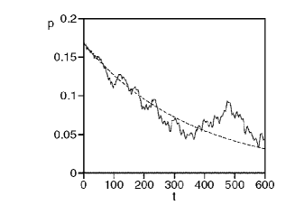
Figure 3: The decay of the soliton’s momentum, in the same case as shown in Figs. 2(b) and 2(c), on a longer time scale. The dashed curve is the fit to Eq. (30).

At a later stage of the evolution, the soliton’s motion law strongly deviates from the exponential relaxation assumed in Eq. (30). To illustrate this, in Fig. 3 we display the evolution of the soliton’s momentum per atom, which is computed from the numerical data as $p=i\int_{-\infty}^{+\infty}\left(\partial\phi^{\ast}/\partial x\right)\phi(x)dx/\int_{-\infty}^{\infty}|\phi(x)|^{2}dx$ [cf. Eq. (8)], at a moderately long time scale. The initial exponential decay, $p(t)\approx 0.168\exp(-0.0028t)$, with the decay rate very close to that in Eq. (30), changes into an erratic motion at a later stage, with the deceleration sometimes changed by acceleration. This picture suggests that dynamical chaos may develop in the motion of the soliton. To further investigate the issue, in Fig. 4 we display continuation of the motion to extremely long time. The figure, and, especially, the continuous power spectrum in panel (c) clearly demonstrate that chaotic motion sets in indeed. However, the soliton’s shape remains strictly coherent at all times, hence that the mean-field approximation based on the GP equation remains relevant in this case, unlike situations when the wave field as a whole becomes chaotic, and the BEC disintegrates, making the GP equation irrelevant [22].

Figure 4: The continuation of the Fig. 3 to an extremely long time scale. The panels (a) and (b) display the time dependences of the coordinate of the soliton’s center and momentum per atom, and the panel (c) is the power spectrum of the latter in the double-logarithmic scale.

3.3 Relaxation of a two-soliton in the attractive model

It is well known that the usual self-focusing NLS equation, i.e., Eq. (2) with $\sigma=-1$ and $\varepsilon=0$, gives rise not only to fundamental solitons, but also to their higher-order counterparts, the simplest one being the two-soliton (a breather), which is generated by the initial condition with the double amplitude. We simulated evolution of similar configurations in the presence of the OL potential, taking, for example, the initial condition as in Eq. (29) but with the amplitude $2A$ instead of $A$ [while $\mathrm{sech}\left(A(x-L/2)\right)$ was not altered]. If the amplitude is smaller than some critical value, this configuration indeed evolves into a persistent breather, see an example in Fig. 5(a) for $A=0.16$. However, a “heavier” initial two-soliton configuration relaxes into a stationary fundamental soliton, like in Fig. 5(b) in the case of $A=0.3$. Figure 5(c) additionally displays the evolution of the pulse’s amplitude in the latter case.

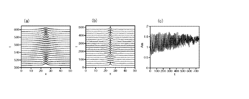
Figure 5: Evolution of the two-soliton, initiated by the initial configuration (29) with the double amplitude: (a) $A=0.16$; (b) and (c): $A=0.3$. A persistent breather appears in the former case, while in the latter case the pulse relaxes (without conspicuous radiation loss) into a fundamental soliton.

It is relevant to mention that the attractive model with the OL potential may have stable static two-soliton (or multi-soliton) solutions of a different type, when two narrow solitons are trapped in two adjacent wells of the OL potential. Such states and their stability limits were found in Ref. [12] in terms of a nonlinear-optical model.

3.4 Moving solitons in the repulsive model

Motion of solitons in the repulsive GP equation (2), with $\sigma=+1$ , was systematically investigated too. Again fixing $\varepsilon=5$, we take, as a generic example, the initial condition in the form suggested by the analytical approximation (28), i.e.,

$$\phi_{0}(x)=1.985~{}A~{}e^{ik(x-L/2)}\cos\left(\pi(x-L/2)\right)\mathrm{sech}\left(A(x-L/2)\right),$$ (31)

cf. Eq. (29). The outcome of the simulation, corresponding to $k=0.1$ in Eq. (31), is shown in Fig. 6, which displays the evolution of $\left|\phi(x)\right|$ for two different amplitudes, (a) $A=0.30$ and (b) $A=0.55$. In the former case, the gap soliton moves steadily at the velocity $v=-0.274$. The effective mass corresponding to this soliton, as determined from the numerical data according to the same definition as above, $m_{\mathrm{eff}}=k/v$, is $-0.365$, which is close enough to the analytical value $-0.34$ produced by Eq. (27).

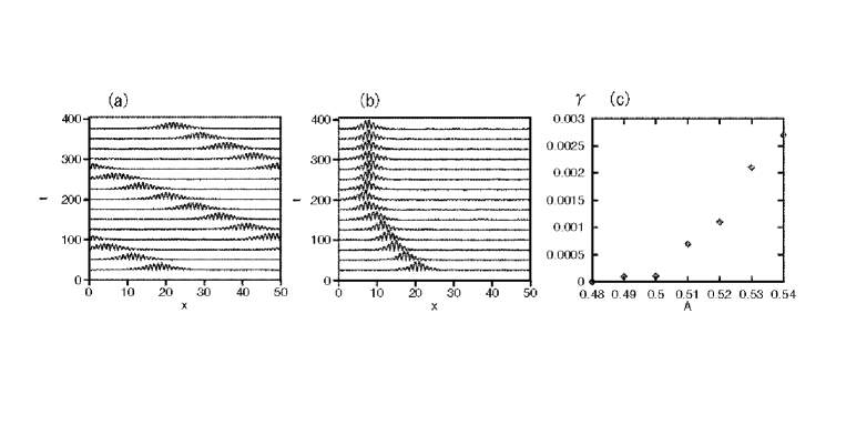
Figure 6: The panels (a), (b) and (c) show the same as (a), (b) and (d) in Fig. 2, but for the case when the soliton is launched in the repulsive model, using the initial condition (31) with $k=0.1$. The panels (a) and (b) correspond to the amplitudes $A=0.30$ and $0.55$, respectively.

Figure 6(b) shows that a heavier soliton, with $A=0.55$, does not move steadily. Instead, it starts to brake, like heavy solitons in the attractive model, see Fig. 2. The velocity decays exponentially at the initial stage of the evolution, like in Eq. (30), the corresponding damping rate $\gamma$ being displayed in Fig. 6(c) versus $A$. As well as in the attractive model, the transition from the steady motion to the braking occurs at a critical value of the soliton’s amplitude, which is $A_{\mathrm{\ cr}}\approx 0.48$ in this case.

4 Solitons in the parabolic trap or anti-trap

Any experimental setup in BEC uses a parabolic trap [15] (bright 1D solitons were observed in an expulsive potential created by an inverted trap [2]). This means that the underlying GP equation (2) should be extended to the form

$$i\frac{\partial\phi}{\partial t}=-\frac{1}{2}\frac{\partial^{2}\phi}{\partial x^{2}}+\left[\sigma|\phi|^{2}-\varepsilon\cos\left(2\pi x\right)+B\left(x-\frac{L}{2}\right)^{2}\right]\phi,$$ (32)

where $B$ is the strength of the trap, and its center is set at $x=L/2$.

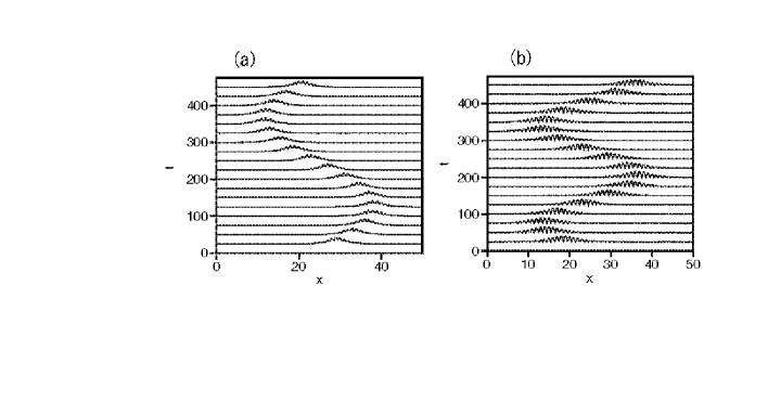
Figure 7: Motion of the soliton in the weak parabolic potential: (a) the trap with $B=0.0001$; (b) the inverted potential (anti-trap) with $B=-0.0001$. The strength of the optical lattice is $\varepsilon=5$. In the cases shown in (a) and (b), the solitons were set in motion by lending them the initial velocities $v_{0}=0.172$ and $-0.270$, respectively.

Figure 7(a) shows the evolution of $\ \left|\phi(x)\right|$ in the attractive model ($\sigma=-1$) with $\varepsilon=5$ and a weak trap, $B=0.0001$, as obtained from numerical simulations of Eq. (32). The initial condition is again taken in the form of Eq. (29), which is suggested by the analytical approximation (24), with $A=0.5$ and $k=0.2$. In this case, the soliton performs harmonic oscillations in the trap, and the motion of the soliton’s center-of-mass coordinate, which we define as

$$X_{p}(t)\equiv\int_{-\infty}^{\infty}x|\Phi|^{2}dx/\int_{-\infty}^{\infty}|\Phi|^{2}dx,$$ (33)

is well approximated by the expression

$$X_{p}(t)=25+13\sin(0.0132~{}t).$$ (34)

To proceed with an analytical approach to the soliton’s motion in the parabolic potential, we insert the same ansatz (16), which was used above, into Eq. (32), and derive a modified version of Eq. (17),

$$i\Phi_{t}=-\left(1/2\right)m_{\mathrm{eff}}\Phi_{xx}+\left[\sigma g|\Phi|^{2}+B(x-L/2)^{2}\right]\Phi.$$ (35)

Then, the following relation is an exact corollary of Eq. (35),

$$m_{\mathrm{eff}}\ddot{X}_{p}=-2B(X_{p}-L/2),$$ (36)

where the overdot stands for the time derivative. In the model with attraction, where the effective mass is positive, Eq. (36) predicts harmonic oscillations of the soliton with the frequency $\omega_{\mathrm{ho}}=\sqrt{2B/m_{\mathrm{eff}}}$. For instance, in the example shown in Fig. 7(a), Eq. (23) with $\varepsilon=5$ yields $m_{\mathrm{eff}}=1.13$, hence, with $B=0.0001$, we predict the frequency $\omega_{\mathrm{ho}}=0.0133$, which is to be compared with the numerically found value $\omega_{\mathrm{\ num}}=0.0132$ in Eq. (34).

Figure 7(b) shows the evolution of $|\phi(x)|$ in the repulsive model with the inverted parabolic potential, $B=-0.0001$. The initial condition is again taken in the form of Eq. (31), with $A=0.3$ and $k=0.1$. It is clearly observed that the negative-mass soliton is trapped by the anti-trapping potential. The motion of the soliton’s center is fitted by

$$X_{p}(t)=25-11.5\sin(0.0235~{}t),$$ (37)

cf. Eq. (34). In this case, the analytical approximation (27) with $\varepsilon=5$ yields $m_{\mathrm{eff}}=-0.339$, hence the corresponding harmonic-oscillation frequency with $B=-0.0001$ is $\omega_{\mathrm{ho}}=\sqrt{2B/m_{\mathrm{eff}}}=\allowbreak 0.0243$, which is close to the numerically found value $\omega_{\mathrm{num}}$ that appears in Eq. (37).

We have checked too that, in the case of the usual trap ($B>0$), the negative-mass soliton in the repulsive model is indeed expelled from the trap region, as it should be expected. In that case, its observed motion again complies well with Eq. (36).

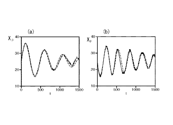
Figure 8: Numerically found trajectories of the soliton’s center in the presence of the harmonic trap or anti-trap, in the case when the soliton’s amplitude exceeds the braking threshold. The GP equation (32) was simulated, with $\sigma=-1$ and $B=0.001$ (attraction and normal trap) in (a), and with $\sigma=+1$ and $B=-0.001$ (repulsion and anti-trap) in (b). The dashed curves show the respective analytical fits (38) and (39).

Lastly, we have also found that, as well as in the absence of the parabolic potential (see above), the motion of the soliton is subject to braking if its amplitude is too large. In that case, the positive- and negative-mass solitons perform damped oscillations in the trapping or anti-trapping potential, respectively. Typical examples are shown in Fig. 8, which displays the motion of the soliton’s center as found from the simulations initiated by the same initial conditions (29) and (31) as above, but with larger amplitudes: $A=0.75$ in (a), and $A=0.52$ in (b). In these two cases, the damped oscillations are well approximated by analytical expressions

$$X_{p}(t)=25+12.5\sin(0.0132t)\exp(-0.0010~{}t)$$ (38)

[the dashed curve in Fig. 8 (a)], and

$$X_{p}(t)=25-10\sin(0.0202~{}t)\exp(-0.0006~{}t)$$ (39)

[the dashed curve in Fig. 8 (b)].

At other values of the parameters, the motion of the positive- and negative-mass solitons in the trapping and anti-trapping potentials is the same as shown in the above examples. In all the cases when the braking did not set in, the numerically simulated motion (both oscillations and expulsion, depending on the signs of the effective mass and the potential) was found to be in good agreement with the predictions based on Eq. (36).

The trapping of the gap soliton by the inverted parabolic potential in the repulsive BEC loaded into an OL is a challenge for experimental verification. We stress that, while the gap soliton should be trapped by the inverted potential, this is definitely not expected for a plain broad distribution of the atomic density, in which case the anti-trapping potential will try to expel atoms in the usual way (of course, this trend may be countered by trapping the atoms in the OL). Thus, the trapping in the inverted parabolic potential is a specifically nonlinear dynamical effect, endemic to the negative-mass solitons.

5 Collisions between oscillating solitons

If the direct or inverted parabolic potential retains the solitons, it is quite easy to create an initial configuration with two well-separated identical solitons, and lend them opposite initial velocities (or just zero velocities, see below). Then, they will start to oscillate in opposite directions, and will thus have to collide periodically. This setting is quite convenient to test the character of collisions between solitons.

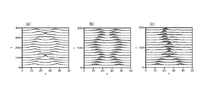
Figure 9: Collisions between positive-mass (a) and negative-mass (b,c) solitons which oscillate, respectively, in the trapping or anti-trapping parabolic potential with the strength $B=\pm 0.0001$. The difference between the cases shown in (b) and (c) is in the initial phase difference $\Delta\varphi_{0}$ between the negative-mass solitons: $\Delta\varphi_{0}=\pi$ in (b), and $\Delta\varphi_{0}=0$ in (c).

We simulated this situation in the attractive model, creating an initial configuration $\phi_{0}(x)$ which was a linear superposition of the analytical approximations (24) for two solitons. As a typical example, in Fig. 9(a) we display the case when centers of the two solitons with equal amplitudes $A=0.3$ are set at the points $x_{1}=L/2-13$ and $x_{2}=L/2+13$, so that

$$\phi_{0}(x) = A\left\{\left[0.877+0.216\cos 2\pi(x-x_{1})\right]\mathrm{sech}\left(A(x-x_{1})\right)\right.$$ (40)

$$+\left.\left[0.877+0.216\cos 2\pi(x-x_{2})\right]\mathrm{sech}\left(A(x-x_{2})\right)\right\}.$$

Note that the initial wavenumbers in this expression are set equal to zero [cf. Eq. (29)], hence the initial velocities of the two solitons are zero too; however, being in-phase, the solitons attract each other, which initiates their oscillatory motion. Figure 9(a) clearly demonstrates (which is also corroborated by extending the simulations to much longer times) that the positive-mass solitons collide repeatedly, each time passing through each other, and remain completely stable.

A typical example of a gap-soliton pair that survives indefinitely many collisions in the repulsive BEC placed in the inverted parabolic potential is displayed in Fig. 9(b). The two solitons were initially taken as a linear superposition of two analytical waveforms (28), again with equal amplitudes $A=0.3$, centers placed at the points $x_{1}=L/2-13$ and $x_{2}=L/2+13$, and zero initial wavenumbers:

$$\phi_{0}(x)=1.985A\left[\cos\left(\pi(x-x_{1})\right)\mathrm{sech}\left(A(x-x_{1})\right)-\cos\left(\pi(x-x_{2})\right)\mathrm{sech}\left(A(x-x_{2})\right)\right].$$ (41)

Unlike the initial condition (29) which was used in the attractive model, the initial phase difference between the solitons in the configuration (40) is $\Delta\varphi_{0}=\pi$, hence they repel each other. In this case too, the solitons perform indefinitely many oscillations, colliding repeatedly without developing any instability. Note that, in contrast with the case shown in Fig. 9(a), this time the colliding solitons do not pass through each other, but rather bounce, which is explained by the fact that they keep the phase difference $\pi$.

However, the solitons do not always collide elastically. Another generic outcome is fusion of two in-phase solitons into a single one. For example, in the repulsive model with the anti-trapping parabolic potential and the same initial configuration as in Eq. (41), but this time with $\Delta\varphi_{0}=0$,

$$\phi_{0}(x)=1.985A\left[\cos\left(\pi(x-x_{1})\right)\mathrm{sech}\left(A(x-x_{1})\right)+\cos\left(\pi(x-x_{2})\right)\mathrm{sech}\left(A(x-x_{2})\right)\right],$$

we have found that the first collision leads to merger of the solitons into one pulse, which is accompanied by some radiation loss, see Fig. 9(c). The resultant single soliton then performs harmonic oscillations with a small amplitude. Qualitatively, the fusion may be explained the following way: in the course of the collision, overlapping between the in-phase solitons leads to increase of the amplitude past the threshold at which the braking sets in (see above).

Further simulations demonstrate that, in the case shown in Figs. 9(b) and 9(c), the colliding solitons eventually merge into one if the initial phase difference between them belongs to the interval $\left|\Delta\varphi_{0}\right|\leq 0.8\pi$. It is noteworthy that, when $\Delta\varphi_{0}$ is close to the critical value ($0.8\pi$, in this example), the fusion happens after several collisions.

In the attractive model, the merger induced by the collisions was observed too, if the solitons’ amplitude was large enough. On the other hand, in both models (repulsive and attractive) merger of solitons with $\Delta\varphi_{0}=\pi$ has not been observed. We stress that (as well as in the case of the discrete NLS equation [17]) solitons with very large amplitudes cannot collide at all, as they will be quickly halted by the braking force induced by the OL.

6 Conclusion

In this work, we aimed to investigate, in a systematic way, motion of 1D solitons in the attractive and repulsive Bose-Einstein condensates (BECs) loaded into an optical lattice (OL) and subject to the action of an external parabolic potential. First of all, we have demonstrated, in two different analytical forms, that, in the repulsive BEC, when the soliton is of the gap type, its effective mass is negative. This gives rise to the prediction that calls for experimental verification: in the latter case, the soliton cannot be confined by the usual trapping parabolic potential, but it can be held by the anti-trapping inverted potential. We have also investigated the motion of the solitons in long systems, concluding that, in both cases of the positive and negative mass, the soliton moves unhindered if its amplitude is below a certain threshold; above the threshold, the soliton is braked by its interaction with the OL. At a late stage of the braking, the damped motion becomes chaotic.

We have also investigated the evolution of the two-soliton state in the attractive model. It was found that the two-soliton generates a persistent breather, if its amplitude is not too large; otherwise, the two-soliton suffers fusion into a single fundamental soliton.

Lastly, we have considered collisions of two solitons trapped in the parabolic potential. Depending on their amplitudes and phase difference $\Delta\varphi$, the solitons perform stable oscillations, colliding indefinitely many times, or they merge into a single soliton, after one or several collisions. However, the merger does not occur in the case of $\Delta\varphi=\pi$.

As concerns values of physical parameters at which the phenomena predicted in this work can be observed in the experiment, they are not different from those for which other soliton effects in OLs were recently predicted [6, 9] (the number of atoms in the soliton may be in the range of $10^{3}-10^{4}$, the number of the OL periods inside the parabolic trap or anti-trap can easily be $\sim 100$ or larger, etc.). Thus, the observation of the gap-soliton’s confinement in the anti-trapping potential and other dynamical phenomena predicted in this work seems quite feasible. Besides that, all the predictions may also be translated into those for solitons in nonlinear photonic crystals. In particular, the capture of the gap soliton by the inverted potential implies that a stable bright optical soliton is possible in a self-defocusing nonlinear anti-waveguide, with the refractive index periodically modulated in the transverse direction.

Results reported in this paper can be extended to the two-dimensional (2D) case. In particular, we have demonstrated that a 2D gap soliton in a repulsive BEC loaded in a 2D optical lattice may be trapped by an inverted isotropic harmonic potential. In that case, the trapped soliton demonstrates various modes of stable motion, including oscillations with periodic passage through the center, and circular motion around the center. These results will be reported in detail elsewhere.

References

- [1] Han D J, DePue M T and Weiss D S 2001 Phys. Rev. A 63 023405; Burger S, Cataliotti F S, Fort C, Maddaloni P, Minardi F and Inguscio M 2002 Europhys. Lett. 57 1; Denschlag J H, Simsarian J E, Haffner H, McKenzie C, Browaeys A, Cho D, Helmerson K, Rolston S L and Phillips W D 2002 J. Phys. B 35 3095; Greiner M, Mandel O, Hansch T W and Bloch I 2002 Nature 419 51; Morsch O, Cristiani M, Muller J H, Ciampini D and Arimondo E 2002 Phys. Rev. A 66 021601; 2003 Laser Phys. 13 594; Cataliotti F S, Fallani L, Ferlaino F, Fort C, Maddaloni P and Inguscio M 2003 J. Opt. B 5 S17; 2003 New J. Phys. 5 71; Bloch I, Greiner M, Mandel O and T.W. Hansch T W 2003 Phil. Trans. Roy. Soc. L., Ser. A 361 1409.
- [2] Khaykovich L, Schreck F, Ferrari G, Bourdel T, Cubizolles J, Carr L D, Castin Y and Salomon C 2002 Science 296, 1290; Strecker K E, Partridge G B, Truscott A G and Hulet R G 2002 Nature 417 150; 2003 New J. Phys. 5 73.
- [3] Anker Th, Albiez M, Eiermann B, Taglieber M, and Oberthaler M K 2004 e-print cond-mat/0401165.
- [4] V. Ahufinger, A. Sanpera, P. Pedri, L. Santos, and M. Lewenstein, e-print cond-mat/0310042.
- [5] Baizakov B B, Konotop V V and Salerno M 2002 J. Phys. B 35 5105.
- [6] Konotop V V and Salerno M 2002 Phys. Rev. A 65 021602; Louis P J Y, Ostrovskaya E A, Savage C M, and Kivshar Y S 2003 Phys. Rev. A 67 013602; Ostrovskaya E A and Kivshar Y S 2003 Phys. Rev. Lett. 90 160407.
- [7] Baizakov B B, Malomed B A, and Salerno M 2003 Europhys. Lett. 63 642.
- [8] Yang J and Musslimani Z H 2003 Opt. Lett. 28 2094.
- [9] Carusotto I, Embriaco D and La Rocca G C 2002 Phys. Rev. A 65 053611; Hilligsoe K M, Oberthaler M K and Marzlin K P 2002 ibid. A 66 063605; Kevrekidis P G, Frantzeskakis D J, Malomed B A, Bishop A R and Kevrekidis I G 2003 New J. Phys. 5 64; Scott R G, Martin A M, Fromhold T M, Bujkiewicz S, F.W. Sheard and Leadbeater M 2003 Phys. Rev. Lett. 90 110404; Efremidis N K and Christodoulides D N 2003 Phys. Rev. A 67 063608.
- [10] Abdullaev F Kh and Galimzyanov R 2003 J. Phys. B 36 1099.
- [11] Xi P, Zhang Z-Q and Zhang X 2003 Phys. Rev. E 67 026607.
- [12] Malomed B A, Wang Z H, Chu P L, and Peng G D 1999 J. Opt. Soc. Am. B 16 1197.
- [13] Dziarmaga J, Karkuszewski Z P and Sacha K 2002 Phys. Rev. A 66 043615; Dziarmaga J and Sacha K 2002 ibid. 66 043620; Law C K 2003 ibid. 68 015602.
- [14] Bergé L 1998 Phys. Rep. 303 260.
- [15] Dalfovo F, Giorgini S, Pitaevskii L P and Stringari S 1999 Rev. Mod. Phys. 71 463.
- [16] Feddersen H, , in: Nonlinear Coherent Structures in Physics and Biology, ed. by M. Remoissenet and M. Peyrard (Springer-Verlag: Berlin, 1991), p. 159; see also: Duncan D B, Eilbeck J C, Feddersen H and Wattis J A D 1993 Physica D 68 1; Feddersen H 1993 Phys. Scripta 47 481.
- [17] Papacharalampous I E, Kevrekidis P G, Malomed B A and Frantzeskakis D J 2003 Phys. Rev. E 68 046604.
- [18] Eiermann B, Treutlein P, Anker T, Albiez M, Taglieber M, Marzlin K P and Oberthaler M K 2003, Phys. Rev. Lett. 91 060402.
- [19] Gisin B V and Hardy A A 1995 Opt. Quant. Electr. 27 565.
- [20] Olshanii M 1998 Phys. Rev. Lett. 81 938; Pérez-García V M, Michinel H and Herrero H 1998 Phys. Rev. A 57 3837; Salasnich L, Parola A and Reatto L 2002 ibid. A 65 043614; Band Y B, Towers I, and Malomed B A 2003 ibid. A 67 023602.
- [21] de Sterke C M and Sipe J E 1994 Progr. Opt. 33 203.
- [22] Castin Y and Dum R 1997 Phys. Rev. Lett. 79 355; Gardiner S A, Jaksch D, Dum R, Cirac J I and Zoller P 2000, Phys. Rev. A 62 023612; Gardiner S A 2002, J. Mod. Opt. 49 1971.