Anomalous scaling and universality in hydrodynamic systems with power-law forcing

Abstract

The problem of the interplay between normal and anomalous scaling in turbulent systems stirred by a random forcing with a power law spectrum is addressed. We consider both linear and nonlinear systems. As for the linear case, we study passive scalars advected by a $2d$ velocity field in the inverse cascade regime. For the nonlinear case, we review a recent investigation of $3d$ Navier-Stokes turbulence, and we present new quantitative results for shell models of turbulence. We show that to get firm statements is necessary to reach considerably high resolutions due to the presence of unavoidable subleading terms affecting all correlation functions. All findings support universality of anomalous scaling for the small scale fluctuations.

1 Introduction

The understanding of the small scale statistics of turbulent systems is a problem of considerable interest [1]. With turbulent systems, we mean both the dynamics of velocity fields in high-Reynolds number flows, and the advection of scalar or vector fields by turbulent flows as, e.g., temperature or magnetic fields. In the last few years, much progress has been reached both in experimental [2, 3, 4, 5] and numerical [6, 7] investigations of turbulent systems. We have now plenty of observations showing that two properties generally holds. First, turbulent systems are intermittent [1, 8, 5], as quantified by the anomalous scaling of moments of field increments. Second, the anomalous scaling exponents display universality with respect to the boundary conditions and to the large scale forcing mechanisms [8, 9]. Some subtle points arise when isotropy is broken at large scale by the injection mechanisms [10, 5, 11, 12]. In that case, for universality to hold it is required that anisotropic contributions are subleading with respect to the isotropic one. However, evidences for universality of both isotropic and anisotropic scaling exponents have been found [13, 14].

Nonetheless, the mechanisms responsible for anomalous scaling and universality in turbulent systems are still not fully comprehended with the remarkable exception of linear problems such as the passive transport of a field, for which intermittency and universality have been systematically understood (see Ref. [16] for an exhaustive review). In this context, in particular for the class of Kraichnan models [15], closed equations for the correlation functions can be derived. These are linear partial differential equations, whose homogeneous solutions (zero modes) generally exhibit anomalous scaling. On the other hand, the inhomogeneous solutions, constrained by the external forcing, possess dimensional (non-anomalous) scaling. Universality results then from the decoupling between the zero modes scaling and the forcing. Remarkably, the zero modes can be interpreted as statistically preserved structures, i.e. functions that do not change in time once averaged over the velocity field realisations and particle trajectories. This allowed for successfully testing the entire picture also for the advection by realistic velocity fields [17, 18], and in the context of shell models for passive transport [19].

On the theoretical side, it is tempting to export the concepts issuing from linear turbulent systems to nonlinear ones, i.e. to see whether the same mechanisms for anomalous scaling and universality are at work also in nonlinear hydrodynamic systems such as Navier-Stokes turbulence. A possible test case to probe universality with respect to the forcing mechanisms is to study turbulent fluctuations stirred at all scales by a self-similar power-law random forcing. Indeed, the non-analytical properties of the forcing may alter the energy exchange between the turbulent field fluctuations. For instance, in some cases, the energy injection mechanism may prevail over the energy cascade process, modifying the inertial range physics.

This problem was pioneered by means of Renormalisation Group (RG) methods [20, 21, 22], in the late ’70s, for the $d$-dimensional Navier-Stokes equations. In the RG calculations, for $d=3$, the forcing spectrum is chosen as $E_{f}(k)\sim k^{3-y}$ with $y$ playing the role of a small parameter in perturbative expansions. Unfortunately the interesting physical case, obtained for $y=4$ and corresponding to the Kolmogorov spectrum for the velocity field, lies in a range where convergence of the RG expansion is not granted [25]. Notwithstanding extensions of the RG formalism to $y\sim O(1)$ values have been tempted by different approaches [23, 24], the problem is still open. Recent numerical simulations tried to shed light on this issue [26, 27] but, because of the limited resolution, their results are not conclusive.

The aim of this paper is to investigate the general issue of the small scale statistical properties of linear and nonlinear hydro-dynamical systems, in the presence of stirring acting at all scales with a power-law spectrum. A systematic study of the scaling behaviour at varying the forcing spectrum allows indeed for understanding the interplay of dimensional and anomalous scaling in turbulent fields.

In Sec. 2, as an instance of linear problems, we consider passive scalars stirred at all scales by a power-law forcing, and advected by a $2d$ turbulent velocity field. Our results confirm the universality scenario originating from the zero modes picture which predicts two distinct regimes. Forcing-dominated regime: the scaling of low order structure functions is non-anomalous, with exponents dimensionally related to the forcing spectrum; for the higher order moments, scaling is anomalous and dominated by the zero modes. Forcing-subleading regime: the dimensional scaling related to the balance with the forcing is subleading, at any order, with respect to the anomalous one, similarly to the case of a standard large scale injection. Hence, anomalous scaling is observed for any order statistics. A subtle technical point revealed by the passive scalar case is the existence of many important power-law terms that contribute to the scaling properties. As clarified in Sec. 2, for both regimes, to disentangle the authentic scaling behaviours, it is necessary to take into account the leading as well as the subleading terms. Concerning nonlinear systems, in Sec. 3, we review the numerical study of the $3d$ Navier-Stokes equations done in Ref. [27], where due to natural limitation in the resolution only semi-quantitative results were obtained. Then, to overcome this difficulty, we consider shell models for turbulence. These are nonlinear models that maintain most of the richness of the original problem but allow for reaching higher Reynolds numbers. Shell model results coherently fit with the passive scalar and NS ones. Conclusions follow in Sec. 4.

2 Linear dynamics: passive scalar transport

The evolution of a passive scalar field $\theta$ advected by an incompressible flow ${\bm{v}}$ is governed by the advection-diffusion equation :

$$\partial_{t}\theta\,+\,{\bm{v}}\cdot{\bm{\nabla}}\,\theta\,=\,\kappa\,\Delta\,\theta\,+\,f\,,$$ (1)

where $\kappa$ is the molecular diffusivity. The standard phenomenology is as follows. Scalar fluctuations are injected at large scale by the source term $f$; then, by a cascade mechanism induced by the advection term, they reach small scales where dissipation takes place balancing the input, and holding the system in a statistically stationary state.

Since the problem is passive, it can be studied also with a synthetic velocity field mimicking some of the features of realistic turbulent flows. Much attention has been recently devoted to the Kraichnan model [15], where ${\bm{v}}$ is a Gaussian, incompressible, homogeneous, isotropic and $\delta$-correlated in time field of zero mean. The only reminiscence of real turbulent flows is the existence of a scaling behaviour that, due to the assumed self-similarity, is fixed by a unique exponent, i.e. $\langle(\delta_{r}{\bm{v}}\cdot\hat{\bm{r}})^{2}\rangle\sim r^{\xi}$ with $0<\xi<2$ (where $\delta_{r}{\bm{v}}={\bm{v}}({\bm{x}}+{\bm{r}})-{\bm{v}}({\bm{x}})$). For the sake of analytical control, the forcing $f$ is also taken as a Gaussian, homogeneous, isotropic field of zero mean and with correlation function: $\langle f({\bm{r}},t)f({\bm{0}},0)\rangle=\delta(t){\cal F}(r)$, where ${\cal F}(r)$ decays rapidly for $r\gg L_{f}$, identifying $L_{f}$ as the large scale of the problem.

Thanks to the above simplifying assumptions, a closed equation for the generic $p$-point correlator, $C_{p}({\bm{r}},t)=\langle\theta({\bm{r}}_{1},t)\theta({\bm{r}}_{2},t)...\theta({\bm{r}}_{p},t)\rangle$, can be derived. It formally reads

$$\partial_{t}C_{p}=-{\cal M}_{p}C_{p}+{\cal F}\otimes C_{p-2}\,,$$ (2)

where ${\cal F}$ is the forcing spatial correlation defined above, and ${\cal M}_{p}$ is a linear differential operator coming from the diffusion and the advection terms (see Ref. [16] for details). The stationary solution of (2) satisfies the equation ${\cal M}_{p}C_{p}={\cal F}\otimes C_{p-2}$. As usual, a linear equation is solved by the superposition of the solution of the associated homogeneous equation, ${\cal M}_{p}{\cal Z}_{p}=0$, and the solution of the inhomogeneous one, which will be denoted as $C_{p}^{\cal I}$. In the inertial range of scales both $C_{p}^{\cal I}$ and ${\cal Z}_{p}$ display a scaling behaviour, i.e.

$$C_{p}^{\cal I}(\lambda\underline{\bm{r}})\sim\lambda^{\zeta^{dim}_{p}}C_{p}^{\cal I}(\underline{\bm{r}})\qquad{\mbox{and}}\qquad{\cal Z}_{p}(\lambda\underline{\bm{r}})\sim\lambda^{\zeta_{p}}{\cal Z}_{p}(\underline{\bm{r}})\,,\qquad{\mbox{with}}\;\underline{\bm{r}}=({\bm{r}}_{1},\dots,{\bm{r}}_{p})\,,$$ (3)

where the scaling exponents $\zeta_{p}^{dim}=p(2-\xi)/2$ are fixed by dimensionally matching the inertial operator with the forcing, while the $\zeta_{p}$, not constrained by any dimensional requirements, are independent of the forcing. One is usually interested in the $p$-point irreducible component of the correlation function, $C_{p}$, that is the structure function $S_{p}(r)=\langle(\delta_{r}\theta)^{p}\rangle$. Still in the framework of Kraichnan model, the zero modes scaling exponents contributing to $S_{p}$ have been calculated perturbatively in [28, 29]. It has been found that $\zeta_{p}<\zeta_{p}^{dim}$ for $p>2$, i.e. the leading contribution to the structure function scaling is anomalous.

The zero modes dominance scenario explains both the anomalous scaling exponents and their universality. Indeed the forcing does not enter the definition of ${\cal Z}_{p}$, but fixes only the multiplicative constants in front of $C^{\cal I}_{p}$ and ${\cal Z}_{p}$, necessary to match the large scale boundary conditions. This implies that, even though scaling exponents are universal, probability density functions (PDF) of scalar increments are not. The above picture based on zero modes is now recognised to apply in all linear hydrodynamic problems. As confirmed by investigations of passive advection by realistic velocity fields [18, 17], and of shell models for passive transport [19].

Let us now focus on the main issue of this work: the scaling behaviour in the presence of forcing fluctuations directly injected in the inertial range of scales. We consider the case of a source term $f({\bm{r}},t)$ which is a random Gaussian scalar field, with zero mean, white-in-time and characterised by the spectrum

$$E_{f}(k)=\pi k\langle|f({\bm{k}})|^{2}\rangle\propto k^{-1+\beta}\,.$$ (4)

In the following, it is always assumed the presence of ultraviolet and infrared cutoffs for the forcing, i.e. expression (4) holds only in the range $k_{1}\,<\,|{\bm{k}}|\,<\,k_{2}$ of wave-numbers, where $k_{1}$ and $k_{2}$ are of the order of the inverse of the largest scale in the system and of the dissipative scale, respectively.

Remaining in the framework of the Kraichnan model, Eq. (2) still holds, and its stationary solution is again the superposition of the homogeneous solution, ${\cal Z}_{p}$, which remains unchanged (viz. with the same scaling exponents) and of the inhomogeneous one, $C^{\cal I}_{p}$, whose scaling exponents now depend on the slope of the forcing spectrum, $\beta$. Indeed by dimensional reasoning, we have $\zeta_{p}^{dim}(\beta)=p(2-\xi-\beta)/2$.

Two regimes can be identified. If $\beta<0$, the scaling of the inhomogeneous solution is always subleading with respect to the anomalous one. The scaling exponents measured from the structure functions are the same as those obtained with the standard large scale forcing. On the other hand, for $\beta>0$, there exists a critical order $p_{c}$ such that for $p<p_{c}$: $\zeta_{p}^{dim}(\beta)\leq\zeta_{p}$, and for $p>p_{c}$: $\zeta_{p}\leq\zeta_{p}^{dim}(\beta)$. In other words, the scaling behaviour of the low-order structure functions is non-anomalous and dominated by the forcing. The appearing of anomalous scaling for $p>p_{c}$ can be understood due the fact that $\zeta_{p}$ as a function of $p$ is concave. Moreover, it is known numerically [18] and to some degree analytically [30] that in the Kraichnan model the scaling exponents above a certain order saturate to a finite value, $\zeta_{\infty}$, which makes even more intuitive the existence of a finite $p_{c}$. Some subtle points may arise for positive $\beta$ larger than $1$. In such a case, the strong UV components of the forcing spectrum may allow a matching with zero modes, disregarded for a large scale forcing [32], exploding at small scales. Finally, the case $\beta=0$ is marginal, because the exponents $\zeta_{p}^{dim}$ coincide with the large scale prediction, up to possible logarithmic corrections.

Checking the validity of the above predictions in numerical simulations of a realistic flow is interesting for two reasons. First, it is a further demonstration, in the Eulerian framework, of the zero modes picture for anomalous scaling and universality in linear problems, which was previously assayed with Lagrangian studies [17]. Second, it offers a controlled testing ground for interpreting some aspects of the nonlinear hydrodynamics which will be considered in the next section.

As an example of realistic velocity field, we consider two-dimensional incompressible Navier-Stokes equations in the inverse cascade regime [33, 7, 34]:

$$\partial_{t}{\bm{v}}+{\bm{v}}\cdot{\bm{\nabla}}\,{\bm{v}}=-{\bm{\nabla}}P+\eta\Delta{\bm{v}}-\alpha{\bm{v}}+{\bm{f}}_{v}\,.$$ (5)

The terms in the r.h.s. of Eq. (5) have the following meaning: $P$ is the pressure field; ${\bm{f}}_{v}$ injects kinetic energy at scale $L_{0}$; $\nu\Delta{\bm{v}}$ (where $\nu$ is the viscosity) dissipates enstrophy at small scale; $-\alpha{\bm{v}}$ removes energy at the large scales allowing for a statistically stationary state. In the inverse energy cascade regime, the velocity statistics is self-similar (not-intermittent), with $\langle(\delta_{r}{\bm{v}}\cdot\hat{\bm{r}})^{p}\rangle\sim r^{p/3}$, but temporal correlations are non trivial. Moreover, precise numerical measurements of passive scalars with large scale forcing [18, 17] have shown that: $\zeta_{2}=2/3$ while for $p>2$ the exponents are anomalous, and saturation is observed for $p\geq 10$ with $\zeta_{\infty}\simeq 1.4$. It is noteworthy that saturation seems to be generic in passive scalars, as found also in experiments [31]. From a physical point of view, it means that the strongest scalar fluctuations are statistically dominated by front-like structures, i.e. huge variations of the field $\theta$ at very small scales.

Once a power law forcing (4) is considered, the predicted dimensional scaling is $\zeta_{p}^{dim}(\beta)=p(2/3-\beta)/2$. Therefore, the two above described regimes –statistics dominated by zero modes or by the forcing– should appear for $\beta<0$ and $\beta>0$, respectively.

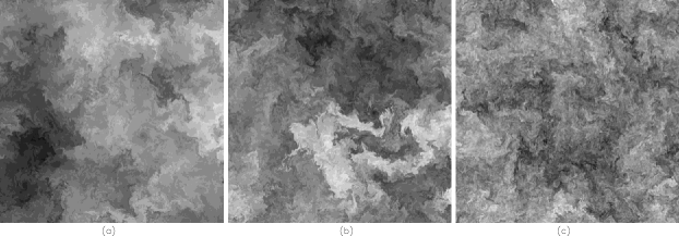
Figure 1: Instantaneous snapshots of the scalar field $\theta$ for runs (a), (b), and (c); intensities are coded in grey-scale. Note that (a) and (b) are qualitatively very similar, while (c) is characterised by richer fluctuations at the small scales. The three snapshots are obtained by integrating Eqs. (1) and (5) by means of a standard $2/3$-dealiased pseudospectral code in a doubly periodic square domain $2\pi\times 2\pi$ with $1024^{2}$ grid points. As for the velocity field, in Eq. (5) the viscous term has been replaced by a hyper-viscous term of order $8$, in order to force at the very small scales. The velocity forcing ${\bm{f}}_{v}$ is chosen as a Gaussian, incompressible, homogeneous, isotropic and $\delta$-correlated in time $2d$ field, of zero mean and concentrated around the small scale $L_{0}$ (of the order of few grid points). The friction coefficient $\alpha$ is tuned in such a way that energy is removed at a scale $\eta_{fr}\sim\epsilon_{v}^{1/2}\alpha^{-3/2}$ of the order of the box size. In Eq. (1), to have a large inertial range, the diffusive term has been replaced by a bilaplacian with $\kappa$ tuned to have the dissipative scale $r_{d}\geq L_{0}$. As for the scalar, in run (a) we used a white-in-time, random Gaussian forcing concentrated at scale $L_{f}$ of the order of the box size. In the runs (b) and (c) we used the forcing (4) by choosing $k_{1}=2$ and $k_{2}$ in such a way that $k_{2}\leq 2\pi/r_{d}$. For the sake of comparison, we imposed in all runs the same scalar energy input. For each run, we collected $80$ frames separated by about one large scale eddy turnover time measured as $\eta_{fr}/\sqrt{\langle v^{2}\rangle}$. See [7, 18] for more details on the numerical procedure.

We performed three sets of direct numerical simulations (DNS) of Eqs. (1),(5): for run (a), we used a standard large scale forcing; for runs (b) and (c), we considered a forcing as in Eq. (4) with $\beta=-0.3$ and $\beta=0.3$, respectively. More details on the DNS are given in the caption of Fig. 1, where we show the snapshots of the scalar field $\theta$ for all runs. Already at a first sight, it is possible to observe that runs (a) and (b), where the zero modes dominate over the inhomogeneous solutions at any order, display qualitatively similar features: the field is organised into large scale structures or plateaux characterised by a good mixing, separated by sharp fronts. Differently in run (c), which corresponds to the case of forcing dominated statistics (with $p_{c}\geq 6$), the scalar fluctuations develop a wider range of scales, and the most evident large scales plateaux disappear.

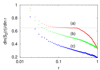
Figure 2: Log-lin plot of local slopes of the second order structure function for the three runs. The dotted straight line indicates the value $2/3$. Note that in run (a) the slope are constant for about one decade. On the other hand, the slopes for run (b) and (c) are non constant in the entire range. It is worth remarking that for power-law forcing there are two sources of finite size effects. The first is the presence of two power-laws, see text. The second is that the scaling in real space of the forcing two-point correlation is strongly affected by corrections (induced by the Bessel function) due to fact that we generate the forcing in Fourier space.

In order to make the above observations more quantitative, we studied the scaling of the structure functions $S_{2p}(r)=\langle(\delta_{r}\theta)^{2p}\rangle$ (odd orders are zero due to the isotropy of the forcing). For run (a), we found a very good scaling range of about one decade, which allowed us for accurately measuring $\zeta_{p}$ up to $p\approx 10-12$. The quality of the local slopes and the measured values agree with previous investigations [18], which were performed with larger statistics and higher resolution. For the power-law cases, runs (b) and (c), we could not find evidence of a good scaling as in run (a). This is observed already from the second order structure function $S_{2}$, whose local slope is plotted in Fig. 2 for the three runs.

We understand the poor scaling behaviour as due to the competition between the scaling of the anomalous part and the forcing dominated one. This becomes clear by looking at the scalar flux, $\Pi_{\theta}(r)\equiv\langle[\delta_{r}{\bm{v}}\cdot\hat{\bm{r}}](\delta_{r}\theta)^{2}\rangle$. For this quantity under rather general hypothesis, an exact analytical prediction can be derived for a generic forcing, through the Yaglom equation [35]. For a power law forcing $f$ as in (4), we obtain:

$$\Pi_{\theta}(r)\equiv\langle[\delta_{r}{\bm{v}}\cdot\hat{\bm{r}}](\delta_{r}\theta)^{2}\rangle\sim c_{1}r+c_{2}r^{1-\beta}\,,$$ (6)

where we have kept only the first two leading contributions. It is important to notice that constants $c_{1}$ and $c_{2}$, which depend on the space dimension and on the details of the forcing spectrum, turn out to have opposite signs. In (6), in addition to the standard linear term, there is the first leading term induced by the forcing (4). As one can see, the critical value $\beta=0$ naturally arises in the flux expression to separate the inertial dominated ($\beta<0$) from the forcing dominated ($\beta>0$) regime. Indeed, for $\beta<0$ the spectral flux is dominated by the low wavenumber components of the forcing spectrum and saturates, in Fourier space, to a constant value as a function of $k$. Scalar fluctuations are transferred down-scale via an intermittent cascade and the statistics is dominated by the anomalous scaling, the forcing contribution even if present at all scales is subleading. For $\beta>0$, the scalar spectral flux no longer saturates to a constant: the direct input of energy from the forcing mechanism affects inertial range statistics in a self-similar way, down to the smallest scales where dissipative terms start to be important.

In addition to $\Pi_{\theta}(r)$, we also studied the third moment of the flux variable $\Pi^{3}_{\theta}(r)=\langle[(\delta_{r}{\bm{v}}\cdot\hat{\bm{r}})(\delta_{r}\theta)^{2}]^{3}\rangle$ whose scaling is anomalous for the large-scale forcing case, i.e. $\Pi^{3}_{\theta}(r)\sim r^{2.4}$ (see also [18]). Results are summarised in Fig. 3.

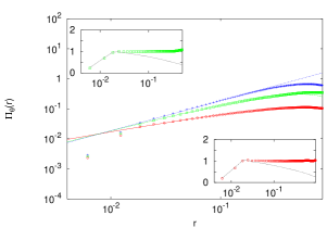
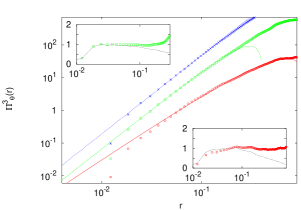
Figure 3: Left: structure functions of passive scalar flux variables. Blue crosses: run (a); green squares: run (b); red circles: run (c). Fits are made in the inertial range with the expression given by the Yaglom equation (6). Insets: same analysis is performed for compensated ratios in the case of run (b) (top inset) and run (c) (bottom inset). We show the best compensation obtained with both power laws (same symbols as in the body of the figure) in Eq. (6), and with only the leading term (dotted lines). Right: the same of left panel for the third order moment of the flux variable. For the large scale forcing we use the single power-law, $r^{2.4}$, to fit the data, while for the other two cases we used a power law superposition of the two terms of Eq. (7). For all fits with a power-law superposition, the two terms turns out to have opposite signs. Insets: compensations with a single (leading) or two power laws for run (b) (top inset) and run (c) (bottom inset). Here also the best compensation is obtained with two power laws.

Concerning the flux $\Pi_{\theta}(r)$, for the large scale case run (a), the scaling is good and the Yaglom relation, $\Pi_{\theta}(r)\approx-2\epsilon_{\theta}r$ (being $\epsilon_{\theta}$ the scalar dissipation), holds for about one decade (Fig. 3, left panel). On the other hand, for the power-law forced cases, the scaling is poorer, making the identification of the exponents less trivial. Indeed, a scaling behaviour can be properly identified only by taking into account both the leading and subleading terms in Eq. (6). The third order moment is affected by the same problem. So that, on the basis of relation obtained for $\Pi_{\theta}$, we tried to fit it with the following scaling ansatz:

$$\Pi^{3}_{\theta}(r)\sim Ar^{2.4}+Br^{3(1-\beta)},$$ (7)

where the exponent $2.4$ in the first term is associated to the anomalous contribution as measured from run (a). Notice that for run (b) the exponent induced by the forcing is subleading, i.e. $3(1-\beta)=3.9$, while for run (c) it becomes leading $3(1-\beta)=2.1$. From the insets of Fig. 3, it is clear that a well defined scaling behaviour is recovered only after having taken into account the two power-law contributions. In all cases the anomalous scaling exponents have values in agreement with those obtained for a large scale forcing, although the interplay of different power laws, when the the forcing is as (4), makes the identification of the exponents very difficult even at considerably high resolution.

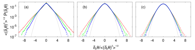
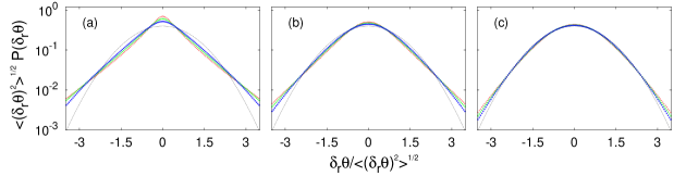
Figure 4: Top: PDF of scalar increments, $\delta_{r}\theta$, for runs (a), (b) and (c). For each run, we plot the PDF for three different separations $r$ inside the inertial range. The curves have been normalised to have unit variance. The dotted line is a Gaussian distribution with unit variance for comparison. Bottom: the same but zooming in, to highlight the core behaviour. Note that for run (c) the PDF’s core approaches a Gaussian with a weaker, if not absent, dependence of $r$.

Due to these difficulties in measuring the exponents, we looked directly at the PDF of scalar increments $P(\delta_{r}\theta)$. In Fig. 4, we show plots of normalised PDFs of $\delta_{r}\theta$ for different choices of the scale $r$ in the inertial range. For runs (a) and (b), the PDFs do not display any rescaling property at changing the scale $r$, neither in the core nor in the tails, suggesting intermittent behaviour in the full statistics. Note also that the PDFs in the two runs are different (only scaling exponents are universal while PDFs are not). Conversely, for run (c), where the forcing is dominant, the PDFs display a fairly good rescaling in the core (which governs the low order statistics), while the tails still do not collapse. This agrees with the existence of a critical order, $p_{c}$, above which anomalous scaling appears even in the forcing-dominated case.

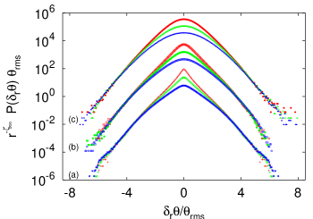
Figure 5: PDF of scalar increments rescaled to test Eq. (8) with $\zeta_{\infty}\simeq 1.4$ for all runs (a), (b) and (c). For plotting purposes, curves of runs (b) and (c) have been shifted by a factor $10^{3}$ and $10^{6}$, respectively.

As discussed earlier, all differences associated with the two regimes should disappear in the high order statistics, i.e. for $p>p_{c}$ when anomalous scaling exponents imposed by the zero modes should show up irrespectively of the forcing. In testing this point, the presence of saturation for large $p$ comes into help, indeed it entails that, for large excursions, the PDFs must approach the form [18]:

$$P(\delta_{r}\theta)=r^{\zeta_{\infty}}Q\left(\frac{\delta_{r}\theta}{\theta_{rms}}\right)\frac{1}{\theta_{rms}},$$ (8)

with $\theta_{rms}=\sqrt{\langle\theta^{2}\rangle}$ and $\zeta_{\infty}\simeq 1.4$. Such a prediction is tested and confirmed by the collapse in the PDF tails shown in Fig. 5, which tells us that $\zeta_{\infty}$ is asymptotically approached independently of the forcing.

The above results provide support to the validity of the zero modes picture beyond the boundaries of the Kraichnan model and in agreement with the Lagrangian investigations [17].

3 Nonlinear systems

Observations from the linear problem strongly indicate that the notions of anomalous scaling and universality are closely linked. When we enter the nonlinear world, we do not have any longer a reference theory. Here, we shall rather formulate some working hypothesis suggested by the results from the linear systems and verify their consistency with two cases studied, namely: $3d$ Navier-Stokes turbulence, reviewing the work first presented in [27], and shell models [36] for turbulence.

3.1 The $3d$ Navier-Stokes problem

In the $3d$ case, we consider random forcing defined by a two-point correlation function that in Fourier space reads

$$\langle f_{i}({\bm{k}},t)f_{j}({\bm{k}}^{\prime},t^{\prime})\rangle\propto k^{1-y}P_{ij}({\bm{k}})\delta({\bm{k}}+{\bm{k}}^{\prime})\,\delta(t-t^{\prime})\,,$$ (9)

where $P_{ij}({\bm{k}})$ is the projector assuring incompressibility and the forcing spectrum behaves as $E_{f}(k)\sim k^{3-y}$. Hereafter, we use the definition $y=4-\beta$, referring to the classical notation of the problem as introduced in [20, 21]. Correspondingly, the critical value $\beta=0$, separating the two regimes in the linear case, is now $y_{c}=4$.

The relative importance of the stirring on the small scales can be varied by tuning the slope value $y$ from $y\sim 0$ (meaning strong input at all scales) to $y\rightarrow\infty$ (corresponding to a quasi large scale forcing). Also in NS turbulence, a physical insight can be taken from the behaviour of the energy flux, which is constant through scales up to logarithmic corrections for the subleading forcing case, $y>y_{c}$; while it becomes a scale dependent function for $y<y_{c}$, overcoming the energy cascade mechanism.

The case of strong input at all scales, $y\sim 0$, was originally investigated in Ref. [20] by means of a RG approach, leading to the following expression for the energy spectrum $E(k)\sim k^{1-2y/3}$, in the domain $\eta\ll k^{-1}\ll L_{f}$ where $\eta$ and $L_{f}$ are the viscous scale and large scale of the system, respectively. It is worth noticing that such a prediction, which results also from dimensional analysis [22], leads to the Kolmogorov spectrum $E(k)\sim k^{-5/3}$ for $y=4$, i.e. quite far from the perturbative region where the RG calculations are under control. Here we want to study the same problems addressed for the linear case, i.e. whether fluctuations are sensitive to the injection mechanism for any $y$ and if one observes anomalous scaling for $y<4$, when the forcing is dominant. Since, at least with the present knowledge, RG perturbative methods starting at $y\sim 0$ cannot control anomalous corrections, only numerical simulations at finite $y$ values, can possibly give some answers.

In Ref. [26] a first numerical investigation of $3d$ incompressible Navier-Stokes problem was performed. The authors made a set of DNS, varying the spectrum slope from $y=3$ to $y=8$ at low Taylor’s Reynolds number $Re_{\lambda}=22$. Without considering the issue of anomalous scaling in the region $y\,<\,y_{c}=4$, they mostly concentrated on the cases with $y\geq 4$, and ended up with the conclusion that for $y\geq 4$ the properties of the statistics are not universal, but varies with the forcing spectrum slope. It is however difficult to consider these as conclusive results, because of the large error bars affecting the data. Later, in Ref. [27], another numerical study of the same problem at a much higher resolution (up to $Re_{\lambda}=220$) has given some support, even if mostly based on semi-quantitative results, to the scenario drawn in the previous section in the context of passive transport.

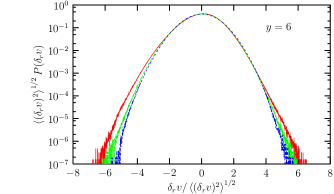
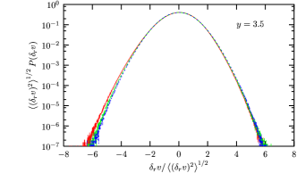
Figure 6: Left: PDF of the velocity increments, for $y=6.0$, for three separations $r_{1}=34\eta$ and $r_{2}=74\eta$ in the inertial range, and $r_{3}=114\eta$ in the energy containing range. Distributions are normalised to have unit variance. Right: the same as in the left panel, but for the case $y=3.5$. The incompressible Navier-Stokes equations are solved with a second-order hyper-viscous dissipative term $\propto\nu\Delta^{2}$. Temporal integration has been carried over for about $20-30$ large-eddy turnover times. DNS data refer to $256^{3}$ simulations. The range of the forcing, in Fourier space, extends down to the maximum resolved wavenumber.

In particular, we report here the behaviour of longitudinal velocity increments PDFs for two among the different runs done in [27], with $y=3.5$ and $y=6$. For $y=6>y_{c}$, as shown in Fig. 6 left panel, the usual intermittent behaviour for the PDFs is found: the curves $P(\delta_{r}v)$ at different separations $r$ do not rescale one onto the other. On the contrary, for $y=3.5<y_{c}$, the PDFs at various scales are almost indistinguishable (see Fig. 6, right panel): a signature of the absence of intermittent corrections at least for the core of the distribution. It is worth noticing that this result is far from trivial, because it coincides with the RG predictions [20, 21, 22, 23, 24] in the region where RG calculations are well beyond their range of validity. These findings, even if qualitative, fit rather well with those of the passive scalar case (see Fig. 4).

We may try to push forward this indication in the light of the theory for linear systems. For the $3d$ Navier-Stokes dynamics, the stationary equations for multi-point correlators ${\cal C}_{p}({{\bm{r}}},t)\equiv\langle v_{\alpha_{1}}({\bm{r}}_{1})v_{\alpha_{2}}({\bm{r}}_{2})\ldots v_{\alpha_{p}}({\bm{r}}_{p})\rangle$ can be sketched as,

$$\Gamma_{p+1}\,{\cal C}_{p+1}+\nu\,D_{p}\,{\cal C}_{p}+{\cal F}_{2}{\cal C}_{p-2}=0,$$ (10)

where $\Gamma_{p+1}$ is the integro-differential linear operator coming from the inertial and pressure terms, $D_{p}$ is the differential operator describing dissipative effects and ${\cal F}_{2}$ is the two-point forcing correlator. Unfortunately, since the hierarchy (10) is unclosed, no straight-forward analytical approache can be done. Even though nothing can be rigorously said, one may still be tempted to assume that anomalous scaling is brought by the inertial operator. However, the presence of finite size effects, due to the limited inertial range, in DNS data of $3d$ Navier-Stokes simulations [27] provide only a semi-quantitative support to this scenario. As we shall see in the next section, more quantitative statements can be made in the context of shell models for turbulence, for which resolution constraints are much less severe.

3.2 Shell models for turbulence

Shell models of turbulence are dynamical systems mimicking Navier-Stokes nonlinear evolution [36]. Their main advantage relies on the possibility of performing high Reynolds number simulations to measure statistical properties, say intermittent corrections, with high accuracy. The model we use, proposed in [37], is an improved version of the GOY model [38, 39] (see also [40] for a recent review). The evolution equation is :

$$\frac{d}{dt}u_{n}=i(k_{n}u^{*}_{n-2}u_{n-1}+b\,k_{n-1}u^{*}_{n-1}u_{n+1}+(1+b)k_{n-2}u_{n+1}u_{n+2})-\nu k^{2}_{n}u_{n}+f_{n}\,.$$ (11)

The velocity field fluctuation at the wavenumber $k_{n}$, with $k_{n}=2^{n}k_{0}$, is expressed in terms of the complex variable $u_{n}$; $b$ is a free parameter and $\nu$ indicates the viscosity. The number of shells varies as $n=\{0,\dots,N_{max}\}$. Remarkably, for large scale forcing, the structure functions show anomalous scaling:

$$S_{p}(k_{n})\equiv\langle|u_{n}|^{p}\rangle\sim k^{-\zeta_{p}}_{n}$$ (12)

deviating from the dimensional prediction $\zeta_{p}=p/3$. Moreover, anomalous scaling exponents are found to be universal with respect to the forcing, provided it is large scale (see [40]).

We aim at investigating the properties of the model stirred by a white-in-time, Gaussian field, with zero mean and spectrum

$$\langle|f_{n}|^{2}\rangle=f_{0}k^{\beta}_{n},$$ (13)

being $f_{0}$ the forcing intensity. A similar injection mechanism was proposed in [41] where authors tried to compare the power-law forced shell models with fractal-grid induced turbulence [43]. In order to understand the effect of forcing as (13) let us start with the energy flux, which obeys an exact equation. Denoting with $\dot{E}_{N}={d\over{dt}}\sum_{n=0}^{N}\langle{|u_{n}|^{2}}/{2}\rangle$ the time derivative of the energy content up to the scale $N$, the energy balance relation can be written as :

$$\dot{E}_{N}+\nu\sum_{n=0}^{N}k^{2}_{n}\langle|u^{2}_{n}|\rangle=-k_{N}\Pi_{N}+\sum_{n=0}^{N}\langle|f_{n}|^{2}\rangle\,.$$ (14)

In the previous expression, $\Pi_{N}=\langle{\cal T}_{N}\rangle$, where ${\cal T}_{N}$ is the energy flux through the shell $N$ defined as

$${\cal T}_{N}=\Im\left\{u^{*}_{N}u^{*}_{N+1}u_{N+2}+\frac{(1+b)}{2}u^{*}_{N-1}u^{*}_{N}u_{N+1}\right\}\,.$$ (15)

For the forcing (13) and for $\nu\to 0$, we get an exact prediction in the stationary state:

$$\Pi_{n}=A_{1}k^{-1}_{n}+B_{1}k^{-1+\beta}_{n}\,,$$ (16)

where the constants $A_{1},B_{1}$, bound by the equation of motion to have opposite signs, depend on the forcing details ($f_{0}$, $\beta$) and on the integral wavenumber $k_{0}$. At this level, where everything is exact, we see that when $\beta$ approaches the critical value ($\beta=0$), a large number of shells is needed to distinguish leading terms from subleading ones in the third order moment. In our runs, the choice of a large value for $N_{max}(=40)$, allow us to have a good control of such effects.

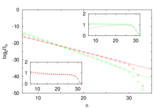
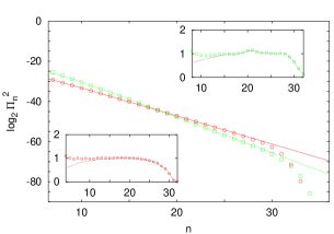
Figure 7: Left: Shell fluxes measured in the presence of a power-law forcing. In our runs, we adopted the following choice of parameters: $b=-0.4$, $\nu=10^{-12}$, $N_{max}=40$. For the random forcing, acting on all shells of the inertial range, we chose the following values of $\beta$: $\beta=0.3$ (green squares), $\beta=-0.15$ (red circles). Fits are made with a superposition of two power-law contributions, in agreement with (16). Insets: compensation with the leading power law (dotted) or with two power laws for $\beta=0.3$ (bottom inset) and $\beta=-0.15$ (top inset). Right: same as left panel but for the second order flux moment, to be compared with (20). Also here the two power laws terms have opposite signs.

Similarly to the NS case (10), we can write the unclosed hierarchy for the multi-point correlators of shell variables:

$$\frac{d}{dt}C_{p}(\underline{n})=M_{p+1}(\underline{n},\underline{n}^{\prime})\,C_{p+1}(\underline{n}^{\prime})+F_{2}(\underline{n},\underline{n}^{\prime})\,C_{p-2}(\underline{n}^{\prime})\,,$$ (17)

where $C_{p}(\underline{n})=\langle u_{n_{1}}u_{n_{2}}...u_{n_{p}}\rangle$ is the generic correlation function of order $p$, $M_{p+1}(\underline{n},\underline{n}^{\prime})$ is the linear operator coming from the inertial terms, and $F_{2}(\underline{n},\underline{n}^{\prime})$ is the two-point forcing operator. The main difference with the case of passive scalar transport, as pointed out in the previous subsection, is that now the system (17) is not closed, i.e. we have more unknowns than equations. Without any ambition of a rigorous approach, we may imagine that the general solution is characterised by two terms. The first, $C^{{\cal I}}_{p}$, given by the dimensional matching between the inertial operator and the forcing operator,

$$M_{p+1}(\underline{n},\underline{n}^{\prime})\,C^{\cal I}_{p+1}(\underline{n}^{\prime})=F_{2}(\underline{n},\underline{n}^{\prime})\,C^{\cal I}_{p-2}(\underline{n}^{\prime}).$$ (18)

The second, ${\cal Z}_{p}$, associated to a “zero mode” of the inertial operator, namely a solution of the homogeneous equation, $M_{p+1}(\underline{n},\underline{n}^{\prime}){\cal Z}_{p+1}(\underline{n}^{\prime})=0\,$. Here, as for the linear problem, the non homogeneous terms are the only contributions depending on the forcing, while the homogeneous ones, dimensionally unconstrained, may show anomalous scaling. In particular, for the structure functions $S_{p}(k_{n})$, we have

$$S_{p}(k_{n})\sim k^{-\zeta_{p}}_{n}+k^{-\zeta^{dim}_{p}(\beta)}_{n}\,,$$ (19)

where $\zeta^{dim}_{p}(\beta)=p/3(1-\beta)$. This implies the following behaviour for the second order moment of the flux (equivalent to the sixth-order structure function):

$$\Pi^{2}_{n}=\langle{\cal T}_{n}^{2}\rangle=A_{2}k^{-1.8}_{n}+B_{2}k^{2/3(\beta-1)}_{n},$$ (20)

where the power $1.8$ coincides with the anomalous exponent measured for sixth-order structure function with a large scale forcing, and the value $2/3(\beta-1)$ comes from the dimensional prediction (18).

In Fig. 7 the first and second moments of the flux variables are shown for both the subleading and dominant forcing with $\beta=-0.15$ and $\beta=0.3$, respectively. It is easy to see that to get a good agreement of the numerical results with the prediction (20), both the leading and the subleading power laws have to be taken into account. For both cases with $\beta=0.3$ and $\beta=-0.15$, at least for the order of the statistics we could reach, the anomalous scaling exponents have values in agreement with those found for a large scale forcing, supporting the universality scenario.

4 Conclusions

We have discussed the problem of small scale fluctuations in turbulent systems stirred at all scales by a power-law forcing. The main question in our study concerns anomalous scaling and universality of scaling exponents.

For linear systems – i.e. passive transport–, we find clear evidence for the universality of anomalous fluctuations and our results fit well in the zero mode scenario. In the regime in which forcing is subleading anomalous scaling is recovered in quantitative agreement with the case of large scale forcing. In the forcing dominated regime, the dimensional scaling imposed by the injection mechanism overwhelms the anomalous fluctuations of low order moments. Nevertheless, anomalous scaling shows up again for high enough moments, independently of the forcing spectrum slope, as confirmed by the existence of a unique saturation exponent in all regimes.

The results obtained for nonlinear turbulent systems point in the same direction. Indeed both the semi-quantitative results obtained in the context of $3d$ Navier-Stokes turbulence and those more quantitative issuing from the investigation of the shell models are compatible with the linear systems scenario for universality. However, in the presence of power-law forcing acting in the turbulent energy cascade range, as shown both in the linear and nonlinear cases, scaling properties are strongly spoiled by the beating of leading and subleading terms. This effect is particularly strong due to cancellations induced by different signed pre-factors in the power-law terms.

Strong cancellation effects, which apparently are a mere technical question, may lead to misinterpretation in analysing data. We wonder, for example, if the observed multi-fractal behaviour in the one-dimensional Burgers equation stirred by a power-law forcing might be a spurious effect [42].

References

References

- [1] Frisch U 1995 Turbulence: The Legacy of A. N. Kolmogorov (Cambridge: Cambridge University Press)
- [2] Noullez A, Wallace G, Lempert W, Miles R B and Frisch U 1997 J. Fluid Mech. 339, 287
- [3] La Porta A, Voth G A, Crawford A M, Alexander J, Bodenschatz E 2001 Nature 409, 1017
- [4] Mordant N, Michel O, Metz P and Pinton J F 2001 Phys. Rev. Lett. 87, 21
- [5] Warhaft Z 2000 Annu. Rev. Fluid Mech. 32, 203
- [6] Gotoh T, Fukayama D and Nakano T 2002 Phys. Fluids 14, 1065
- [7] Boffetta G, Celani A and Vergassola M 2000 Phys. Rev. E 61, R29
- [8] Sreenivasan K R and Antonia R A, 1997 Annu. Rev. Fluid Mech. 29, 435
- [9] Arneodo A, Baudet C, Belin F, Benzi R, Castaing B, et al. 1996 Europhys. Lett. 34, 411
- [10] Arad I, Dhruva B, Kurien S, L’vov V S, Procaccia I and Sreenivasan K R 1998 Phys. Rev. Lett. 81, 5330
- [11] Kurien S and Sreenivasan K R 2000 Phys. Rev. E 62, 2206
- [12] Shen X and Warhaft Z 2002 Phys. Fluids 14, 2432
- [13] Biferale L and Toschi F 2001 Phys. Rev. Lett. 86, 4831
- [14] Biferale L, Calzavarini E, Toschi F and Tripiccione R 2003 Europhys. Lett. 64 461
- [15] Kraichnan R H 1968 Phys. Fluids 11, 945
- [16] Falkovich G, Gawȩdzki K and Vergassola M 2001 Rev. Mod. Phys. 73, 913
- [17] Celani A and Vergassola M 2001 Phys. Rev. Lett. 86, 424
- [18] Celani A, Lanotte A, Mazzino A and Vergassola M 2001 Phys. Fluids 13, 1768
- [19] Arad I, Biferale L, Celani A, Procaccia I and Vergassola M 2001 Phys. Rev. Lett. 87, 164502
- [20] Forster D, Nelson D R and Stephen M J 1997 Phys. Rev. A 16 732
- [21] Frisch U and Fournier J D 1978 Phys. Rev. A 17, 747
- [22] De Dominicis C and Martin P C 1979 Phys. Rev. A 19 419
- [23] Yakhot V and Orszag S A 1986 Phys. Rev. Lett. 57, 1722
- [24] Adzhemyan L Ts, Antonov N V, Kompaniets M V and Vasil’ev A N 2003 Intern. Journ. Modern Physics B 17, 2137
- [25] Eyink G 1994 Phys. Fluids 6, 3063
- [26] Sain A, Manu and Pandit R 1998 Phys. Rev. Lett. 81, 4377
- [27] Biferale L, Lanotte A and Toschi F 2004 Phys. Rev. Lett. to appear; e-Print arXive nlin.CD/0310022
- [28] Gawȩdzki K and Kupiainen A 1995 Phys. Rev. Lett. 75, 3834
- [29] Chertkov M, Falkovich G, Kolokolov I and Lebedev V 1995 Phys. Rev. E 2, 4924
- [30] Balkovsky E and Lebedev V 1998 Phys. Rev. E 58, 5776
- [31] Moisy F, Willaime H, Andersen J S and Tabeling P 2001 Phys. Rev. Lett. 86, 4827
- [32] Bernard D, Gawȩdzki K and Kupiainen A 1998 J. Stat. Phys. 90, 519
- [33] Paret J and Tabeling P 1998 Phys. Fluids 10, 3126
- [34] Tabeling P 2002 Phys. Rep. 362, 1
- [35] Monin A and Yaglom A 1975 Statistical FluidMechanics, Vol.2 (Cambridge: MIT Press)
- [36] Bohr T, Jensen M H, Paladin G and Vulpiani A 1998 Dynamical system approach to turbulence (Cambridge: Cambridge University Press)
- [37] L’vov V S, Podivilov E, Pomyalov A, Procaccia I and Vandembroucq D 1996 Phys. Rev. E 58, 1811
- [38] Yamada M and Ohkitani K 1987 J. Phys. Soc. Jpn. 56, 4210
- [39] Jensen M H, Paladin G and Vulpiani A 1991 Phys. Rev. A 43, 798
- [40] Biferale L 2003 Ann. Rev. Fluid Mech. 35, 441
- [41] Mazzi B, Okkels F and Vassilicos J C 2002 Eur. Phys. J. B 28 243
- [42] Hayot F and Jayaprakash C 1997 Phys. Rev. E 56, 4259
- [43] Staicu A, Mazzi B, Vassilicos J C and van de Water W 2003 Phys. Rev. E 67, 066306