Abstract

We examine a simple, fuel-air, model of combustion in spark ignition (si) engine with indirect injection. In our two fluid model, variations of fuel mass burned in cycle sequences appear due to stochastic fluctuations of a fuel feed amount. We have shown that a small amplitude of these fluctuations affects considerably the stability of a combustion process strongly depending on the quality of air-fulel mixture. The largest influence was found in the limit of a lean combustion. The possible effect of nonlinearities in the combustion process were also discussed.

Keywords: stochastic noise, combustion, engine control

1 Introduction

Cyclic combustion variability, found in 19th century by Clerk (1886) in all spark ignition (si) engines, has attracted great interest of researchers during last years (Heywood 1988, Hu 1996, Daw et al. 1996, 1998, 2000, Wendeker et al. 2003, 2004). Its elimination would give 10% increase in the power output of the engine (Heywood 1988). The key source of their existence may be associated with either stochastic disturbances (Roberts et al. 1997, Wendeker et al. 1999) or nonlinear dynamics (Daw et al 1996, 1998) of the combustion process. Daw et al. (1996, 1998) and more recently Wendeker et al. (2003, 2004) have done the nonlinear analysis of the experimental data of such a process. Changing an advance spark angle they observed the considerable increase of the noise level (Wendeker et al. 2003) claiming that it is due to chaotic dynamics of the process. On the other hand the main sources of cyclic variability were classified by Heywood (1988) as the aerodynamics in the cylinder during combustion, the amount of fuel, air and recycled exhaust gases supplied to the cylinder and a mixture composition near the spark plug. In this paper we will model the variation of fuel ignition amount as the most common source of instability in indirect injection.

The present paper is organized as follows. After the introduction in the present section we define the model by a set of difference equations in the next section (Sec. 2). This model, in deterministic and stochastic forms, will be applied in Sec. 3, where we analyze the oscillations of burned mass. Finally we derive conclusions and remarks in Sec. 4.

2 Two fluid model of fuel-air mixture combustion

Starting from fuel-air mixture we define the time evolution of the corresponding amounts. Namely, we will follow the time histories of the masses of fuel $m_{f}$, and air $m_{a}$.

Table 1: Constants and variables of the model.

stoichiometric coefficient	$s=14.63$
exhaust ratio	$\alpha=0.92$
air mass in a cylinder	$m_{a}$
fuel mass in a cylinder	$m_{f}$
fresh air amount	$\delta m_{a}$
fresh fuel amount	$\delta m_{f}$
air/fuel ratio	$r=m_{a}/m_{f}$
burned fuel mass	$\Delta m_{f}$
combusted air mass	$\Delta m_{a}$
air/fuel equivalence ratio	$\lambda$
random number generator	$N(0,1,i)$
mean value
of fresh fuel amount	$\delta m_{fo}$
standard deviation
of fresh fuel amount	$\sigma_{mf}$
standard deviation
of the equivalence ratio	$\sigma_{\lambda}$

Figure 1: The combustion curve $\Delta m(\lambda)$ for the constant fresh air feed $\delta m_{a}=200$ mg.

Firstly, we assume the initial value of $m_{a}(i)$, $m_{f}(i)$ automatically their ratio $r(i)$:

$$r(i)=\frac{m_{a}(i)}{m_{f}(i)}$$ (1)

for $i=0$.

Secondly, depending on parameter $r$ with reference to a stoichiometric constant $s$ we have two possible cases: fuel and air deficit, respectively. For a deterministic model, the first case lead to

$$r(i)>1/s$$ (2)

we calculate next masses using following difference equations:

$$m_{f}(i+1) = (1-\alpha)\left(m_{f}(i)-\frac{1}{s}m_{a}(i)\right)+\delta m_{f}$$

$$m_{a}(i+1) = \delta m_{f},$$ (3)

where $\alpha$ is the exhaust ratio of the engine, $\delta m_{f}$ and $\delta m_{a}$ denotes fresh fuel and air amounts added in each combustion cycle $i$. In the opposite (to Eq. 2.2) case

$$r(i)<1/s$$ (4)

we use the different formula

$$m_{f}(i+1) = \delta m_{f}$$

$$m_{a}(i+1) = (1-\alpha)\left(m_{a}(i)-sm_{f}(i)\right)+\delta m_{a}$$ (5)

Note that variables $m_{a}$ and $m_{f}$ are the minimal set of our interest. From the above equations one can easily calculate other interesting quantities as the combusted masses of fuel $\Delta m_{f}(i)$ and air $\Delta m_{a}(i)$ and air-fuel equivalence ratio before each combustion event $i$:

$$\lambda\approx s\frac{m_{a}(i)+(1-\alpha)\Delta m_{a}(i-1)}{m_{f}(i)+(1-\alpha)\Delta m_{f}(i-1)}$$ (6)

Basing on experimental results we use the additional necessary condition (Kowalewicz 1984) of combustion process

$$0.6<\lambda<1.3.$$ (7)

For better clarity our notations of system parameters: constants and variables are summarized in Tab. 1.

Basing on the relations (Eqs. 2.1-2.7) we plotted the combustion curve for the assumed constant fresh air feed $\delta m_{a}=200$ mg.

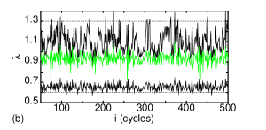
Figure 2: The dependence of $\lambda$ on sequential cycles $i$ for deterministic (a) and stochastic (b) processes. The fresh air amount was assumed to be $\delta m_{a}=200$ mg while the fresh fuel amount varies: $\delta m_{f}=13.50$ mg , 14.63 mg, 21.00 mg starting from the top curve, respectively.

Finally, in the case of stochastic injection, instead of constant $\delta m_{f}(i)$ (Eqs. 2.3 and 2.5) (for each cycle $i$) we introduce its mean value $\delta m_{fo}={\rm const.}$, while $\delta m_{f}$ in the following way:

$$\delta m_{f}(i)=\delta m_{fo}+\sigma_{mf}N(0,1,i),$$ (8)

where $N(0,1,i)$ represents random number generator giving a sequence $i$ of numbers with a unit-standard deviation of normal (Gaussian) distribution and the nodal mean. The scaling factor $\sigma_{mf}$ corresponds to the mean standard deviation of the fuel injection amount. The cyclic variation of $\delta m_{f}(i)$ can be associated with such phenomena as fuel vaporization and fuel-injector variations.

3 Oscillations of burned fuel mass

Here we describe the results of simulations. Using Eqs. 2.1-2.8 we have performed recursive calculations for deterministic and stochastic conditions and obtained time histories of various system parameters: $m_{f}$, $m_{a}$, $\Delta m_{f}$, $\Delta m_{a}$ and $\lambda$. The results for $\lambda$ are shown in Fig. 2. The upper panel (Fig. 2a), corresponding to deterministic combustion for three different values of fuel injection parameter $\delta m_{f}$, shows $\lambda$ as straight lines versus cycle $i$, while the lower (Fig. 2b) one reflects the variations of $\lambda$ in stochastic conditions. The order of curves appearing in the Fig. 2b is the same as in Fig. 2a stating from the smallest value of considered fuel injection amounts from the top. In stochastic simulations we used input of random fuel injection with standard deviation equal to 10% of its mean value $\sigma_{mf}=0.1~{}\delta m_{fo}$. The obtained results clearly indicate that the fluctuations of $\lambda$ are growing with larger $\lambda$. This can be also found by analytical evaluation of Eq. 2.6. It is not difficult to check that

$$\sigma_{\lambda}\sim\lambda^{2}\sigma_{mf}.$$ (9)

Figure 3: The dependence of burned fuel mass on sequential cycles $i$ for deterministic (a) and stochastic (b-d) processes. $\delta m_{a}=200$ mg while $\delta m_{f}$ takes different values: 13.50 mg , 14.63 mg, 21.00 mg denoted in particular figures a-c.

The results for burned fuel mass $\Delta m_{f}$ are presented in Fig. 3. Starting from deterministic conditions ($\delta m_{f}=\delta m_{fo}={\rm const.}$) we obtain the constant fraction of the burned fuel mass $\Delta m_{f}$ represented by the three straight lines in Fig. 3a lying very close to each other. In Fig 3 b-c we show the same, $\Delta m_{f}$, for the considered case of assumed fuel injection ($\delta m_{fo}=13.50$ mg - Fig. 3b, $\delta m_{fo}=14.63$ mg - Fig. 3c, $\delta m_{fo}=21.00$ mg - Fig. 3d) and stochastic conditions. Due to different magnitudes parameter $\lambda$ fluctuations, and dependence of combustion curve Fig. 1 it is not surprise that the fluctuations of $\Delta m_{f}$ have different character in all these cases. For lean combustion, which is a stable process in deterministic case, the fuel injection fluctuations introduce considerable instabilities to the combustion process leading to the suppression of combustion because in some cycles (Fig. 3b) where $\lambda$ is larger that $1.3$. Then Equation 2.7 is not satisfied. In the next case (Fig. 3c) the effect of stochasticity is much smaller. Here we have optimal air-fuel mixture. First of all one should note that fluctuations of $\lambda$ are smaller than in previous case (Fig. 2b). Moreover $\lambda$ oscillate around the region ($\lambda\approx 1$) in combustion curve (Fig. 1) which does not have big changes comparing to previous case. Finally, Fig. 3d shows the sequence of $\Delta m_{f}$ for the large $\delta m_{fo}$ (rich fuel-air mixture). The fluctuations of $\lambda$ are the smallest of all three ones but $\lambda\approx 0.7$ causes suppressions of combustions in some cycles similarly to the case shown in Fig. 3b.

4 Conclusions

In this paper we examined the origin of combusted mass fluctuations. In case of stochastic conditions we have shown that depending on the quality of fuel-air mixture the final effect is different. The worse situation is for lean combustion. The consequences of it can be observed for idle speed regime of engine work. Unstable engine work, interrupted by the cycles without combustion lead to a large increase of fuel use.

Although the presented two component model is very simple it can reflect the underlying nature of engine working conditions. In spite of fact that the model is characterized by the nonlinear transform (Eqs. 2.3, 2.5 and 2.7) similar to logistic one, we have not found any chaotic region. Possibly that such solutions can be found for non realistic model parameters like $\lambda$ and $\alpha$. The other strong limitation was concerned with the sharp edges of combustion curve ($\Delta m_{f}$ versus $\lambda$ Fig.1) modelled by a Heaviside step $\Theta(x)$ function Eq. 2.7. We used such an approximation as a simplest one but modeling with the exponential growth $\exp(-1/x)$ is more realistic and possible. Similar assumptions of the exponential dependence led to chaotic behaviour in papers (Daw et al. 1996, 1998, Wendeker 2003). From a physical point of view mixture gasoline-air is not uniform before ignition and that can cause nonuniform combustion smearing the edges of the combustion curve Fig. 1. Calculations considering this effect are in progress and the results will be reported in a separate future publication.

References

Clerk D., 1886, The gas engine, Longmans, Green & Co., London.

Daw, C.S., Finney, C.E.A., Green Jr.,J.B., Kennel, M.B., Thomas J.F. and Connolly F.T., 1996, A simple model for cyclic variations in a spark-ignition engine, SAE Technical Paper No. 962086.

Daw, C.S., Kennel, M.B., Finney C.E.A., Connolly F.T., 1998 Observing and modelling dynamics in an internal combustion engine, Phys. Rev. E, 57, 2811–2819.

Daw C.S., Finney C.E.A. and Kennel M.B., 2000, Symbolic approach for measuring temporal ”irreversibility”, Phys. Rev. E, 62, 1912–1921.

Heywood JB., 1988, Internal combustion engine fundamentals, McGraw-Hill, New York.

Hu Z., 1996, Nonliner instabilities of combustion processes and cycle-to-cycle variations in spark-ignition engines, SAE Technical Paper No. 961197.

Kowalewicz A., 1984, Combustion Systems of High-Speed Piston I.C. Engines, Studies in Mechanical Science 3, Elsevier, Amsterdam.

Roberts J.B., Peyton-Jones J.C. and Landsborough K.J., 1997, Cylinder pressure variations as a stochastic process, SAE Technical Paper No. 970059.

Wendeker M., Niewczas A. and Hawryluk B., 1999, A stochastic model of the fuel injection of the si engine, SAE Technical Paper No. 00P-172.

Wendeker, M., Czarnigowski, J., Litak, G. and Szabelski, K., 2003, Chaotic combustion in spark ignition engines, Chaos, Solitons & Fractals 18, 805–808.

Wendeker, M., Litak, G., Czarnigowski, J., and Szabelski, K., 2004, Nonperiodic oscillations of pressure in a spark ignition engine, Int. J. Bifurcation and Chaos 14, in press.