Attraction of Spiral Waves by Localized Inhomogeneities with Small-World Connections in Excitable Media

Abstract

Trapping and un-trapping of spiral tips in a two-dimensional homogeneous excitable medium with local small-world connections is studied by numerical simulation. In a homogeneous medium which can be simulated with a lattice of regular neighborhood connections, the spiral wave is in the meandering regime. When changing the topology of a small region from regular connections to small-world connections, the tip of a spiral waves is attracted by the small-world region, where the average path length declines with the introduction of long distant connections. The ”trapped” phenomenon also occurs in regular lattices where the diffusion coefficient of the small region is increased. The above results can be explained by the eikonal equation and the relation between core radius and diffusion coefficient.

I Introduction

Spiral waves are characteristic structures of excitable media that have been observed in many extended systems such as reaction-diffusion media r1 ; zhou1 ; zhou2 , aggregating colonies of slime mold lee , and heart tissues r2 , where they are suspected to play an essential role in cardiac arrhythmia and fibrillation. Sudden cardiac death resulting from ventricular fibrillation is generated from the fragmenting or breakup of spiral waves r3 ; r3-1 ; Leo . Spiral waves are prone to a variety of instabilities ou1 ; ou2 ; ou3 , one of which is meander instability ou4 ; bar1 , where spiral tips follow a hypocycloid trajectory instead of moving around a small circle. Due to Doppler effect, this spiral may undergo a transition from ordered spiral patterns to a state of defect-mediated turbulence ou3 . In the meandering regime, the spiral tips can be made to drift and controlled by external influences r4 or localized inhomogeneities of defects r5 .

After the concept of small-world connections was proposed by Watts and Strogatz r10 , it has quickly attracted much attention because this kind of connections exists commonly in real world, such as in social systems r6 , neural networks r7 and epidemic problems r8 . Different studies show that a little change of the network connections can essentially change the features of a given medium, and plays a very important role in determining the dynamic behavior of a system.

In numerical simulations, a spatially extended system can be approximately regarded as a network consisting of a number of sites connected with certain topology. In this way localized inhomogeneities can be achieved by changing the topology of the network. In heart tissues, pacemakers dominate the dynamics of the travelling wave behavior and control the heart rhythm. We hypothesize that this happens because the characters and the structures of the local cells are different from other cardiac muscle cells. Could a small-world network describe one of the characters of the pacemaker? To answer this question, we changed the widely used regular network in spiral wave study to a small-world network in part of the system to investigate its effects.

In the next section, we study the effect of a local small-world network on the behavior of spiral waves. We show that this special region is a dynamic attractor for spiral tips. In section III, we compare the effect of the small-world network with that of changing diffusion coefficient in the local region, and show that they are equivalent. We give a discussion and conclude our study in the last section.

II The effect of small-world network

The model we used is the two-variable FitzHugh-Nagumo model r9 with local nearest-neighbor couplings in a region of $N_{1}\times N_{2}$:

$${\frac{du_{i,j}}{dt}} {=} {(a-u_{i,j})(u_{i,j}-1)u_{i,j}-v_{i,j}+D_{u}\nabla^{2}u_{i,j}}$$ (1)

$${\frac{dv_{i,j}}{dt}} {=} {\varepsilon(bu_{i,j}-v_{i,j})+D_{v}\nabla^{2}v_{i,j}}$$ (2)

where $i=1,2,...,N_{1}$, $j=1,2,...N_{2}$; $u_{i,j}(t)$ and $v_{i,j}(t)$ is dimensionless excitable variable and recovery variable respectively; $D_{u}$ and $D_{v}$ are diffusion coefficients of the two variables. The Laplacien in the last term can be approximated as:

$$\nabla^{2}u_{i,j}\cong\frac{1}{h^{2}}(u_{i-1,j}+u_{i+1,j}+u_{i,j-1}+u_{i,j+1}-4u_{i,j})$$ (3)

$$\nabla^{2}v_{i,j}\cong\frac{1}{h^{2}}(v_{i-1,j}+v_{i+1,j}+v_{i,j-1}+v_{i,j+1}-4v_{i,j}).$$ (4)

When $0<a<1$, $b\geq 0$, $D_{v}<<D_{u}$, $\epsilon<<1$, the equation describes an excitable medium, which can be regarded as a simplified model for cardiac tissues. In the following discussion, we set the control parameters as follows: $N_{1}=N_{2}=256$, $a=0.1$, $b=1.0$, $\epsilon=0.005$, $D_{u}=0.33$, $D_{v}=0$. No-flux boundary condition is applied in the simulation.

Using vertical gradient distribution initial condition, we first create spiral waves in regular lattices (Fig. 1(a)). In this case, the spiral tip follows a hypocycloid trajectory, showing a typical sign of meandering state ou4 , see Fig. 1(c). We then create a small-world network in a small local region $\Omega$ of a size $N_{s}\cdot N_{s}(N_{s}<<N_{1})$, where the tip of spiral waves locates. The small-world network is created in the following way: With the probability $p_{s}(0\leq p_{s}\leq 1)$, we reconnect every edge in the region $\Omega$ from one of its original vertex to another vertex chosen randomly in the region r10 (see Fig. 1(b)). The change of connections leads to the change of ”diffusion” mode. Supposing node[i][j] is connected with node[$x_{1}$][$y_{1}$], node[$x_{2}$][$y_{2}$], …node [$x_{k}$][$y_{k}$], then the ”diffusion” term in the Eqs (1) (2) becomes:

$$\nabla^{2}u_{i,j}\cong\frac{1}{h^{2}}(u_{x_{1},y_{1}}+u_{x_{2},y_{2}}+...+u_{x_{k},y_{k}}-k\cdot u_{i,j})$$ (5)

$$\nabla^{2}v_{i,j}\cong\frac{1}{h^{2}}(v_{x_{1},y_{1}}+v_{x_{2},y_{2}}+...+v_{x_{k},y_{k}}-k\cdot v_{i,j})$$ (6)

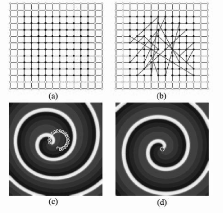
Figure 1: Spiral pattern in different media. (a) a regular network $p_{s}=0$; (b) a small-world network, $p_{s}=0.1$; (c) spiral wave and its tip’s motion in the regular network. the white curve is the trajectory of the spiral tip; (d) spiral wave and its tip’s motion in the small-world network. $N_{s}=10$.

Introducing the small-world network region in the reaction medium greatly influences the motion of the spiral tip. We find that the small-world network region can attract the spiral tip as it passes through the region. After that, the spiral tip rotates around its boundary, as shown in Fig. 1(d). Because the topological structure of the local small-world network is generated randomly under the above mentioned rule, the attraction only occurs under a certain parameter range with certain probability. To characterize the attraction property of the small-world network, we use the attraction probability $p_{a}$ as an order parameter, which can be obtained by repeating (50 times in our work) the simulation using the same control parameters but with different small-world network connections. Our simulation results show that the most influential factor to $p_{a}$ is the small-world creation probability $p_{s}$. As show in Fig. 2(a), $p_{a}$ increases with the increase of the small-world $p_{s}$. When $p_{s}=0$ (corresponding to a regular network), the spiral tip cannot be attracted; when $p_{s}=1$ (corresponding to a random network), the tip can be attracted with probability 1. Between $0<p_{s}<1$, there is a transition where the attraction probability $p_{a}$ increases rapidly. The transition point $p_{c}$ can be defined as the value of $p_{s}$ when $p_{a}=0.5$.

Figure 2: (a) transition curves of $p_{a}$ as a function of $p_{s}$ with different $N_{s}$. The line is the sigmoidal fitting $p_{a}=1-1/(1+\exp((p_{s}-p_{sc})/dp_{s}))$; (b) transition curves of $p_{a}$ as a function of $l$ with different $N_{s}$. The line is the fitting of $p_{a}=1/(1+\exp((l-l_{c})/dl)).$ Here $l_{c}$ is the critical length where $p_{a}=0.5$, and $dl$ is the transition width.

One of the most important characters of small-world network is the reducing of average path length while keeping the clustering coefficient almost constant r10 . Define the normalized average path length $l$ of small-world network as $l=L/L_{0}$, where $L$ is the average path length of small-world network in $\Omega$ r11 and $L_{0}$ is the average path length of regular network in $\Omega$. $l$ will decrease from $1$ to $\varepsilon(\varepsilon>0)$ when $p_{s}$ changes from 0 to 1. From numerical simulations, we find the same type of transition curve of $p_{a}$ as a function of $l$, as shown in Fig. 2(b), indicating that the major effect of the small-world topology to the behavior of spiral waves is the decrease of average path length. In addition, defining the critical length $l_{c}$ as the value of $l$ when $p_{a}=0.5$, we find that the critical length decreases linearly as the increase of the size of $\Omega$, see Fig. 3(a).

III Compare with increasing the diffusion coefficient

Our simulation results suggest that the major effect of the small-world network on spiral tip movement comes from the long distance connections, which lead to shortening the average path length ($l$) and increasing the diffusion speed. If the above suggestion is correct, the phenomenon of spiral tip attraction should also occur when we locally increase the diffusion constant in Eqs. (1) and (2). In this part of work, we increase the diffusion coefficient in a small circular region $\Omega$ by $D$ times and keep the system with regular connections. In the following discussion, we will use $D_{u}^{\Omega}$ to denote the diffusion coefficient in region $\Omega$, and use $D_{u}^{0}$ for the region outside of $\Omega$, so that $D_{u}^{\Omega}=D\cdot D_{u}^{0}$. We find that the spiral tip can be attracted and travel around the boundary of region $\Omega$ when $D$ is large enough and $R>R_{0}$.($R$ is the radius of $\Omega$, $R_{0}$ is the core radius of spiral when $D_{u}^{\Omega}=D_{u}^{0}$). At a given $R$, we can define two values $D_{1}$ and $D_{2}$: A temporal attraction occurs when $D_{1}<D<D_{2}$. In that case, the tip can be trapped for a short period and then escapes; the ”trapped” time increases with $D$. When $D>D_{2}$, the tip can be trapped for a long enough period. Define $D_{c}$ as the mean value of $D_{1}$ and $D_{2}$, the plot of $D_{c}$ with different $R$ is shown in the Fig. 4.

The above simulation results suggest that the increase of diffusion speed in the small region is responsible for the attraction of the spiral tip. To quantitatively compare the two systems, we analyze the diffusion terms of the two systems. In the small-world network, because of the long distance connections, the average distance between nodes declines as $p_{s}$ increases from $0$ to $1$. In a network model of a reaction-diffusion system, this effect can be in a sense translated from the decrease of the average path length between nodes while keeping the distance of two neighboring nodes $h$ constant, to the decrease of the step length $h$ while keeping the network regular. The normalized average path length $l$ can also describe the relative change of $h$. From this argument, the diffusion items of the small-world network can be expressed as:

$$D_{u}^{0}\frac{1}{(lh)^{2}}(u_{i-1,j}+u_{i+1,j}+u_{i,j-1}+u_{i,j+1}-4u_{i,j})$$ (7)

$$D_{v}^{0}\frac{1}{(lh)^{2}}(v_{i-1,j}+v_{i+1,j}+v_{i,j-1}+v_{i,j+1}-4v_{i,j})$$ (8)

At the critical point, for a fixed $R$, the diffusion terms in two systems should be the same. So that $D_{u}^{\Omega}\cdot 1/h^{2}=D_{c}\cdot D_{u}^{0}\cdot 1/h^{2}=D_{u}^{0}\cdot 1/(l_{c}\cdot h)^{2}$, which gives $D_{c}\cdot l_{c}^{2}=1$ . As presented in Fig. 3(b), our simulation fits this analysis within the range of error. This result indicates that our proposition is reasonable. The attracting effect of the small-world network comes from the decline of $l$ inside the inhomogeneous area $\Omega$.

Figure 3: (a) The critical length $l_{c}$ as a function of the region’s radius $R$, $(R=Ns/2)$, the error bar is $dl$,(see the caption of Fig. 2(b) about the fitting); (b) $D_{c}\cdot l_{c}^{2}$ as a function of $R$.

IV Discussion

A question should be answered before fully understanding the effect of the small-world network in the dynamics of spiral tips: what is the mechanism for the spiral tip attraction? In the following discussion, we give an explanation with the eikonal equation, Luther equation Luther , and the relation between diffusion coefficient and of spiral core radius. According to the analysis of the spiral tip dynamics given by Hakim and Karma r13 , for the steady rotational movement of a spiral tip in an excitable medium, the core radius $R$ as a function of diffusion coefficient can be written as:

$$R=\frac{D_{u}}{c_{0}}(\frac{b\cdot K}{B_{c}-\frac{2D_{u}}{W}})^{3/2}$$ (9)

Where $D_{u}$ is the diffusion coefficient of activator ($u$); $c_{0}$ is the speed of plane wave; $b$, $K$ and $B_{c}$ are all constants. $W$ is the constant width of the excited region. In the simulation, We assume that at the boundary of $\Omega$ exists a ”virtual” gradient region of $D_{u}$ which links the outside and inside regions. For a given $R$ of the region $\Omega(R>R_{0}=R(D_{u}^{0}))$, the ”trapped” motion of the spiral tip requires a specific value of $D_{u}$, satisfying equation (9). When $D_{u}<D_{u}^{\Omega}$, the spiral tip will enter the gradient region where the system can find the required $D_{u}$, so that the spiral tip will rotate around the gradient area at the boundary of $\Omega$; on the other hand, when $D_{u}>D_{u}^{\Omega}$, the ”trapped” motion can not be sustained by the central region. From this argument, at critical point, we will have $D_{u}(R)=D_{u}^{\Omega}=D_{c}\cdot D_{u}^{0}$. As shown in Fig. 4, Our simulation results are consistent with this analysis with the range of error.

Figure 4: The critical diffusion coefficient $D_{c}$ as a function of $R$, where the line is the best fitting with Equation (9). The error bars are estimated using $D_{1}$ and $D_{2}$.

To prove the ”trapped” state of tip motion is a stable state, we apply the eikonal equation, which determines the relation between the curvature of a travelling wave front and its speed in an excitable medium, and the Luther relation, which describes the relation between the speed of chemical waves and the diffusion coefficient of activator Luther . the eikonal equation is: $N=C-D_{u}\cdot\kappa$, where $N$ is the normal wave speed, $\kappa$ is the local curvature of the wave front; the Luther equation is: $c=\alpha\cdot\sqrt{D_{u}},$ where $\alpha$ is a constant. Insert the Luther equation into eikonal relation we have:

$$N=\alpha\cdot\sqrt{D_{u}}-D_{u}\cdot\kappa$$ (10)

Taking partial derivative of R in Eq. (10), we get:

$$\frac{\partial N}{\partial R}=[\frac{1}{2}\alpha(D_{u})^{-1/2}-\kappa]\cdot\frac{\partial D_{u}}{\partial R}$$ (11)

At the spiral tip we have $N=0$, so that:

$$\frac{\partial N}{\partial R}\left|{}_{tip}\right.=-\frac{1}{2}\kappa_{tip}\cdot\frac{\partial D_{u}}{\partial R}$$ (12)

In our system, assuming there exists a continuous change of $D_{u}$ at the boundary of region ${\Omega}$, we have $\frac{\partial Du}{\partial R}<0$. Thus the equation (12) indicates that $\frac{\partial N}{\partial R}\left|{}_{tip}\right>0$. That means, if we introduce a small deviation from the ”trapped” motion of the spiral tip, the system will return to the ”trapped” state spontaneously, because we have $N<0$ inside the region $\Omega$, and $N>0$ outside the region $\Omega$.($\hat{n}$ points to the center of ${\Omega}$ region).

In conclusion, we find that in an excitable system local change of topological structure can trap the spiral tip. This ability comes from the increase of diffusion speed. We prove this by increasing the diffusion coefficient. We also give a theoretical explanation using the eikonal equation, Luther equation, and the relation between core radius and diffusion coefficient, which fits well with the results of simulation. We should note that there are other situations where the tip of spiral waves can be trapped in a given area. For example, Lázár et al. reported that self-sustained chemical waves can rotate around a central obstacle in an annular 2-D excitable system, and the wave fronts in the case of an annular excitable region are purely involutes of the central obstacle in the asymptotic state Zolly . Obviously this phenomenon is beyond our analysis. So that more work should be done to fully understand the attract effect of local inhomogeneities in an excitable reaction-diffusion system.

- (1) Electronic address: qi@pku.edu.cn
- (2) A.N. Zakin and A.M. Zhabotinsky, Nature 225, 535 (1970).
- (3) L.Q. Zhou and Q. Ouyang, Phys. Rev. Lett. 85, 1650 (2000).
- (4) L.Q. Zhou and Q. Ouyang, J. Phys. Chem. A 105, 112 (2001).
- (5) K.J. Lee, E.C. Cox, and R.E. Goldstein, Phys. Rev. Lett. 76, 1174 (1996).
- (6) J.M. Davidenko, A.M. Pertsov, R. Salomonz, W. Baxter, and J. Jalife, Nature 335, 349 (1992).
- (7) J.N. Weiss, A. Garfinkel, H.S. Karagueuzian, and P.S. Chen, Circulation 99, 2819 (1999).
- (8) M.L. Riccio, M.L. Koller, and R.F. Gilmour, Circ. Res. 84, 955 (1999).
- (9) L. Glass, Physics Today 8, 40 (1996).
- (10) Q. Ouyang and J.-M. Flesselles, Nature 379, 143 (1996).
- (11) A. Belmonte, J.-M. Flesselles, and Q. Ouyang, Europhys. Lett. 35, 665 (1996).
- (12) Q. Ouyang, H.L. Swinney and G. Li, Phys. Rev. Lett. 84, 1047 (2000).
- (13) G. Li, Q. Ouyang, and H.L. Swinney, Phys. Rev. Lett. 77, 2105 (1996).
- (14) D. Barkley, Phys. Rev. lett. 68, 2090 (1992).
- (15) K.I. Agladze and P. DeKepper, J. Phys. Chem. 96, 5239 (1992).
- (16) S. Nettesheim, A. von Oertzen, H.H. Rotermund, and G. Ertl, J. Chem. Phys. 98, 9977 (1993).
- (17) D.J. Watts and S.H. Strogatz, Nature 393, 440 (1998).
- (18) J.J. Collins and C.C. Chow, Nature 393, 409 (1998).
- (19) J.J. Hopfield and A.V.M. Herz, Proc. Natl. Acad. Sci. U.S.A. 92, 6655 (1995).
- (20) S.A. Pandit and R.E. Amritkar, Phys. Rev. E 60, R1119 (1999).
- (21) R.A. FitzHugh, Biophys. J. 1, 445 (1966).
- (22) R. Albert and A.L. Barabasi, Rev. Mod. Phys. 74, 47 (2002).
- (23) R. Arnold, K. Showalter, and J.J. Tyson, J. Chem. Educ. 64, 740 (1987).
- (24) V. Hakim and A. Karma, Phys. Rev. E 60, 5073 (1999).
- (25) A. Lázár, Z. Nosztizius, H. and Farkas, Chaos, 2, 443 (1995).