Multiplicities of Periodic Orbit Lengths for Non-Arithmetic Models

Abstract

Multiplicities of periodic orbit lengths for non-arithmetic Hecke triangle groups are discussed. It is demonstrated both numerically and analytically that at least for certain groups the mean multiplicity of periodic orbits with exactly the same length increases exponentially with the length. The main ingredient used is the construction of joint distribution of periodic orbits when group matrices are transformed by field isomorphisms. The method can be generalized to other groups for which traces of group matrices are integers of an algebraic field of finite degree.

1 Introduction

For chaotic systems the density of classical periodic orbits with a given length increases exponentially. In particular, for all constant negative curvature surfaces generated by discrete groups one has the universal asymptotics (see e.g. [11])

$$\rho_{\mbox{\scriptsize total}}(l)\stackrel{{\scriptstyle l\to\infty}}{{\longrightarrow}}\frac{e^{l}}{l}\;.$$ (1)

Much less is known about multiplicities of periodic orbits with exactly the same length. Usually it is assumed that the mean length multiplicity of periodic orbits for generic systems depends only on exact symmetries and for models without geometrical symmetries the mean multiplicity $\bar{g}$ equals $2$ or $1$ for systems respectively with or without time-reversal invariance.

Physically it means that, in general, there exists no reason that two different periodic orbits would have the same length except for time-reversal invariant systems where almost all trajectories can be traversed in two opposite directions which implies that $\bar{g}=2$. In semiclassical approach to spectral statistics of chaotic systems the distinction between these two classes of models is reflected in different behaviour of the two-point correlation form factor at the origin which agrees with the predictions of the random matrix theory [1], [2].

For the free motion on constant negative curvature surfaces generated by discrete groups the situation is different. In such hyperbolic models periodic orbits are in one-to-one correspondence with conjugacy classes of group matrices and the length of a periodic orbit, $l_{p}$, is directly related with the trace of a matrix $M$ representing each class (see e.g. [11])

$$|\mbox{Tr}M|=\left\{\begin{array}[]{cl}2\cosh l_{p}/2\;,&\mbox{ if }\det M=1\\ 2\sinh l_{p}/2\;,&\mbox{ if }\det M=-1\end{array}\right.\;.$$ (2)

Hence, any relations between traces of group matrices imply connections between periodic orbit lengths.

The extreme case corresponds to the so-called arithmetic groups (see e.g. [4] and references therein). For such groups traces of group matrices can take only quite restricted set of values and the number of possible traces less than a given value is asymptotically [4]

$$N(|\mbox{Tr}M|<X)\stackrel{{\scriptstyle X\to\infty}}{{\longrightarrow}}CX$$ (3)

with a system dependent constant $C$. Because $X\stackrel{{\scriptstyle l\to\infty}}{{\longrightarrow}}e^{l/2}$ but not all possible values of traces really appear for group matrices, the number of periodic orbits with different lengths when $l_{p}\to\infty$ has the following upper bound [4]

$$N_{\mbox{\scriptsize diff.}}(l_{p}<l)\leq Ce^{l/2}\;.$$ (4)

Define the mean multiplicity of periodic orbit length as the ratio of the density of all periodic orbit to the density of periodic orbits with different lengths

$$\bar{g}(l)=\frac{\rho_{\mbox{\scriptsize total}}(l)}{\rho_{\mbox{\scriptsize diff.}}(l)}$$ (5)

where $\rho_{\mbox{\scriptsize diff.}}(l)=dN_{\mbox{\scriptsize diff.}}(l_{p}<l)/dl$.

From the above formulas one proves [4] that for arithmetic groups the mean multiplicity is exponentially large and has the following estimate from below

$$\bar{g}(l)\geq\frac{2e^{l/2}}{Cl}\;.$$ (6)

In classical mechanics such large multiplicities play a minor role but their interference changes drastically quantum mechanics of arithmetic groups. In particular, spectral statistics of arithmetic systems is close to the Poisson statistics typical for integrable systems and not to the random matrix statistics conjectured for chaotic models [4], [6], [5].

Arithmetic systems are very exceptional but according to the Horowitz–Randol theorem [12], [13] for all hyperbolic models generated by discrete groups multiplicities are unbounded. Nevertheless, multiplicities covered by this theorem are quite rare and a priori assumption would be that for non-arithmetic hyperbolic models the mean multiplicity equals 2 as for generic time-reversal invariant systems.

Numerical calculations performed in [4] indicated that it is not always the case. In that paper certain non-arithmetic Hecke triangles were considered and it was observed that mean multiplicity of periodic orbits with length $l$ seems to increase exponentially

$$\bar{g}(l)\sim e^{\lambda l}$$ (7)

with an exponent $\lambda<1/2$.

The purpose of this paper is two-fold. First, we perform numerical calculations of periodic orbits for much larger lengths that in [4] and, second, we develop a method which gives a lower bound of multiplicities, thus in certain cases confirming analytically exponential growth of multiplicities.

The plan of the paper is the following. In Section 2 we discuss general properties of Hecke triangle group matrices. In Section 3 results of numerical calculations of periodic orbit length multiplicities for a few Hecke triangles are presented. As traces of Hecke triangle group matrices are integers of an algebraic field, each group matrix defines not one but a few different lengths corresponding to different isomorphisms of the basis field. In Section 4 the construction of the joint distribution for periodic orbits with all transformed lengths fixed is discussed. In Section 5 it is demonstrated how the knowledge of this joint distribution permits to calculate the lower bound of the periodic orbit length multiplicity. In Section 5.1 the computations are performed for the simplest case of Hecke groups with $n=5\;,\;8\;,\;10\;,\;12$ which are characterized by the existence of only one non-trivial isomorphism. In Appendix A it is proved that for Hecke triangle groups all transformed lengths are smaller than the true length. This inequality is sufficient to ensure that for Hecke groups with only one non-trivial isomorphism length multiplicities increases exponentially. Our results agree well with direct numerical computations of periodic orbit multiplicity for these groups. In Section 5.2 other Hecke groups are shortly considered. It appears that in all investigated cases except groups with one non-trivial isomorphism length multiplicities increase so slowly that the direct check is practically impossible. In Section 6 we briefly discuss the influence of periodic orbit length multiplicities on the spectral statistics for corresponding systems. In Section 7 a summary of the results is given. In Appendix B a saddle point method of calculation of the joint distribution of periodic orbit lengths is discussed.

2 Hecke triangles

Hecke triangles are hyperbolic triangles with angles $0,\pi/2,\pi/n$ with integer $n\geq 3$. All of them are fundamental regions of discrete groups $G_{n}$ generated by reflections across its sides. Let us denote the reflection across the side connecting angles $0$ and $\pi/2$ by $A$, the one across the side connecting angles $0$ and $\pi/n$ by $B$ and the last one by $C$. From geometrical considerations these transformations obey the defining relations

$$A^{2}=B^{2}=C^{2}=1\;,\;(AC)^{2}=(BC)^{n}=-1\;.$$ (8)

The explicit form of $A$, $B$, and $C$ can be chosen as follows

$$A=\left(\begin{array}[]{cc}-1&0\\ 0&1\end{array}\right)\;,\;B=\left(\begin{array}[]{cc}-1&2\cos\pi/n\\ 0&1\end{array}\right)\;,\;C=\left(\begin{array}[]{cc}0&1\\ 1&0\end{array}\right)\;.$$ (9)

Arbitrary matrix from the Hecke triangle group $G_{n}$ is a word of these letters. Due to (8) these symbols have a complicated grammar. For our purposes it is convenient to introduce new symbols

$$\alpha_{1}^{m} = C(AB)^{m}\;,$$

$$\alpha_{2}^{m} = CB(AB)^{m}\;,$$

$$\alpha_{3}^{m} = CBC(AB)^{m}\;,$$ (10)

$$\ldots \ldots$$

$$\alpha_{n-2}^{m} = \underbrace{CBCB\ldots}_{n-2\;\mbox{\scriptsize symbols}}(AB)^{m}$$

where $m=1,2,\ldots$ are positive integers.

Explicitly up to unessential overall sign

$$\alpha_{2k+1}^{m}=\left(\begin{array}[]{cc}-a_{k}&\alpha ma_{k}+a_{k-1}\\ -a_{k+1}&\alpha ma_{k+1}+a_{k}\end{array}\right),\;\alpha_{2k}^{m}=\left(\begin{array}[]{cc}-a_{k-1}&\alpha ma_{k-1}+a_{k}\\ -a_{k}&\alpha ma_{k}+a_{k+1}\end{array}\right)$$ (11)

where from now we denote

$$\alpha=2\cos\pi/n$$ (12)

and $a_{k}\equiv a_{k}(\alpha)$ are the Chebyshev polynomials of the second kind of $\alpha$

$$a_{k}=\frac{\sin(k\pi/n)}{\sin(\pi/n)}\;.$$ (13)

Using the defining relations (8) one can proves [4] that conjugacy classes in $G_{n}$ (and, consequently, periodic orbits in Hecke triangles) can be constructed as free words in these new symbols with the only restriction that cyclic permutations correspond to the same orbit.

Due to specific form of generators (9) matrix elements of the Hecke triangular group matrices are polynomials with integer coefficients of the variable $\alpha\equiv 2\cos\pi/n$, thus forming naturally a subfield of the cyclotomic field of degree $2n$.

The constant $\alpha$ defined in (12) obeys a polynomial equation $P_{N}(\alpha)=0$ with integer coefficients

$$P_{N}(x)=\prod_{\begin{array}[]{c}k=\mbox{\small odd }\\ (k,n)=1\end{array}}(x-\alpha_{k}(n))=x^{N}+\ldots$$ (14)

where

$$\alpha_{k}(n)=2\cos(\pi k/n)$$ (15)

and the product is taken over all odd integer $k$ coprime with $n$. The total number of such integers and, consequently, the degree of the defining equation is

$$N=\frac{1}{2}\varphi(2n)$$ (16)

where $\varphi(p)$ is the Euler $\varphi$-function which counts the number of integers less than $p$ and coprime with $p$.

In Table 1 the explicit forms of the defining polynomials for low values of $n$ are presented. In the last column of this table we give for later use the discriminant of these polynomials defined as the square of the product of all roots

$$\Delta_{n}=\prod_{k<m<N}\left[\alpha_{k}(n)-\alpha_{m}(n)\right]^{2}$$ (17)

where $\alpha_{k}(n)$ is given by (15), and the product is taken over all odd integers $k<m$ both coprime with $n$. For even $n$ and odd $k$ $\alpha_{n-k}(n)=-\alpha_{k}(n)$, and

$$\Delta_{n}=2^{N}\Delta_{n}^{(e)}\Delta_{n}^{(o)}$$ (18)

where $\Delta_{n}^{(e,o)}$ are the discriminants of even and odd powers of $\alpha$

$$\Delta_{n}^{(e)} = \prod_{k<m\leq N/2}\left[\alpha_{k}^{2}(n)-\alpha_{m}^{2}(n)\right]^{2}\;,$$ (19)

$$\Delta_{n}^{(o)} = \prod_{k<m\leq N/2}\left[\alpha_{k}(n)\alpha_{m}(n)(\alpha_{k}^{2}(n)-\alpha_{m}^{2}(n))\right]^{2}\;.$$ (20)

Table 1: Irreducible monic polynomials defining the field $\mbox{ lQ}(2\cos\pi/n)$ for small $n$. $N$ is the degree of the polynomial, $\Delta_{n}$ is its discriminant. For $n$ even the discriminant is given as the product of 3 terms. The second and third factors represent discriminants for even and odd functions (see (19) and (20)).

$n$	$N$	$P_{N}(x)$	$\Delta$
$5$	$2$	$x^{2}-x-1$	$5$
$7$	$3$	$x^{3}-x^{2}-2x+1$	$7^{2}$
$8$	$4$	$x^{4}-4x^{2}+2$	$2^{4}\cdot 2^{3}\cdot 2^{4}$
$9$	$3$	$x^{3}-3x-1$	$3^{4}$
$10$	$4$	$x^{4}-5x^{2}+5$	$2^{4}\cdot 5\cdot 5^{2}$
$11$	$5$	$x^{5}-x^{4}-4x^{3}+3x^{2}+3x-1$	$11^{4}$
$12$	$4$	$x^{4}-4x^{2}+1$	$2^{4}\cdot 12\cdot 12$
$13$	$6$	$x^{6}-x^{5}-5x^{4}+4x^{3}+6x^{2}-3x-1$	$13^{4}$
$14$	$6$	$x^{6}-7x^{4}+14x^{2}-7$	$2^{6}\cdot 7^{2}\cdot 7^{3}$
$15$	$4$	$x^{4}+x^{3}-4x^{2}-4x+1$	$3^{2}5^{3}$

Therefore all matrix elements and, in particular, traces of Hecke group matrices have the following form

$$\mbox{ Tr}M=\sum_{k=0}^{N-1}n_{k}\alpha^{k}$$ (21)

with integer coefficients $n_{k}$.

As matrix elements of Hecke groups are algebraic integers of the totally real field $\mbox{ lQ}(2\cos\pi/n)$ it is natural to consider in parallel all isomorphisms of this field defined by the following substitutions

$$\varphi_{k}:\;\;\;\alpha\longrightarrow\alpha_{k}=2\cos\frac{\pi k}{n}$$ (22)

for all odd integers $k<n$ coprime with $n$.

In general, the number of such isomorphisms equals the degree of the defining polynomial but in our case $\alpha$ and $-\alpha$ both correspond to the same group. Hence, when this transformation belongs to the group of isomorphisms (which is the case for even $n$), it does not change periodic orbit lengths. Consequently, the dimension of the group of isomorphisms of periodic orbit lengths, $q$, is

$$q=\left\{\begin{array}[]{cc}N,&\mbox{ for odd $n$}\\ \frac{1}{2}N,&\mbox{ for even $n$}\end{array}\right.\;.$$ (23)

In particular, the following four cases corresponds to the simplest case of the groups of isomorphisms of the order 2 (cf. Table 1)

$$n=5\;,\;8\;,\;10\;,\;12\;.$$ (24)

It appears that multiplicities of periodic orbit lengths depend strongly on the number of isomorphisms so we consider first the case (24).

3 Numerical Calculations

At Fig. 1 we present the numerically computed multiplicity for the Hecke triangles $(0,\pi/2,\pi/n)$ with $n=5,8,10,12$ for lengths $l<20$. White lines indicate a two-parameter fit to these data in the form $\bar{g}(l)\approx a_{n}e^{b_{n}l}$

$$n = 5\ \;:\;\;\;\;\bar{g}(l)\approx 1.235e^{0.114l}\;,$$ (25)

$$n = 8\ \;:\;\;\;\;\bar{g}(l)\approx 1.095e^{0.114l}\;,$$ (26)

$$n = 10\;:\;\;\;\;\bar{g}(l)\approx 1.143e^{0.065l}\;,$$ (27)

$$n = 12\;:\;\;\;\;\bar{g}(l)\approx 0.986e^{0.150l}\;.$$ (28)

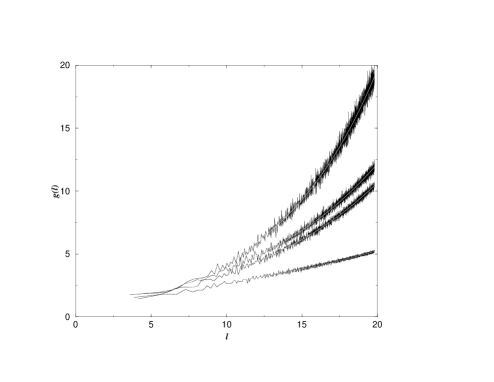
Figure 1: Mean multiplicities of periodic orbit lengths for Hecke triangles $(0,\pi/2,\pi/n)$ with (from top to bottom) $n=12$, $n=5$, $n=8$, and $n=10$ for $l<20$. White lines are numerical fits (25)–(28).

Figure 2: Mean multiplicities of periodic orbit lengths for the Hecke triangle with angles $(0,\pi/2,\pi/5)$ for $l<25$. Solid line is the fit (25).

Expressions (25)–(28) fit numerical data in the given interval of lengths pretty well. But they are purely best least-square numerical fits and no attempts were made to determine the accuracy of coefficients. In Section 5.1 it is demonstrated that our approach suggests different formulas for these quantities (see (75)) which, nevertheless, are practically indistinguishable from the above simple expressions in the considered interval of lengths (cf. Fig. 9).

For larger lengths the exponential proliferation of periodic orbits makes it difficult to compute and store in the memory all periodic orbits. Nevertheless the determination of periodic orbits in a reasonably short interval of lengths is still feasible. At Fig. 2 we present the result of the numerical computation of the length multiplicity for the Hecke triangle with $n=5$ till $l=25$. Each small circle at this figure for $l>20$ corresponds to one million of periodic orbits. The solid line is the fit (25) obtained from data at small $l$. It is clearly seen that accuracy of the fit does not change noticeably with the increasing of periodic orbit lengths.

4 Length distribution for different
isomorphisms

For the Hecke triangle groups (and for certain other groups as well) traces of group matrices are integers of an algebraic field of finite degree. Therefore each group matrix $M$ gives rise not only to one usual length (2) but to $q$ different lengths corresponded to $q$ different isomorphisms of the basis field applied to a matrix $M$. Asymptotically

$$l_{k}=2\ln|\mbox{Tr }\varphi_{k}(M)|\;.$$ (29)

In this definition $l_{1}$ corresponding to the identity transformation is the true length of a periodic orbit and all other $l_{k}$ with $k\geq 2$ are additional quantities which we call transformed lengths.

For arithmetic systems (see e.g. [4]) transformed traces are restricted

$$|\mbox{Tr }\varphi_{k}(M)|\leq 2$$ (30)

for all $k\geq 2$ which leads to the very large length multiplicities lengths for such groups (6).

The main ingredient of our approach to the problem of length multiplicity for non-arithmetic groups is the determination of the joint density of periodic orbits in intervals $l_{k},l_{k}+dl_{k}$ for all $k\geq 1$. For clarity we first consider groups with only one non-trivial isomorphisms (24) where each hyperbolic group matrix permits to define two lengths, $l_{1}$ and $l_{2}$.

Let $R(l_{1},l_{2})dl_{1}dl_{2}$ be the number of periodic orbits with the first length in the interval $l_{1},l_{1}+dl_{1}$ and the second (transformed) length in the interval $l_{2},l_{2}+dl_{2}$. Taking into account (1) one concludes that

$$R(l_{1},l_{2})\approx\frac{e^{l_{1}}}{l_{1}}P(l_{1},l_{2})$$ (31)

where $P(l_{1},l_{2})$ has the meaning of the probability density of periodic orbits with lengths $l_{1}$ and $l_{2}$ normalized such that

$$\int_{-\infty}^{\infty}P(l_{1},l_{2})dl_{2}=1\;.$$ (32)

No general arguments determining the form of $P(l_{1},l_{2})$ are known to the authors. As $l_{1}$ is only one fixed quantity with the dimension of the length, from physical considerations it is quite natural to assume that for large $l_{1}$ and $l_{2}$ this function has the following scaling form (see also Appendix B for another argument)

$$P(l_{1},l_{2})=A(l_{1})\exp\left[l_{1}f(l_{2}/l_{1})\right]$$ (33)

with a certain (smooth) scaling function $f(u)$ where $u$ is the ratio of two lengths.

When $l_{1}\to\infty$ the prefactor $A(l_{1})$ can be determined in the saddle point approximation from the normalization condition (32)

$$A(l_{1})=\frac{1}{\sqrt{2\pi\sigma^{2}l_{1}}}$$ (34)

where $\sigma^{2}=1/|f^{\prime\prime}(u_{c})|$. Here $u_{c}$ is the point of the maximum of $f(u)$: $f^{\prime}(u_{c})=0$, and $f^{\prime\prime}(u_{c})$ is the second derivative of the function $f(u)$ at this point. From (32) it follows that the value of $f(u)$ at the point of the maximum is zero

$$f(u_{c})=0\;.$$ (35)

At Fig. 3 we present numerically computed function $P(l_{1},l_{2})$ for the Hecke triangle with $n=5$ for $10^{6}$ orbits near $l_{1}\approx 19.8$ (which corresponds to $|\mbox{Tr }M|=20000$) together with the Gaussian fit to the data in the form

$$P(l_{1},l_{2})=a_{0}\exp\left(-\frac{(l_{2}-\lambda)^{2}}{2\sigma^{2}}\right)\;.$$ (36)

The least square fit gives the following values of the parameters

$$a_{0}=.116\;,\;\lambda=6.69\;,\;\sigma^{2}=11.74\;.$$ (37)

At Fig. 4 the best fit values of $\lambda(l_{1})$ and $\sigma^{2}(l_{1})$ are given for different values of $l_{1}$. The data are linear on $l_{1}$ and can be approximated by the following straight lines

$$\lambda=.330l_{1}+.187\;,\;\;\sigma^{2}=.616l_{1}-.337$$ (38)

which support the scaling ansatz (33).

The peaks at Fig. 3 correspond to words in the code (11) with a small number of letters $\alpha_{k}^{m}$ but with big values of $m$’s. Ignoring all elements except the ones multiplied by the largest possible numbers of $m$’s one can approximate the periodic orbit length as follows

$$l\approx 2\ln(\alpha^{p}\ m_{1}\ldots m_{p}\ a_{k_{1}}\ldots a_{k_{p}})\;.$$ (39)

Hence, in this approximation the difference between transformed lengths and the true length is a finite constant

$$l_{k}-l_{1}\approx 2\ln(\varphi_{k}(\alpha^{p}\ a_{k_{1}}\ldots a_{k_{p}}))-2\ln(\alpha^{p}\ a_{k_{1}}\ldots a_{k_{p}})\;.$$ (40)

To compute the joint distribution of transformed lengths one considers periodic orbits with the true length confined in a small interval. The above expression means that orbits corresponding to small numbers of initial symbols have transformed lengths at finite distances from $l_{1}$ and, consequently, they produce peaks at these distances. The quality of such approximation quickly deteriorates with increasing of $p$ due to the omitting lower powers of $m$’s and in real calculations only a few peaks with small $p$ are visible.

For the Hecke triangle with $n=5$ $a_{k}$ defined in (13) are either $1$ or $\alpha$, and all differences between two lengths are

$$l_{2}-l_{1}\approx 2m\ln\left(\frac{\sqrt{5}-1}{\sqrt{5}+1}\right)\approx-1.92\ m$$ (41)

with integer $m$ which agree well with the positions of the peaks at Fig. 3.

Figure 3: Probability density of transformed length with $l_{1}=19.8$ for the Hecke triangle with $n=5$. Thick line represents the Gaussian fit (36), (37).

Figure 4: Gaussian fit parameters (36) versus the length of periodic orbits for the Hecke triangle with $n=5$. Lower line: $\lambda$. Upper line: $\sigma^{2}$. Solid lines are the linear fits (38) to these data.

At Figs. 5-8 we plot numerically computed scaling functions $f(u)$ for the Hecke triangles with $n=5$, $n=8$, $n=10$, and $n=12$ for different intervals of periodic orbit lengths. The curves for different lengths seem to be superimposed thus supporting the scaling ansatz (33). Irregular points at $l_{2}/l_{1}\approx 1$ correspond to the above mentioned peaks (40) related with words with small number of symbols and are irrelevant at large $l_{1}$.

Figure 5: Scaling function $f(l_{2}/l_{1})$ for the Hecke triangle with $n=5$. Circles, triangles, and squares represent data for $10^{6}$ orbits near respectively $l_{1}\approx 19.8\;,\;l_{1}\approx 19.47\;,\;l_{1}\approx 19.02$. Solid line connects points with $l_{1}\approx 19.8$. Dashed line is the parabolic fit (42) to the data with $l_{1}\approx 19.8$. Thick solid line is the straight line $y=(x-1)/2$.

Figure 6: The same as at Fig. 5 but for the Hecke triangle with $n=8$.

Figure 7: The same as at Fig. 5 but for the Hecke triangle with $n=10$. Dashed line is the cubic fit (43) to the data with $l_{1}\approx 19.8$ in the interval $[.4,1]$.

Figure 8: The same as at Fig. 5 but for the Hecke triangle with $n=12$. Dashed line is the parabolic fit (44) to the data with $l_{1}\approx 19.8$ in the interval $[.1,1]$.

The scaling functions $f(l_{2}/l_{1})$ for the Hecke triangles with $n=5$ and $n=8$ are close to each other and can be reasonably well described by the following parabolic fit

$$f(x)\approx-.094+.56x-.83x^{2}$$ (42)

indicated by dashed lines at Figs. 5 and 6.

The scaling functions for the Hecke triangles with $n=10$ and $12$ have more complicated form. At Fig. 7 the dashed line indicates the cubic fit to the data in the interval $[.4,1]$

$$f(x)\approx.028-.66x+2.08x^{2}-1.77x^{3}\;.$$ (43)

At Fig. 8 the dashed line shows the parabolic fit in the interval $[.1,1]$

$$f(x)\approx-.014+.21x-.73x^{2}\;.$$ (44)

For Hecke triangle groups with $n$ different from (24) there exist more than one non-trivial isomorphisms and, consequently, the joint distribution of all lengths have the form similar to (31) but with larger number of transformed lengths

$$R(l_{1},l_{2},\ldots,l_{q})\approx\frac{e^{l_{1}}}{l_{1}}P(l_{1},l_{2},\ldots,l_{q})\;.$$ (45)

The analog of the scaling ansatz (33) in this case is

$$P(l_{1},l_{2},\ldots,l_{q})=A(l_{1})\exp\left[l_{1}f\left(\frac{l_{2}}{l_{1}},\ldots,\frac{l_{q}}{l_{1}}\right)\right]\;$$ (46)

with a certain function $f(x_{2},\ldots,x_{q})\equiv f(\vec{x})$ depended only on ratios $x_{k}=l_{k}/l_{1}$ and in the saddle point approximation

$$A(l_{1})=\sqrt{\frac{|\det\partial^{2}f/\partial x_{i}\partial x_{j}|}{(2\pi l_{1})^{q-1}}}$$ (47)

where the derivatives are taken at the point of the maximum of $f(\vec{x})$.

5 Number of periodic orbits with different lengths

The importance of the knowledge of the joint distribution of periodic orbit lengths for all possible isomorphisms is related with the fact that two periodic orbits for Hecke triangle groups have exactly the same length iff all their transformed lengths are the same.

Let us consider the simplest Hecke group with $n=5$. In this case the traces of group matrices, $t_{1}$ and $t_{2}=\varphi_{2}(t_{1})$ can be written as

$$t_{1}=n_{0}+n_{1}\lambda_{1}\;,\;\;t_{2}=n_{0}+n_{1}\lambda_{2}$$ (48)

where $n_{0},n_{1}$ are integers, $\lambda_{1}=2\cos(\pi/5)$ is an element of our basis field and $\lambda_{2}=2\cos(3\pi/5)$ is the transformed value of $\lambda_{1}$.

These equations determine the transformation from variables $t_{1},t_{2}$ to variables $n_{0},n_{1}$ and

$$dt_{1}dt_{2}=Jdn_{0}dn_{1}$$ (49)

where the Jacobian of this transformation is the square root of the discriminant (17) of the defining equation

$$J=|\lambda_{2}-\lambda_{1}|=\sqrt{\Delta_{5}}=\sqrt{5}\;.$$ (50)

As $t_{i}=e^{l_{i}/2}$ the precedent equation gives

$$dn_{0}dn_{1}=C_{5}e^{l_{1}/2+l_{2}/2}dl_{1}dl_{2}$$ (51)

with $C_{5}=1/(4\sqrt{\Delta_{5}})$.

Because $n_{0}$ and $n_{1}$ are integers this equation means that in a volume $dl_{1}dl_{2}$ there are at most $[Ce^{l_{1}/2+l_{2}/2}]$ possible values of $n_{0},n_{1}$ ($[x]$ is the integer part of x). This relation signifies that the density of the maximal number of periodic orbits with different lengths obeys asymptotically the inequality

$$\rho_{\mbox{\scriptsize diff.}}(l_{1},l_{2})\leq C_{5}e^{l_{1}/2+l_{2}/2}\;.$$ (52)

We stress that such arguments can give, in principle, the estimate from above because not all values of $n_{0}$ and $n_{1}$ are possible for the Hecke group $G_{n}$, otherwise one obtains the Hilbert modular groups which are discrete groups only in higher dimensional complex planes.

For other Hecke triangle groups with one non-trivial isomorphism (24) (i.e. for $n=8,10,12$) the defining equation is of degree 4 but traces of group matrices contain either even or odd powers of $\alpha$

$$t_{1}=n_{0}+n_{2}\alpha^{2}\;,\;\mbox{ or }\;t_{1}=n_{1}\alpha+n_{3}\alpha^{3}$$ (53)

and the result is similar to (52)

$$\rho_{\mbox{\scriptsize diff.}}(l_{1},l_{2})\leq C_{n}e^{l_{1}/2+l_{2}/2}$$ (54)

but with

$$C_{n}=\frac{1}{4\sqrt{\Delta_{n}^{(e)}}}+\frac{1}{4\sqrt{\Delta_{n}^{(o)}}}$$ (55)

where $\Delta_{n}^{(e,o)}$ are discriminants (19) and (20).

For general Hecke group with $q$ isomorphisms

$$\rho_{\mbox{\scriptsize diff.}}(l_{1},l_{2},\ldots,l_{q})\leq C_{n}e^{l_{1}/2+l_{2}/2+\ldots+l_{q}/2}\;$$ (56)

where for odd $n$

$$C_{n}=\frac{1}{2^{q}\sqrt{\Delta_{n}}}\;,$$ (57)

and for even $n$

$$C_{n}=\frac{1}{2^{q}\sqrt{\Delta_{n}^{(e)}}}+\frac{1}{2^{q}\sqrt{\Delta_{n}^{(o)}}}\;.$$ (58)

Eq. (45) means that in a volume $dl_{1}\ldots dl_{q}$ there is

$$\rho_{\mbox{\scriptsize tot.}}(\vec{l}\ )=\frac{e^{l_{1}}}{l_{1}}A(l_{1})\exp\left(l_{1}f(l_{2}/l_{1},\ldots,l_{q}/l_{1})\right)$$ (59)

periodic orbits with all transformed lengths fixed. On the other hand in the same volume the maximum number of periodic orbits with different lengths is restricted by the inequality (56)

$$\rho_{\mbox{\scriptsize diff.}}(\vec{l}\ )\leq C_{n}e^{l_{1}/2+l_{2}/2+\ldots+l_{q}/2}\;.$$ (60)

Consequently, the maximum number of periodic orbits with different lengths is

$$\rho_{\mbox{\scriptsize diff. lengths}}^{(\mbox{\scriptsize maximum})}(l_{1})=\int dl_{2}\ldots dl_{q}\left\{\begin{array}[]{cc}\rho_{\mbox{\scriptsize diff.}}(\vec{l}\ )&\mbox{ if }\;\rho_{\mbox{\scriptsize diff.}}(\vec{l}\ )\leq\rho_{\mbox{\scriptsize tot.}}(\vec{l}\ )\\ \rho_{\mbox{\scriptsize tot.}}(\vec{l}\ )&\mbox{ if }\;\rho_{\mbox{\scriptsize diff.}}(\vec{l}\ )\geq\rho_{\mbox{\scriptsize tot.}}(\vec{l}\ )\end{array}\right.\;.$$ (61)

As both densities increase exponentially with $l_{1}$ the dominant contribution to this integral is given by vicinities of boundary points where

$$\rho_{\mbox{\scriptsize diff.}}(\vec{l}\ )=\rho_{\mbox{\scriptsize tot.}}(\vec{l}\ )\;.$$ (62)

In the leading order of $l_{1}$ these points are determined from the equality of the exponential factors of these functions

$$l_{1}+l_{1}f(l_{2}/l_{1},\ldots,l_{q}/l_{1})=\frac{1}{2}(l_{1}+\ldots+l_{q})\;.$$ (63)

Denoting $l_{k}/l_{1}$ by $x_{k}$ one gets the equation independent of $l_{1}$

$$f(x_{2},\ldots,x_{q})=\frac{1}{2}(x_{2}+\ldots+x_{q}-1)\;.$$ (64)

5.1 Groups with one non-trivial isomorphism

In the simplest case of groups (24) where only one transformed length exists Eq. (64) is reduced to the equation of one variable $x\equiv x_{2}$

$$f(x)=\frac{1}{2}(x-1)\;.$$ (65)

In Appendix A it is proved that for the Hecke groups the transformed lengths corresponding to all non-trivial isomorphisms are smaller than the true length

$$l_{k}<l_{1}\;.$$ (66)

Consequently, $f(x)$ is situated at the left from the line $x=1$ and as $f(u_{c})=0$ $f(x)$ is negative when $x<1$. As $u_{c}<1$ Eq. (65) for groups with one non-trivial isomorphism always has a solution $x<1$. In Table 2 we present approximate values of this intersection point, $x_{n}$, for different values of $n$ found from Figs. 5–8.

Table 2: Parameters for Hecke triangles with $n=5\;,\;8\;,\;10\;,\;12$. The second column is the curvature in the point of the maximum. The third column gives the value of $C_{n}$ in (54). The fourth and the fifth columns are the ordinate of the intersection point and the modulus of the slope of $f(x)$ at this point. The nest three columns are parameters in (74). The last column gives the numerically computed prefactor in (75).

$n$	$\sigma_{n}^{2}$	$C_{n}$	$x_{n}$	$k_{n}$	$\lambda_{n}$	$\nu_{n}$	$G_{n}$	$K_{n}$
$5$	$.6$	$.11$	$.74$	$.66$	$.13$	$.35$	$1.32$	$2.34$
$8$	$.6$	$.15$	$.74$	$.66$	$.13$	$.35$	$1.11$	$2.22$
$10$	$.55$	$.16$	$.82$	$.82$	$.09$	$.43$	$1.22$	$2.46$
$12$	$.68$	$.14$	$.64$	$.73$	$.18$	$.39$	$1.25$	$1.77$

As claimed in all these cases the solution exists and $x_{n}<1$.

In the next order one can write

$$l_{2}=x_{n}l_{1}+\varepsilon_{n}\;.$$ (67)

Expanding Eq. (62) to the first order of $\varepsilon$ one gets

$$C_{n}\sqrt{2\pi\sigma_{n}^{2}l_{1}^{3}}=\exp(-\varepsilon_{n}(k_{n}+.5)+{\cal O}(\varepsilon_{n}^{2}/l_{1}))$$ (68)

where $k_{n}=|f^{\prime}(x_{n})|$ is the modulus of the derivatives at the point of the intersection. Therefore

$$\varepsilon_{n}=-\frac{1}{k_{n}+.5}\ln\left(C_{n}\sqrt{2\pi\sigma_{n}^{2}}l_{1}^{3/2}\right)\;.$$ (69)

Together these formulas demonstrate that for the Hecke triangles (24) at the intersection point

$$\rho_{\mbox{\scriptsize diff.}}(l_{1},l_{2})=\rho_{\mbox{\scriptsize tot.}}(l_{1},l_{2})\approx D_{n}e^{l_{1}(1+x_{n})/2}l_{1}^{-3\beta_{n}/2}$$ (70)

where

$$\beta_{n}=\frac{1}{2k_{n}+1}\;,\;\;D_{n}=\frac{C_{n}^{1-\beta_{n}}}{(2\pi\sigma_{n})^{\beta_{n}/2}}\;.$$ (71)

The integration in (61) in the limit of large $l_{1}$ can be performed by parts and finally

$$\rho_{\mbox{\scriptsize diff. lengths}}^{(\mbox{\scriptsize maximum})}(l_{1})=\frac{2D_{n}}{1-\beta_{n}}\frac{e^{l_{1}(1+x_{n})/2}}{l_{1}^{3\beta_{n}/2}}\;.$$ (72)

The mean multiplicity of periodic orbit lengths is the ratio of the total density of periodic orbits to the density of orbits with different lengths. Hence

$$\bar{g}(l)\geq G_{n}\frac{e^{\lambda_{n}l}}{l^{\nu_{n}}}$$ (73)

where

$$\lambda_{n}=\frac{1-x_{n}}{2}\;,\;\;\nu_{n}=1-\frac{3}{2}\beta_{n}\;,\;\;G_{n}=\frac{1-\beta_{n}}{2D_{n}}\;.$$ (74)

At Table 2 we present approximate values of these parameters computed from Figs. 5–8. At Fig. 9 we compare data of length multiplicities for the Hecke triangles (25)–(28) with the formula of the form (73)

$$\bar{g}(l)=K_{n}\frac{e^{\lambda_{n}l}}{l^{\nu_{n}}}$$ (75)

with the computed values of $\lambda_{n}$ and $\nu_{n}$ from Table 2 but with a prefactor $K_{n}$ calculated from the best fit to the data (see the last column of Table 2). The ‘theoretical’ curves (75) are practically indistinguishable from the best fits (25)–(28). Note that fitted prefactors is always bigger than $G_{n}$, just confirming that estimates (73) and (74) give only lower bounds. Though in principle not all integers are allowed in (21), these results seem to indicate that in the mean the ratio of the density of allowed integers to all integers for the groups (24) is finite.

Figure 9: Comparison of numerically computed fits (25)–(28) for length multiplicities for Hecke triangles (dotted lines) with formulas (75) with fitted prefactor (solid lines). From top to bottom: $n=12$, $n=5$, $n=8$, $n=10$.

5.2 General case

For general case of $q>2$ isomorphisms the arguments, in principle, remain the same. One has to perform the following three steps:

• to check that required solutions of Eq. (64) do exist,

• to find on $(q-2)$-dimensional manifold of these solutions a point with the maximum of the sum $x_{2}+\ldots+x_{q}$,

• to compute the integral (61) in a small vicinity of the point of the maximum.

For groups with only one non-trivial isomorphism the inequality (66) was sufficient to ensure the existence of a solution of Eq. (64). For other groups it is not the case and one has to rely mostly on numerical calculations. For example, the necessary condition of the existence of solutions of Eq. (64) is that at the point $u_{2},\ldots,u_{q}$ of the maximum of the scaling function $f(x_{2},\ldots,x_{q})$ the sum $u_{2}+\ldots+u_{q}$ is less than $1$.

At Fig. 10 we present the contour plot of the scaling function $f(x_{2},x_{3})$ for the Hecke triangle group with $n=7$ computed from $10^{6}$ points near $l_{1}=25$. The contour lines correspond to the sections of the scaling function (normalized so that at the maximum it equals zero) at heights $-2\cdot 10^{-4}k(2k-1)$ for $k=1,\ldots,9$.

Figure 10: Contour plot of the scaling function $f(l_{2}/l_{1},l_{3}/l_{1})$ for the Hecke triangle with $n=7$. Thick line is the solution of equation $f(x_{2},x_{3})=(x_{2}+x_{3}-1)/2$.

Numerically from this figure one gets that for the Hecke group with $n=7$ the solution of equation $f(x_{2},x_{3})=(x_{2}+x_{3}-1)/2$ do exist and the point with the maximum $x_{2}+x_{3}$ corresponds approximately to the fourth contour line. It means that the density of maximal number of different periodic orbit lengths increases as

$$\rho_{\mbox{\scriptsize diff. lengths}}^{(\mbox{\scriptsize maximum})}(l_{1})\sim e^{(1-\lambda_{7})l_{1}}$$ (76)

where $\lambda_{7}\approx.006$. Correspondingly, the mean multiplicity of periodic orbit lengths can be estimated (without a prefactor) as

$$\bar{g}(l_{1})>e^{.006l_{1}}\;.$$ (77)

Though it is an exponential increase, the exponent is so small that at really accessible lengths $l_{1}$ of the order of $20$ it practically remains a constant and the prefactor dominates. At Fig. 11 we plot the numerically computed mean multiplicity for the Hecke triangle group with $n=7$ (averaged over interval of traces equal 10). Instead of increasing it shows a slow decrease but the best fit to the data in the form

$$\bar{g}=a\frac{e^{bl}}{l^{c}}$$ (78)

gives

$$a\approx 3.55\;,\;\;b\approx.007\;,\;\;c\approx.168\;$$ (79)

which is larger than (77). Unfortunately, the limited interval of lengths and very slow increase of the multiplicity do not permit to obtain clear conclusions.

At Fig. 12 numerically computed length multiplicities for the Hecke triangles with $n=9$ and $n=11$ are presented. Similarly to the $n=7$ case the data indicate a slow decrease which is more pronounced for the $n=11$ triangle. Is this decrease just a lower-length phenomenon or do multiplicities in these cases tend to a constant cannot be answered from the accessible data.

We stress that though the data for the Hecke triangles with $n=7$, $n=9$, and $n=11$ do not show clear increase of mean multiplicities they fluctuate around values bigger than $2$ which differs from the usual expectation. Also in all figures we present multiplicities averaged over some length. The true multiplicities fluctuate wildly around the mean confirming unusual character of the Hecke triangle groups.

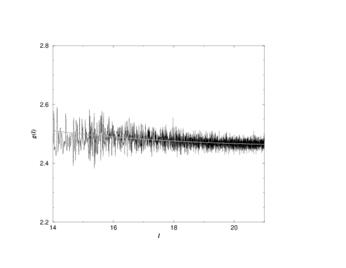
Figure 11: Mean multiplicity for the Hecke triangle with $n=7$. Solid line is the fit (78), (79).

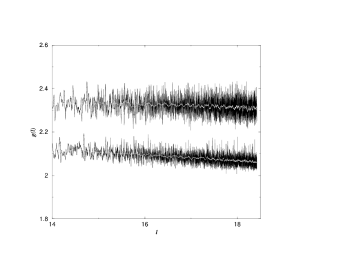
Figure 12: Mean multiplicities for the Hecke triangles with $n=9$ (the upper curve) and $n=11$ (the lower curve). White lines represent additional smoothing of the curves.

6 Spectral statistics of non-arithmetic Hecke triangles

It is well accepted that length degeneracy of periodic orbits has a profound effect on spectral statistics. According to semiclassical theory of spectral statistics [1], [2] the two-point correlation form factor for chaotic billiards in the diagonal approximation is

$$K^{(\mbox{\scriptsize diag.})}(t)=\bar{g}(l(t))t$$ (80)

where $\bar{g}(l)$ is the mean multiplicity of periodic orbits with the length $l$ and $l(t)=4\pi kt$.

For systems without (resp. with) time-reversal invariance $\bar{g}=1$ (resp. $\bar{g}=2$) and (80) gives the first term of the expansion of the two-point correlation form factors for standard random matrix ensembles (see e.g. [3]).

For models considered in the preceding Sections the mean multiplicity $\bar{g}(l)$ increases exponentially as in (75) and the form factor calculated in the diagonal approximation differs from the random matrix predictions.

To consider the spectral statistics we compute numerically eigenvalues of the Laplace-Beltrami operator with the Dirichlet conditions on the boundaries of the Hecke triangles for different values of $n$. At Fig. 13 we present the differences between the integrated nearest-neighbor distributions and the Wigner ansatz for this quantity ($N_{W}(s)=1-e^{\pi s^{2}/4}$) for the Hecke triangles with $n=5,\;7,\;12$. For comparison on these graphs thick solid lines indicate the difference between the true GOE formula and the Wigner ansatz. From the figure it is clearly seen that spectral statistics for the Hecke triangles is quite close to the conjectured statistics of the Gaussian Orthogonal Ensemble (GOE) of random matrices.

Figure 13: Differences between integrated nearest-neighbor distributions for the Hecke triangles and the Wigner ansatz for this quantity (thick solid lines). Top - the first 10000 levels for the triangle with $n=5$, middle - the first 20000 for the triangle with $n=7$, bottom - the first 10000 levels for the triangle with $n=12$. Dashded line - the same quantities but for the triangles with angles $10\pi/119$, $10\pi/71$, $20\pi/99$, respectively. Thick solid lines at each graph are the difference between the true GOE prediction and the Wigner ansatz.

To have an estimate of statistical errors we compute numerically the same quantities (dashed lines at Fig. 13) for non-tesselating triangles of the Hecke type which have two angles $\pi/2$ and $0$ but instead of the angle $\pi/n$ as for the true Hecke triangle we take a certain angle $\gamma_{n}$ sufficiently close to it. For $n=5,\;7,\;12$ we choose respectively

$$\gamma_{5}=\frac{20\pi}{99}\;,\;\gamma_{7}=\frac{10\pi}{71}\;,\;\gamma_{12}=\frac{10\pi}{119}\;.$$ (81)

Notice that the difference between $\gamma_{n}$ and $\pi/n$ is quite small

$$\left|\gamma_{5}-\frac{\pi}{5}\right|\approx 6\cdot 10^{-3}\;,\;\left|\gamma_{7}-\frac{\pi}{7}\right|\approx 6\cdot 10^{-3}\;,\;\left|\gamma_{12}-\frac{\pi}{12}\right|\approx 2\cdot 10^{-3}\;.$$ (82)

For all cases (except possible small deviations for $n=12$ which has the largest multiplicities) the nearest-neighbor distributions for the Hecke triangles agree well with the curves for non-tesselating triangles

These (and others) figures demonstrate that the spectral statistics of the non-arithmetic Hecke triangles (even with quite large degeneracies of periodic orbit lengths) at small distances is rather well described by standard random matrix ensembles.

The contradiction between the observed random matrix statistics of the Hecke triangles and deviations of correlation functions due to large multiplicities of periodic orbits (cf. (80) was partially resolved in [4]. In this paper it was demonstrated that the diagonal approximation can, strictly speaking, be applied only for very small values of $t<t_{1}$. If the mean multiplicity increases like $\bar{g}(l)\sim e^{\lambda l}$ with a certain constant $\lambda\leq 1/2$ from [4] it follows that the time of applicability of the diagonal approximation has the following estimate

$$t_{1}\sim\frac{1}{1-\lambda}\frac{\ln k}{k}\;.$$ (83)

During this time the form factor increases exponentially but it can reach only a value of the order of

$$K(t_{1})\sim k^{-(1-2\lambda)/(1-\lambda)}\;.$$ (84)

For arithmetic systems $\lambda=1/2$ (see [4]) and the form factor for the time of applicability of the diagonal approximation becomes of the order of $1$ which explains the Poisson character of their spectral statistics. But for all non-arithmetic groups $\lambda$ is less than $1/2$ and the form factor in the diagonal approximation increases only by a negative power of $k$. Therefore in the semiclassical limit $k\to\infty$ there is no apparent contradiction between observed $GOE$-type local statistics and the change of correlation functions due to large multiplicities of periodic orbits.

These arguments suggest that two-point form factors for non-arithmetic Hecke triangles has the form indicated at Fig. 14. The peak at small values of $t$ is due to large multiplicities of periodic orbits. The magnitude of this peak and its position seem to decrease for large $k$.

Figure 14: Schematic form of the two-point correlation form factor for non-arithmetic Hecke triangles. Dashed line is the continuation of the GOE form factor to small values of $t$.

Though deviations from standard statistics should be small when $k\to\infty$ the peak indicated at Fig. 14 may influence the large distance spectral properties like the number variance (see e.g. [3]). At Fig. 15-17 we present the number variance for the Hecke triangles with $n=5,\;7,\;12$ together with the corresponding values for non-tesselating triangles (81). Due to large statistical errors in the computation of the number variance $\Sigma^{2}(L)$ we found convenient to plot at the figures not $\Sigma^{2}(L)$ itself but its averaged value defined in the following way

$$<\Sigma^{2}(L)>\equiv\frac{1}{L}\int_{0}^{L}\Sigma^{2}(l)dl\;.$$ (85)

To demonstrate the evolution of the number variance with increasing the energy at all figures we present pictures for the averaged number variance with different number of levels.

Figure 15: Smoothed number variance for the Hecke triangle with $n=5$ (top graphs). Different type of lines corresponds to the number variance computed from the first $2000\cdot k$ levels. Solid line - $k=1$, dotted line - $k=2$, dashed line - $k=3$, long dashed line - $k=4$, dot-dashed line - $k=5$. Thick line is the GOE prediction. Bottom graphs represent the same quantities for the non-tesselating triangle with angle $\gamma_{5}=20\pi/99$. For clarity top graphs are shifted up by .2 unit.

Figure 16: The same as at Fig. 15 but for the Hecke triable with $n=7$ (top graphs). Different types of lines correspond to the averaged number variance computed from the first $4000\cdot k$ levels. Bottom graphs are calculated for the non-tesselating triangle with angle $\gamma_{7}=10\pi/71$.

Figure 17: The same as at Fig. 15 but for the Hecke triangle with $n=12$ (top graphs). Bottom graphs are calculated for the non-tesselating triangle with angle $\gamma_{12}=10\pi/119$.

For all non-tesselating (generic) triangles the number variance follows the the GOE prediction for small values of $L$ and then saturates, as it should be for dynamical systems [1], [2]. For the Hecke triangles the number variance at small $L$ also agrees with the GOE formula but then it becomes bigger than this reference expression and only later it saturates but at a value different from the one of the corresponding very close-by non-tesselating triangle.

This overshooting looks as a direct confirmation of the conjectured form of the two-point correlation form factor (cf. Fig. 14) but careful calculation of this quantity requires a ressumation of, at least certain, non-diagonal terms and is beyond the scope of this paper.

7 Summary

We demonstrate both numerically and analytically that, at least, certain non-arithmetic Hecke triangle groups have exponentially large multiplicities of periodic orbit lengths.

In groups under consideration matrix elements of group matrices are integers of an algebraic field of a finite degree and each group matrix gives rise naturally to $q$ different lengths corresponding to $q$ different isomorphisms of the basis field. The main ingredient of our approach to the problem of periodic orbit length multiplicity is the investigation of the joint distribution of periodic orbits with all $q$ transformed lengths fixed.

We conjecture that this distribution has a scaling form (46) and find the scaling exponent numerically. For Hecke groups (24) with only one non-trivial isomorphism the general inequality (66) is sufficient to demonstrate an exponential increase of the multiplicities. Multiplicities obtained by this method are in a good agreement with direct numerical calculations.

For general Hecke triangle groups we are not aware of analytical conditions of the existence of necessary solutions. In all investigated cases (except for the groups (24) with only one non-trivial isomorphism) the increase of multiplicities numerically is too small to be observed from direct calculations of periodic orbits but the data fluctuate around a value bigger than $2$.

The spectral statistics of non-arithmetic Hecke triangles agrees with the GOE statistics at small distances but deviates from usual expectations at large distances.

Acknowledgments

The authors are very grateful to T. Schmidt for pointing out Refs. [15] and [7], and to O. Bohigas for useful discussions.

Appendix A

To prove the inequality (66) it is slightly more convenient to describe conjugacy classes of the Hecke triangle group matrices not by the code discussed in Section 2 but by a code proposed in [16] better suitable for analytical calculations. In this code the letters for the orientation preserving subgroup of $G_{n}$ are the following matrices

$$g_{k}(\alpha_{n})=U^{k-1}T\;,\;\;\;k=1,\ldots,n-1\;,$$ (86)

where $U=TS$ and matrices $T$, $S$ are the translation and inversion matrices which generate the whole group $G_{n}$

$$T=\left(\begin{array}[]{cc}1&\alpha\\ 0&1\end{array}\right)\;,\;\;S=\left(\begin{array}[]{cc}0&-1\\ 1&0\end{array}\right)$$ (87)

with $\alpha=2\cos\pi/n$.

As in the previous code periodic orbits for the Hecke group $G_{n}$ (with unit determinant) are free words of letters $g_{k}$, the only restriction being that all cyclic permutations of a word give one orbit.

It is easy to check (e.g. by induction) that

$$g_{k}=\left(\begin{array}[]{cc}a_{k}&a_{k+1}\\ a_{k-1}&a_{k}\end{array}\right)$$ (88)

where $a_{k}\equiv a_{k}(2\cos\theta)$ are the values of the Chebyshev polynomials of the second kind

$$a_{k}(2\cos\theta)=\frac{\sin(k\theta)}{\sin\theta}\;.$$ (89)

computed at $\theta=\pi/n$.

Let us introduce the following definition. We say that a function $f(x)$ has the H-property with a separating point $h$ if

$$|f(x)|\leq f(h)\;\mbox{ for all }\;|x|\leq h\;.$$ (90)

The importance of this notion follows from the fact that if $f_{1}(x)$ and $f_{2}(x)$ both have the H-property with separating point $h$ then $f_{1}(x)f_{2}(x)$ and $f_{1}(x)+f_{2}(x)$ also have the H-property with the same separating point. In particular, if one has a set of matrices whose elements all have the H-property with a separating point $h$ then all products of these matrices also have the H-property with the same separating point.

Let us prove first that matrix elements $a_{k}$ with $k=0,\ldots,n$ have the H-property with the separating point $h=2\cos(\pi/2n)$. Indeed

$$\left|a_{k}(2\cos\theta)\right|\leq\frac{1}{\sin\theta}\;.$$ (91)

When $0\leq\theta\leq\pi/2$ the equality sign in this inequality holds at the points

$$\theta_{m}=\frac{\pi}{2k}m$$ (92)

where $m$ is an odd integer $1\leq m\leq k$.

Therefore when $\theta\geq\pi/2k$

$$\left|a_{k}(2\cos\theta)\right|\leq\frac{1}{\sin\theta}\leq a_{k}(2\cos\frac{\pi}{2k})\;.$$ (93)

Moreover, $a_{k}(2\cos\theta)$ is a decreasing function when $0<\theta<\pi/2k$ and $a_{k}(2\cos\theta)\leq a_{k}(2\cos\pi/2n)$ when $\pi/2n\leq\theta\leq\pi/2k$ (and, of course, $k\leq n$). Together these two inequalities prove that $a_{k}$ with $k\leq n$ have the H-property with separating point $h=2\cos(\pi/2n)$.

Second, $a_{k}(2\cos\pi p/n)=a_{n-k}(2\cos\pi p/n)$ for odd integer $p$. It means that for all isomorphisms (22) $a_{k}(x)$ equals $a_{n-k}(x)$ and only $a_{k}$ with $k\leq n/2$ are independent. Hence, $a_{k}$ for all isomorphisms of the defining equation can be considered as polynomials of degree not greater than $n/2$ and one can choose for all $a_{k}(2\cos\pi p/n)$ with $k\leq n$ the same separating constant $h=2\cos(\pi/n)$.

Third, as was stated above, all matrix elements obtained by taking the products of arbitrary number of matrices $g_{k}$ also have the H-property with the separating constant $h=2\cos(\pi/n)$.

Combining all these arguments one proves that for all isomorphisms of the basis field traces of the Hecke group matrices have the H-property with the same separating constant. Because

$$\left|\cos\frac{\pi k}{n}\right|<\cos\frac{\pi}{n}$$ (94)

for all $k\neq 0,1,n$ one gets that modulus of traces of the Hecke triangle group matrices decrease for all non-trivial isomorphisms of the basis field thus proving the inequality (66). For matrices with determinant equal $-1$ the same inequality follows by computing the square of such matrices because the periodic orbit length for the square of any matrix is twice the length corresponding to the initial matrix.

After this paper has been completed we become aware of Ref. [15] where the inequality (66) was proved for all groups which permit the so-called modular embedding. From Ref. [7] it follows that all triangle discrete groups belong to this class. Therefore, the inequality (66) is valid for all triangle groups (and not only for the Hecke triangle groups considered in this paper).

Appendix B

The purpose of this Appendix is to give arguments in favor of the representation (33) of the joint probability density of periodic orbits with all transformed lengths fixed.

For discrete groups periodic orbits can be obtained from product of certain number of matrices. Let us consider in a given code the product of $n$ basis matrices

$$A(n)=A_{n}\cdot A_{n-1}\cdots A_{1}\;.$$ (95)

The total number of matrices with $n$ symbols for a general code is exponential

$$\rho(n)\stackrel{{\scriptstyle n\to\infty}}{{\longrightarrow}}\frac{e^{hn}}{n}$$ (96)

where $h$ is a constant called the topological entropy.

The length of periodic orbit is related with matrix $A$ asymptotically as

$$l=2\ln\mbox{ Tr }A\;.$$ (97)

Therefore, matrices representing periodic orbits can be considered as the result of a random process where matrices $A_{k}$ are chosen randomly from a code grammar. The probability distribution of lengths for products of $n$ such matrices is defined as the ratio of number of matrices with lengths in the interval $[l,l+dl]$ divided by total number of matrices.

This distribution under quite general conditions [8], [10] has the Gaussian form

$$P_{n}(l)=\frac{1}{\sqrt{2\pi}\sigma_{n}}e^{-\frac{(l-l_{n})^{2}}{2\sigma_{n}^{2}}}$$ (98)

where

$$l_{n}=\lambda_{0}n\;,\;\;\;\sigma_{n}^{2}=\sigma_{0}^{2}n\;.$$ (99)

One of possible applications of such distribution is the calculation of the total density of periodic orbits of length $l$ (see e.g. [14])

$$\rho(l)=\int\frac{e^{hn}}{n}P_{n}(l)dn\;.$$ (100)

When $l\to\infty$ the integral can be computed in the saddle point approximation and the total density of periodic orbits has exponential asymptotics

$$\rho(l)=\frac{e^{\kappa l}}{l}$$ (101)

where

$$\kappa=\frac{\lambda_{0}-\sqrt{\lambda_{0}^{2}-2h\sigma_{0}^{2}}}{\sigma_{0}^{2}}\;.$$ (102)

For groups considered in the paper all matrix elements belong to an algebraic field of a finite degree which has $q$ different isomorphisms. It means, in particular, that each product of $n$ group matrices $A(n)$ as in (95) gives rise to $q$ different lengths $l_{i}(n)$ obtained by applying each isomorphism $\varphi_{i}$ to $A(n)$

$$l_{i}(n)=2\ln|\mbox{Tr}\varphi_{i}(A(n))|\;.$$ (103)

On the other hand $\varphi_{i}(A(n))$ can be obtained as the product of $n$ transformed matrices $\varphi_{i}(A_{k})$ as in (95). Therefore according to the above theorem each variable $l_{i}$ is a random variable whose distribution also has asymptotically the Gaussian form

$$P_{n}(l_{i})=\frac{1}{\sqrt{2\pi n}\sigma_{i}}e^{-\frac{(l_{i}-\lambda_{i}n)^{2}}{2n\sigma_{i}^{2}}}$$ (104)

with certain parameters $\lambda_{i}$ and $\sigma_{i}$ having the meaning of the mean value and the variance of $l_{i}(n)$.

Let us conjectured that the mutual distribution of all $l_{i}(n)$ together is also Gaussian

$$P_{n}(\vec{l}\ )=\frac{\sqrt{\det M}}{(2\pi)^{q/2}}\exp\left(-\frac{1}{2n}\sum_{ij=1}^{q}M_{ij}(l_{i}-\lambda_{i}n)(l_{j}-\lambda_{j}n)\right)$$ (105)

with a certain positive definite matrix $M_{ij}$.

Analogously to Eq. (100) the total density of orbits with fixed $l_{i}$ is

$$\rho(\vec{l}\ )=\int_{1}^{\infty}\frac{e^{hn}}{n}P_{n}(\vec{l}\ )dn\;.$$ (106)

As above this integral can be computed in the saddle point approximation valid at large $\vec{l}$ and the result is

$$\rho(\vec{l}\ )=\frac{\sqrt{\det M}}{(2\pi)^{(q-1)/2}(A(C-2h))^{1/4}}\exp\left(B-\sqrt{A(C-2h)}\right)$$ (107)

where

$$A=\sum_{i,j=1}^{q}M_{ij}l_{i}l_{j}\;,\;\;B=\sum_{i,j=1}^{q}M_{ij}l_{i}\lambda_{j}\;,\;\;C=\sum_{i,j=1}^{q}M_{ij}\lambda_{i}\lambda_{j}\;.$$ (108)

The exponent in (107) is an homogeneous function of $l_{j}$ and after the rescaling $x_{j}=l_{j}/l_{1}$ one obtains the scaling ansatz (46) with a specific scaling function which leads to exponential asymptotics of the joint probability distribution as it seems suggested by numerics (cf. Figs. 5-8).

The main drawback of such approach is that the theorem about the Gaussian form of the distribution of the product of $n$ random matrices is valid only near the maximum of the distribution. But the term $e^{hn}$ in (100) and (107) shifts the saddle point far from the maximum and there exist no general arguments which would imply the smallness of corrections to the parabolic form of the exponent. For certain groups and special codes it seems that one can ignore such corrections in a region of interest but, in general, corrections are large and one has to rely on the numerics as it was done in the main part of the paper.

References

- [1] M. Berry, Semiclassical theory of spectral rigidity, Proc. R. Soc. Lond. A 400 (1985) 229.
- [2] M. Berry, Some quantum-to-classical asymptotics, in [9], (1991) 250-303.
- [3] O. Bohigas, Random matrix theories and chaotic dynamics, in [9], (1991) 86-199.
- [4] E. Bogomolny, B. Georgeot, M.-J. Giannoni, and C. Schmit, Arithmetical Chaos, Phys. Rep. 291 (1997) 219-326.
- [5] E. Bogomolny, E. Leyvraz, and C. Schmit, Distribution of eigenvalues for the modular group, Commun. Math. Phys. 176 (1996) 577.
- [6] J. Bolte, G. Steil, and F. Steiner, Arithmetical chaos and violations of universality in energy level statistics, Phys. Rev. Lett. 69 (1992) 43.
- [7] P. Cohen and J. Wolfart, Modular embeddings for some non-arithmetic Fuchsian groups, Acta Arith. 61 (1990) 93-110.
- [8] H. Furstenberg, Non-commuting Random Products, Trans. Amer. Math. Soc. 108 (1963) 377-428.
- [9] Chaos and Quantum Physics, Proceeding of the Les Houches summer school (1989), Eds. M.-J. Giannoni, A. Voros, J. Zinn-Justin, North Holand, Amsterdam, London, New York, Tokyo (1991).
- [10] I. Ya. Goldsheid and Y. Guivach, Zariski Closure and the Dimension of the Gaussian Law for Products of Random Matrices . I., Prob. Theory and Related Fields, 105 (1996) 109-142.
- [11] D.A. Hejhal, The Selberg trace formula and the Riemann zeta function, Duke Math. J. 43 (1976) 441.
- [12] R.D. Horowitz, Characters of free groups represented in the two-dimensional special linear group, Commun. Pure Appl. Math. 25 (1972) 635.
- [13] E. Randol, The length spectrum of Riemann surface is always of unbounded multiplicity, Proc. Amer. Math. Soc. 78 (1980) 455.
- [14] M. Sieber, The hyperbola billiard: a model for semiclassical quantization of chaotic systems, PhD thesis, Hamburg (1991).
- [15] P. S. Schaller and J. Wolfart, Semi-arithmetic Fuchsian groups and modular embeddings, J. London Math. Soc. 61 (2000) 13-24.
- [16] T.A. Schmidt and M. Sheingorn, Length spectra of the Hecke triangle group, Math. Z. 220 (1995) 369-397.