Synchronization of globally coupled nonidentical maps with inhomogeneous delayed interactions

Abstract

We study the synchronization of a coupled map lattice consisting of a one-dimensional chain of logistic maps. We consider global coupling with a time-delay that takes into account the finite velocity of propagation of interactions. We recently showed that clustering occurs for weak coupling, while for strong coupling the array synchronizes into a global state where each element sees all other elements in its current, present state [Physica A 325 (2003) 186, Phys. Rev. E 67 (2003) 056219]. In this paper we study the effects of in-homogeneities, both in the individual maps, which are non-identical maps evolving in period-2 orbits, and in the connection links, which have non-uniform strengths. We find that the global synchronization regime occurring for strong coupling is robust to heterogeneities: for strong enough average coupling the inhomogeneous array still synchronizes in a global state in which each element sees the other elements in positions close to its current state. However, the clustering behaviour occurring for small coupling is sensitive to inhomogeneities and differs from that occurring in the homogeneous array.

,

Globally coupled units with time delays and inhomogeneous interactions arise in a variety of fields. In the fields of economics and social sciences, a multi-agent model that allows for temporally distributed asymmetric interactions between agents was recently proposed in Ref. [1]. The model defined a coupled map lattice with interactions obeying a Gaussian law and transmitted through a gamma pattern of delays. In the field of optics, a globally coupled laser array with feedback has been proposed for exploring the complex dynamics of systems with high connectivity [2, 3, 4]. Globally and locally coupled maps have been employed to study synchronization [5] in a great variety of fields ranging from activity patterns in pulse-coupled neuron ensembles [6, 7] to dynamics models of atmospheric circulation [8].

Since they were introduced by Kaneko, globally coupled logistic maps have turned out to be a paradigmatic example in the study of spatiotemporal dynamics in extended chaotic systems [9]. In the simplest form all maps are identical and interact via their mean field with a common coupling:

$$x_{i}(t+1)=(1-\varepsilon)f[x_{i}(t)]+{{\varepsilon}\over{N}}\sum_{j=1}^{N}f[x_{j}(t)].$$ (1)

Here $t$ is a discrete time index, $i$ is a discrete spatial index: $i=1\dots N$ where $N$ is the system size, $f(x)=ax(1-x)$ is the logistic map, and $\varepsilon$ is the coupling strength. Even though the model has only two parameters (the common nonlinearity $a$ and the coupling strength $\varepsilon$), it exhibits a rich variety of behaviours. For a large $\epsilon$ the maps synchronize in a global state, and evolve together as a single logistic map. For intermediate coupling the array divides into two clusters ($x_{i}(t)=x_{j}(t)$ if $i$ and $j$ belong to the same cluster) which oscillate in opposite phases. For small coupling the number of clusters increases but is nearly independent of the total number of maps in the system. Finally, for very small coupling the number of clusters is proportional to $N$ [10].

We have recently studied effect of time-delayed interactions [11, 12]. We considered the array:

$$x_{i}(t+1)=(1-\varepsilon)f[x_{i}(t)]+{{\varepsilon}\over{N}}\sum_{j=1}^{N}f[x_{j}(t-\tau_{ij})]$$ (2)

where $\tau_{ij}$ is a time delay, proportional to the distance between the $i$th and $j$th maps. We took $\tau_{ij}=k|i-j|$, where $k$ is the inverse of the velocity of the interaction signal traveling along the array.

We found that for weak coupling the array divides into clusters, and the behavior of the individual maps within each cluster depends on the delay times. For strong enough coupling, the array synchronizes into a single cluster (globally synchronized state). In this state the elements of the array evolve along a orbit of the uncoupled map, while the spatial correlation along the array is such that an individual map sees all other maps in his present, current, state:

$$x_{j}(t-\tau_{ij})=x_{i}(t).$$ (3)

It was also found that for values of the nonlinear parameter $a$ such that the uncoupled maps are chaotic, time-delayed mutual coupling suppress the chaotic behavior by stabilizing a periodic orbit which is unstable for the uncoupled maps.

In this paper we extend the previous study to assess the influence of heterogeneities. We consider the following array:

$$x_{i}(t+1)=(1-\varepsilon_{i})f[a_{i},x_{i}(t)]+{{1}\over{N}}\sum_{j=1}^{N}\varepsilon_{i,j}f[a_{j},x_{j}(t-\tau_{ij})]$$ (4)

where $f(a,x)=ax(1-x)$, $\varepsilon_{i,j}$ is the strength of the link coupling the maps $i$ and $j$, $\varepsilon_{i}$ is the average connection strength of the site $i$:

$$\varepsilon_{i}={{1}\over{N}}\sum_{j=1}^{N}\varepsilon_{i,j}$$ (5)

and $\tau_{ij}=k|i-j|$. We perform numerical simulations with the aim of studying the effects of inhomogeneities in the maps and in the strength of the coupling links. We consider two different situations:

1) Nonidentical maps coupled with identical coupling strengths ($\epsilon_{i,j}=\epsilon$ $\forall$ $i$, $j$). The value of $a_{i}$ is random, uniformly distributed in the interval ($a_{0}-\delta a$,$a_{0}+\delta a$). We limit ourselves to consider maps in the period-2 region ($a_{i}\in[3,3.449\dots]$). The study of the synchronization of the array when the individual maps without coupling are either in fixed points or in period-$n$ orbits is left for future work.

2) Identical maps ($a_{i}=a_{0}$ $\forall$ $i$) coupled with nonindentical links. In this case we consider two different situations: (a) The value of $\varepsilon_{i,j}$ random, uniformly distributed in the interval (0,$\epsilon$). (b) $\varepsilon_{i,j}$ varies in interval [0,$\epsilon$], such that the strength of a link decreases with its length. We take $\varepsilon_{i,j}=\epsilon[1-\tau_{i,j}/\max(\tau_{i,j})]$. It can be noticed from Eqs. (4,5) that the globally synchronized state Eq.(3) is also an exact solution of the array when the maps are identical but the connection strengths are not.

Let us first illustrate the transition to global synchronization in the case of inhomogeneous maps connected through homogeneous links ($\epsilon_{i,j}=\epsilon$ $\forall$ $i$,$j$). We exemplify results for $k$ odd. For $k$ odd the globally synchronized state of the homogeneous array is the anti-phase state: $x^{A}_{i}(t)=x_{a},x_{b},x_{a},\dots$; $x^{A}_{i}(t+1)=x_{b},x_{a},x_{b},\dots$. Here $x_{a}$ and $x_{b}$ are the points of the limit cycle of the map $f(a_{0},x)$. Similar results are observed for $k$ even (in this case the globally synchronized state is the in-phase state: $x^{I}_{i}(t)=x_{a},x_{a},x_{a},\dots$; $x^{I}_{i}(t+1)=x_{b},x_{b},x_{b},\dots$).

Figures 1(a) and 1(b) display bifurcation diagrams for increasing $\epsilon$, which were done in the following way: we chose a random initial condition [$x_{i}(0)$ with $i=1,\dots,N$], and plotted a certain number of time-consecutive values of $x_{i}(t)$ (with $t$ large enough and $i=1,\dots,N$) vs. the coupling strength $\epsilon$. Since the initial condition fixes the cluster partition of the array, the same initial condition was used for all values of $\epsilon$. For comparison, Fig. 1(a) displays the bifurcation diagram for a homogeneous chain ($\delta a=0$), while Fig. 1(b) displays results for $\delta a=0.2$. While a sharp transition to global synchronization is observed for $\delta a=0$, a smoother transition, reminiscent of bifurcations in the presence of noise, is observed for $\delta a\not=0$. To illustrate this transition with more detail we show in Fig. 2 the configuration of the array for several values of $\epsilon$ (the values of $\epsilon$ are indicated with an arrow in Fig. 1). It is observed that the array gradually evolves to the antiphase state. For low $\epsilon$ there is a large dispersion in the values of $x_{i}$ and defects are observed. The dispersion and the number of defects gradually diminishes as $\epsilon$ increases.

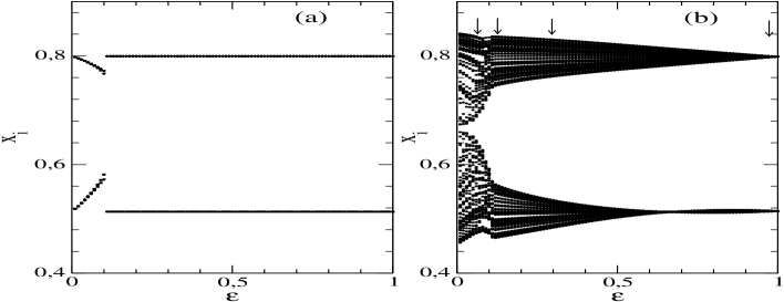
Figure 1: Bifurcation diagram for homogeneous (a) ($\delta a=0.$) and inhomogeneous (b) ($\delta a=0.2$) array. Parameter values: $a=3.2$, $k=1$, and $N=100$.

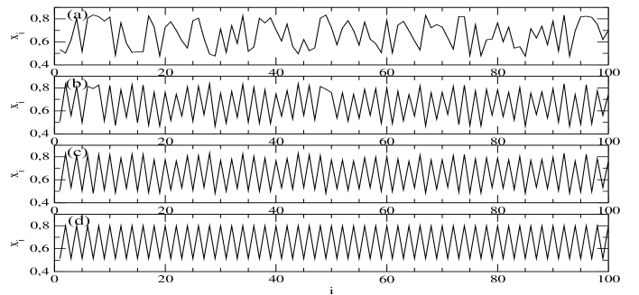
Figure 2: Array configuration at time $t=3000$, for different values of the coupling strength $\epsilon$ (a) $\epsilon=0.07$, (b) $\epsilon=0.11$, (c) $\epsilon=0.29$, and (d) $\epsilon=0.98$ . Other parameters as in Fig. 1 .

Next we study the case of homogeneous maps ($a_{i}=a_{0}$ $\forall$ $i$) connected through inhomogeneous links. Figure 3 displays bifurcation diagrams done in the same way as in Fig. 1, i.e., taking the same initial configuration of the array for all values of $\epsilon$. However, in this case the links have different coupling strengths [$\varepsilon_{i,j}$ varies in (0,$\varepsilon$), is either uniformly distributed or decreasing with $\tau_{i,j}$]. Therefore, in the horizontal axis we plotted the average coupling strength $<\varepsilon>=1/N^{2}\sum_{i}\sum_{j}\varepsilon_{i,j}$. It can be observed that as $<\varepsilon>$ increases there is a sharp transition to global synchronization, both when $\epsilon_{i,j}$ is randomly distributed in (0,$\epsilon$), and when $\epsilon_{i,j}$ is in (0,$\epsilon$) decreasing with distance. However, there is different clustering behaviour, as illustrated in Fig. 4. Figures 4(a) and (b) display the clustering behaviour for $k=1$ (we point out that for $k=1$ and $<\varepsilon>$ large enough the array synchronizes in anti-phase), and Figs. 4(c) and (d) display the clustering behaviour for $k=2$ (for $k=2$ and $<\varepsilon>$ large enough the array synchronizes in-phase). For comparison, Figs. 4(a) and 4(c) display the clustering behaviour of the homogeneous array. In these figures $\epsilon_{i,j}=\epsilon_{0}$ with $\epsilon_{0}$ equal to the average coupling strength in Figs. 4(b) and 4(d). In spite of the fact that the average connection strength is the same, the partition of the array is different when the connection links have non-uniform strengths.

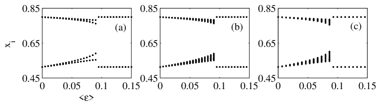
Figure 3: Bifurcation diagram displaying the transition to the globally synchronized state. $N=100$, $a_{i}=3.2$ $\forall$ $i$, and $k=1$. (a) $\varepsilon_{i,j}=\varepsilon_{0}$ $\forall$ $i$ and $j$; (b) $\varepsilon_{i,j}$ is uniformly distributed in $(0,\epsilon$); (c) $\varepsilon_{i,j}$ decreases with distance.

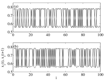
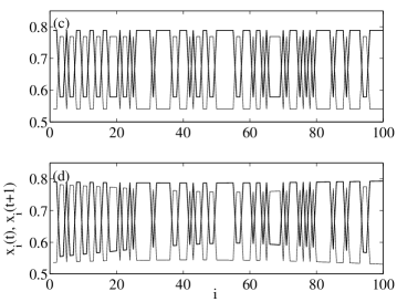
Figure 4: Clustering behaviour for weak coupling strength. The thin line shows the array configuration at time $t$, and the thick line shows the array configuration at time $t+1$. $N=100$ and $a_{i}=3.2$ $\forall$ $i$. (a) $k=1$ and $\varepsilon_{i,j}=0.08$ $\forall$ $i$,$j$; (b) $k=1$ and $\varepsilon_{i,j}$ uniformly distributed in [0,0.16], $<\varepsilon_{i,j}>=0.08$; (c) $k=2$ and $\varepsilon_{i,j}=0.073$ $\forall$ $i$,$j$; (d) $k=2$ and $\epsilon_{i,j}\in(0,0.11)$ decreases with distance, $<\varepsilon_{i,j}>=0.073$.

To quantify the effect of in-homogeneities we introduce the following quantity

$$\sigma(t)=\sqrt{{{1}\over{N}}\sum_{i}[x_{i}(t)-x^{R}_{i}(t)]^{2}},$$ (6)

that measures the deviation of the array configuration, $x_{i}(t)$, from a given reference state, $x^{R}_{i}(t)$. $x_{i}(t)$ is evaluated at time $t$ with $t$ long enough to let transients die away. The reference state is the anti-phase state for $k$ odd ($x^{R}_{i}(t)=x_{a},x_{b},x_{a},\dots$; $x^{R}_{i}(t+1)=x_{b},x_{a},x_{b},\dots$) and the in-phase state for $k$ even ($x^{R}_{i}(t)=x_{a},x_{a},x_{a},\dots$; $x^{R}_{i}(t+1)=x_{b},x_{b},x_{b},\dots$). Here $x_{a}$ and $x_{b}$ the points of the limit cycle of the map $f(a_{0},x)$.

Figure 5 shows $<\sigma>$ vs. $\epsilon$ where $<\cdot>$ represents an average over different initial configurations $x_{i}(0)$. We observe here that in the homogeneous array (solid line) the decay of the deviation $\sigma$ is more abrupt that in the heterogeneous array (dashed line). This is due to related to the sharp transition to global synchronization shown in Fig. 1.

To summarize, we have studied the effect of the inhomogeneities in a linear chain of globally coupled logistic maps with time-delayled interactions. The inhomogeneities occurs both in the individual maps which are non-identical and in the connection link which have non-uniform strengths. We considered the case in which the maps, without coupling, evolve in a limit cycle of period $P=2$. We found that the global synchronization regime occurring for strong coupling is robust to heterogeneities: for strong enough average coupling the inhomogeneous array still synchronizes in a global state in which each element sees the other elements in positions close to its current state. However, the clustering behaviour occurring for small coupling is sensitive to inhomogeneities and differs from that occurring in the homogeneous array.

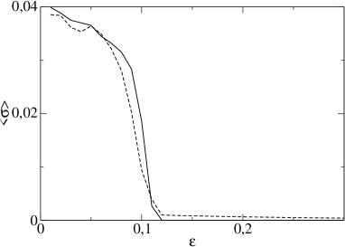
Figure 5: Deviation of the array configuration vs coupling strength averaged over 100 realizations for the cases with (continuous line, $\delta a=0.2$) and without dispersion (dashed line, $\delta a=0$). (Parameter values: $N=100$, $k=1$, $a=3.2$)

References

- [1] C. J. Emmanouilides, S. Kasderidis, and J. G. Taylor, Physica D 181 (2003) 102-120.
- [2] K. Otsuka and J-L Chern, Phys. Rev. A 45 (1992) 5052-5055.
- [3] J. García-Ojalvo, J. Casademont, C. R. Mirasso, M. C. Torrent, and J. M. Sancho, Int. J. Bifurcation Chaos 9 (1999) 2225-2229.
- [4] G. Kozyreff, A. G. Vladimirov, and Paul Mandel, Phys. Rev. Lett. 85 (2000) 3809-3812.
- [5] A.S. Pikovsky, M.G. Rosenblum, and J. Kurths, Synchronization-A Universal Concept in Nonlinear Sciences, Cambridge University Press, Cambridge, 2001.
- [6] G. V. Osipov and J. Kurths, Phys. Rev. E 65 (2001) 016216.
- [7] H. Haken, Brain Dynamics: Synchronization and activity patterns in pulse-coupled neural nets with delays and noise, Springer Series in Synergetics.
- [8] P.G. Lind, João Corte-Real and Jason A.C. Gallas, Physical Review E, 66 (2002) 016219.
- [9] K. Kaneko, Phys. Rev. Lett. 63 (1989) 219.
- [10] T. Shimada and K. Kikuchi, Phys. Rev. E 62 (2000) 3489-3503.
- [11] C. Masoller, A. C. Marti and D. H. Zanette, Physica A 325 (2003) 186-191.
- [12] A. C. Marti and C. Masoller, Phys. Rev. E 67 (2003) 056219-1-6.