Instabilities induced by a weak breaking of a strong spatial resonance

Abstract

Through multiple-scales and symmetry arguments we derive a model set of amplitude equations describing the interaction of two steady-state pattern-forming instabilities, in the case that the wavelengths of the instabilities are nearly in the ratio $1:2$. In the case of exact $1:2$ resonance the amplitude equations are ODEs; here they are PDEs.

We discuss the stability of spatially-periodic solutions to long-wavelength disturbances. By including these modulational effects we are able to explore the relevance of the exact $1:2$ results to spatially-extended physical systems for parameter values near to this codimension-two bifurcation point. These new instabilities can be described in terms of reduced ‘normal form’ PDEs near various secondary codimension-two points. The robust heteroclinic cycle in the ODEs is destabilised by long-wavelength perturbations and a stable periodic orbit is generated that lies close to the cycle. An analytic expression giving the approximate period of this orbit is derived.

, , and

1 Introduction

Pattern-forming instabilities occur in many physical problems, for example Rayleigh-Bénard convection, Faraday wave experiments and directional solidification [8]. In some of these situations well-established governing equations are available which are sufficiently simple to analyse. In others the situation is not so clear cut, and reductions to model equations are of great value. The derivation of model equations to describe instabilities in these physical problems often provides a clear and unified viewpoint, bringing out similarities in the underlying mathematical structure.

In one spatially-extended dimension, the study of the stability of spatially-periodic patterns that arise from a steady-state bifurcation with continuous translational symmetry often reduces to the investigation of an evolution equation, for example the Ginzburg–Landau equation. Such equations, derived by asymptotic methods rather than rigorous analysis (though see recent work by Melbourne [17]) can both comprehend uniform spatially-periodic patterns and describe their stability to long-wavelength disturbances.

In the present paper we consider the case when two distinct instability mechanisms are present, for example in two-layer thermal convection [23]. Here the two instabilities will typically have different preferred horizontal lengthscales given by the critical wavenumbers corresponding to local minima in the curves of marginal stability. Each instability separately can be described by a ‘universal’ model equation such as the Ginzburg–Landau equation. However, the two instability mechanisms interact nonlinearly if the instabilities occur for similar values of the control parameters; this is a codimension-2 bifurcation. In such a situation more complicated model equations are needed to describe the dynamics in the region of parameter space near the codimension-2 point. The form of these model equations will depend on the symmetry of the problem, the steady or oscillatory nature of the instabilities, and on the ratio of the critical wavenumbers.

When the critical wavenumber ratio is rational (say $p/q$ where $p$ and $q$ are coprime integers) we may restrict attention to solutions which are periodic in the horizontal direction and derive, in a mathematically rigorous fashion using a centre manifold reduction, ODEs describing the dynamics on the centre manifold at the point of instability. The cases $p=1$, $q=1,2,3$ have been termed ‘strong’ spatial resonances since the nonlinear interaction terms generated appear at third order, or below, in the resulting amplitude equations.

When the ratio is irrational this centre-manifold approach cannot be applied. Any restriction to spatially-periodic solutions will not be able to capture important features of the dynamics. In consequence the periodic solutions found may be unstable to long-wavelength instabilities, and their subsequent evolution must be described by PDEs rather than ODEs. In this case, there is currently no rigorous mathematical formulation which leads to PDEs. At best the equations used represent asymptotic approximations to the true situation. Nonetheless we shall adopt the PDE approach here, following the work of (among others) Coullet & Repaux [5], since it is natural and has proved very productive in similar, though simpler, problems.

In this paper we discuss the interaction of two steady-state instabilities with wavenumbers close to, but not exactly in, the ratio $1:2$, using multiple-scales expansions in time and space. The case of exact $1:2$ resonance was treated first by Dangelmayr [9] and later by Jones & Proctor [13] and by Proctor & Jones [23] (hereafter referred to as Part 1) in the context of two-layer thermal convection. Important results were also obtained by Armbruster et al. [1] and Julien [12], and more recently by Porter & Knobloch [20]. In particular, [12] resolved several contradictions and errors in the earlier papers mentioned above, and investigated the dynamics of the ODEs away from the codimension-2 point; a full description of the dynamics of the ODEs becomes very involved. Here we extend this work and show that small deviations from the exact $1:2$ situation result in additional long-wavelength instabilities of otherwise stable spatially periodic patterns (‘spatial quasiperiodicity’).

The most unusual part of the dynamics of the $1:2$ resonance problem is the occurrence of a structurally stable heteroclinic cycle. The local information that we are able compute near the equilibria on the cycle enables analysis of the stability of the cycle to long-wavelength spatial disturbances.

The equations that we derive to capture these modulational instabilities are nonlinear PDEs, and as such, a full analysis is a daunting task. Indeed, even a complete classification of possible solutions is far beyond the scope of this paper. This paper considers those parts of the problem that can be treated analytically rather than presenting a superabundance of numerical results. Our analysis explores the stability of spatially-periodic equilibria and travelling waves, identifying those new instabilities that are due to the inclusion of modulational effects. The dynamics near these new instabilities can be described by ‘normal form’ equations (simpler PDEs whose structure is often prescribed by symmetry requirements). Although the algebraic expressions may become lengthy, it is possible to reduce the original nonlinear PDEs to these ‘normal forms’ explicitly via adiabatic elimination. Such a reduction, although not completely rigorously justified, can be extremely useful, particularly near secondary codimension-2 points (intersections of lines of codimension-1 bifurcations away from the initial bifurcation point). The paper illustrates this idea with two explicit detailed examples (the points $\mathbb{L}$ and $\mathbb{X}$ in figure 1); in neither case is the ‘normal form’ equation the Ginzburg–Landau equation. The dynamics near $\mathbb{L}$ have been well-studied in the literature, but those near $\mathbb{X}$ are more novel.

The original study of Part 1 was motivated by a particular two-layer thermal convection problem, and we refer the interested reader to that paper for detailed discussion of the physical background. Wavenumber interactions in the ratio $1:2$ also occur in two-dimensional thermal convection in a single layer, for example in the asymptotic long-wavelength equation discussed by Cox [7], and in non-Boussinesq convection as discussed by Mercader, Prat & Knobloch [18, 21]. These papers discuss situations that have one instability mechanism; by looking for solutions that are spatially-periodic with a given wavenumber $k$ they locate codimension-two points $(R_{c},k_{c})$ where two periodic patterns interact, with wavenumbers in the ratio $1:2$. Since, in these problems, $R_{c}$ is always greater than the minimum value required to drive convection in a formally infinite layer, the results are not directly applicable to the infinite layer case. In contrast, this paper (formally) attempts to analyse the infinite-layer situation in the case where there are two distinct instability mechanisms occurring for very similar values of the control parameters. The large horizontal extent of the layer enables periodic patterns to be destabilised by ‘sideband’ instabilities, for example the Eckhaus instability. We remark that a similar study, for ‘weak’ resonances, has been performed recently by Higuera, Riecke & Silber [11]. Their results, although very different in detail, have points of similarity to those presented here, for example the existence of solutions in the form of localised structures.

The paper is organised as follows. In section 2 we derive the model equations and make general remarks about the dynamics. In section 3 we briefly summarise the dynamics of the model ODEs in the absence of the modulational terms. Here and throughout the rest of the paper we use a single combination of coefficients that were used in Part 1, for ease of comparison. Sections 4 and 5 discuss in detail the new instabilities of spatially-periodic states that occur when the modulational terms are added to the model. In section 6 we discuss the stability of the robust heteroclinic cycle. Analytic work shows the existence of a long-period periodic orbit lying close to the cycle, in quantitative agreement with numerical results. Section 7 briefly highlights the coexistence, over a substantial region of the parameter plane, of stable non-modulated travelling waves and complex spatiotemporal behaviour. We conclude in section 8.

2 Model equations near $1:2$ resonance

Consider a horizontal two-dimensional layer, or layers, of fluid in the domain $(-\infty,\infty)\times[0,1]$, using co-ordinates $(x,z)$, i.e. of finite vertical extent but extending to infinity in the horizontal direction $x$. We suppose that there is an $x$-independent state which may become linearly unstable to either of two competing steady-state instabilities, with wavenumbers nearly in the ratio $1:2$. By way of illustration, the analysis of Part 1 was concerned with a two-layer thermal convection problem where these two instabilities corresponded to the onset of convection predominantly in either the upper or the lower layer separately. The most interesting dynamics can be captured by the distinguished limit in which the deviation of the ratio of the critical wavenumbers from the exact value $\frac{1}{2}$ is of the order of the square root of the deviation of the bifurcation parameter (in this case the Rayleigh number $R$) from its critical value $R_{c}$. If we set $R-R_{c}=\varepsilon^{2}$ then we may write the critical wavenumbers (those associated with local minima in the value of the critical Rayleigh number) as $k+\varepsilon q$ and $2k$. A suitable ansatz for small-amplitude solutions near the codimension-2 point where the conditions for instability coincide is then

$$u(x,z,t) = \varepsilon\left[A(X,T)f_{1}(z)\mathrm{e}^{\mathrm{i}x(1+\varepsilon q)}+B(X,T)f_{2}(z)\mathrm{e}^{2\mathrm{i}x}+c.c.\right]$$ (1)

$$+O(\varepsilon^{2}),$$

where lengths have been rescaled so that $k=1$; $X=\varepsilon x$ and $T=\varepsilon^{2}t$ are long length and time scales, $c.c.$ denotes complex conjugate, and the functions $f_{1,2}(z)$ give the vertical structure of the eigenfunction corresponding to each mode of instability. The amplitudes $A(X,T)$, $B(X,T)$ are complex-valued. The initial homogeneous state is symmetric under the Euclidean group $E(1)$ generated by the reflection $m_{x}:x\rightarrow-x$ and the translations $\tau_{\delta}:x\rightarrow x+\delta$. These symmetries induce the following transformations on the amplitudes $A$ and $B$:

$$m_{x}: x\rightarrow-x: \qquad(A,B)\rightarrow(\bar{A},\bar{B}),$$ (2)

$$\tau_{\delta}: \ \ x\rightarrow x+\delta: \qquad(A,B)\rightarrow(A\mathrm{e}^{\mathrm{i}(1+\varepsilon q)\delta},B\mathrm{e}^{2\mathrm{i}\delta}).$$ (3)

The combination $\bar{A}^{2}B\mathrm{e}^{2\mathrm{i}qX}$ is found to be the lowest-order translation-invariant combination that is not a product of the usual terms $|A|^{2}$ and $|B|^{2}$.

The resulting amplitude equations (ignoring terms of order higher than three in $A$, $B$ and $\partial_{X}$) take the form

$$\dot{A} = A[\mu_{1}-a_{1}|A|^{2}-b_{1}|B|^{2}]+a_{3}\bar{A}B\mathrm{e}^{2\mathrm{i}qX}+a_{4}A_{XX},$$ (4)

$$\dot{B} = B[\mu_{2}-a_{2}|B|^{2}-b_{2}|A|^{2}]+b_{3}A^{2}\mathrm{e}^{-2\mathrm{i}qX}+cB_{XX},$$ (5)

where the coefficients $a_{j}$, $b_{j}$ and $c$ are forced to be real by the reflection symmetry (2), the dots denote derivatives with respect to the slow time scale $T$ and $\mu_{1}$, $\mu_{2}$ are bifurcation parameters. We remark that (4) - (5) contain both quadratic and cubic terms in the amplitudes $A$ and $B$. To ensure a rational scheme of approximation in the limit $\varepsilon\rightarrow 0$ we should arrange that $a_{3},b_{3}$ scale as $\varepsilon$. This can be achieved in several ways, for example where a further symmetry which would leave the equations invariant under the sign change $(A,B)\rightarrow(-A,-B)$ is weakly broken.

The form of equations (4) - (5) shows that when $|q|$ becomes large the spatially-averaged contribution from the quadratic terms decreases to zero. In this limit we formally recover the usual ‘Landau’ equations describing two coupled modes of instability in the absence of spatial resonance. This is in agreement with our ansatz (1); the system is far from the $1:2$ mode interaction point when $|q|\sim O(1/\varepsilon)$.

Subsequent calculations are made considerably easier if we make the change of variable $\hat{A}=A\mathrm{e}^{-\mathrm{i}qX}$ to remove the exponential factors, and rescale the variables $A$, $B$, $T$ and $X$ to set $a_{3}=a_{4}=1$ and $b_{3}=\pm 1$. Dropping the carat on $\hat{A}$ we obtain

$$\dot{A} = A[\mu_{1}-q^{2}-a_{1}|A|^{2}-b_{1}|B|^{2}]+\bar{A}B+2\mathrm{i}qA_{X}+A_{XX},$$ (6)

$$\dot{B} = B[\mu_{2}-a_{2}|B|^{2}-b_{2}|A|^{2}]\pm A^{2}+cB_{XX},$$ (7)

which is the form of the equations that we will use in what follows. These equations have the same structure as the ODEs derived in Part 1 with the addition of terms giving modulation on the long lengthscale $X$. The term $2\mathrm{i}qA_{X}$ captures the effect of the departure from exact $1:2$ resonance.

Writing $A=R(X,T)\mathrm{e}^{\mathrm{i}\theta(X,T)}$ and $B=S(X,T)\mathrm{e}^{\mathrm{i}\phi(X,T)}$, the evolution equations (6) - (7) become

$$\dot{R} = R[\mu_{1}-q^{2}-a_{1}R^{2}-b_{1}S^{2}]+RS\cos\raise 2.0pt\hbox{$\chi$}-2qR\theta_{X}+R_{XX}-R(\theta_{X})^{2},$$ (8)

$$R\dot{\theta} = RS\sin\raise 2.0pt\hbox{$\chi$}+2qR_{X}+2R_{X}\theta_{X}+R\theta_{XX},$$ (9)

$$\dot{S} = S[\mu_{2}-a_{2}S^{2}-b_{2}R^{2}]\pm R^{2}\cos\raise 2.0pt\hbox{$\chi$}+c[S_{XX}-S(\phi_{X})^{2}],$$ (10)

$$S\dot{\phi} = \mp R^{2}\sin\raise 2.0pt\hbox{$\chi$}+c[2S_{X}\phi_{X}+S\phi_{XX}],$$ (11)

where $\raise 2.0pt\hbox{$\chi$}\equiv\phi-2\theta$. When the modulational terms are omitted, we can express the dynamics in terms of only the two moduli and the one phase difference $\chi$ (i.e. a reduction to a third-order system), as was done in Part 1. This leads to the ODEs

$$\dot{R} = R[\mu_{1}-q^{2}-a_{1}R^{2}-b_{1}S^{2}]+RS\cos\raise 2.0pt\hbox{$\chi$},$$ (12)

$$\dot{S} = S[\mu_{2}-a_{2}S^{2}-b_{2}R^{2}]\pm R^{2}\cos\raise 2.0pt\hbox{$\chi$},$$ (13)

$$\dot{\raise 2.0pt\hbox{$\chi$}} = \left(\mp\frac{R^{2}}{S}-2S\right)\sin\raise 2.0pt\hbox{$\chi$}.$$ (14)

However, in the presence of modulational terms, each of the individual phase variables $\theta$ and $\phi$ is dynamically independent. Vyshkind & Rabinovich [24] introduced the new variables $u=S\cos\raise 2.0pt\hbox{$\chi$}$, $v=S\sin\raise 2.0pt\hbox{$\chi$}$ (also used by Porter & Knobloch [20]) to produce a third-order system avoiding the co-ordinate singularity, but this change of variables offers no simplification in the PDE problem.

The choice of the sign of the $\pm A^{2}$ term in (7) has a huge effect on the dynamics. It was shown in Part 1 that in the ‘$+$’ case for the non-modulated problem the dynamics are much less interesting than those may occur in the ‘$-$’ case. Indeed in the ‘$+$’ case there is a Lyapounov functional $V(R,\theta,S,\phi)$ for the dynamics when $2b_{1}=b_{2}$:

$$V=\left<\frac{a_{1}}{2}R^{4}\right. + \frac{a_{2}}{4}S^{4}+b_{1}R^{2}S^{2}-\frac{\mu_{2}}{2}S^{2}-\mu_{1}R^{2}+R_{X}^{2}+R^{2}(\theta_{X}+q)^{2}$$

$$- R^{2}\left.S\cos\raise 2.0pt\hbox{$\chi$}+\frac{c}{2}[S_{X}^{2}+S^{2}\phi_{X}^{2}]\right>,$$

where $\left<\cdots\right>$ denotes a horizontal average. Then a direct calculation shows that

$$\dot{V}=-\left<2\dot{R}^{2}+2R^{2}\dot{\theta}^{2}+\dot{S}^{2}+S^{2}\dot{\phi}^{2}\right>\leq 0,$$

i.e. the system evolves monotonically towards a steady state. More complicated dynamics, for example temporal oscillations, are not possible. It follows that, at least when $2b_{1}$ and $b_{2}$ are not widely different, or the amplitudes are small (equivalently, near to the codimension-2 point), we expect solution trajectories to tend asymptotically to equilibria after long times.

For the remainder of the paper we consider the ‘$-$’ case, choosing the minus sign in (7). In this case it is not possible to construct a Lyapounov functional, and even in the absence of modulational terms the related ODE problem (12) - (14) can indeed display oscillatory dynamics; moreover there is a region of parameter space where a robust heteroclinic cycle exists and is stable. This cycle was analysed in Part 1 and by Armbruster et al. [1]. The parameter $c$ in (7) corresponds to differential diffusion rates of the two amplitudes. Varying $c$ away from unity leads to Turing instabilities, well-known in the context of reaction-diffusion equations. We remove this complicating consideration by setting $c=1$ in nearly all of what follows. The occurrence of Turing instabilities in mode interactions is common to all cases of strong spatial resonance and is of a different type to the instabilities we discuss here, since it occurs in the spatially-extended but exactly-resonance case. A full discussion of this second class of instabilities is given in a companion paper ([22], in preparation).

3 Non-modulational dynamics near $\mu_{1}=\mu_{2}=0$

In this section we summarise the relevant parts of the bifurcation sequences observed in Part 1 near $\mu_{1}=\mu_{2}=0$ in the analysis of the ODEs (12) - (14), setting $q=0$. As remarked on earlier, even in the absence of the modulational terms, a full analysis of (6) - (7) is extremely complicated.

The trivial equilibrium $A=B=0$ is stable in the quadrant $\mu_{1}<0$, $\mu_{2}<0$. Near the codimension-2 point at $\mu_{1}=\mu_{2}=0$, the ODEs (12) - (14) support simple non-trivial equilibrium solutions of three types. The first type is a pure mode solution $P$, of the form $A=0$, $|B|^{2}=\mu_{2}/a_{2}$. The continuous symmetry of the problem implies the existence of a group orbit of equilibria; that is, the phase of $B$ is arbitrary due to the underlying translational symmetry. Within the subspace $\mathrm{Fix}(m_{x})$ where $A,B\in\mathbb{R}$ there are two equilibria, denoted $P_{\pm}$. The pure mode solutions bifurcate from the trivial solution and exist when $\mu_{2}>0$. They are stable for $\mu_{1}$ sufficiently negative. The other equilibria are mixed mode equilibria of two kinds, $M_{\pm}$, corresponding to $\chi$ taking the values $\raise 2.0pt\hbox{$\chi$}=0$ and $\raise 2.0pt\hbox{$\chi$}=\pi$, respectively. The $M_{\pm}$ amplitudes $R=R_{0}$ and $S=S_{0}$ are given by solutions of the equations

$$0 = \mu_{1}\pm S_{0}-a_{1}R_{0}^{2}-b_{1}S_{0}^{2},$$ (16)

$$0 = \mu_{2}S_{0}\mp R_{0}^{2}-a_{2}S_{0}^{3}-b_{2}R_{0}^{2}S_{0}.$$ (17)

where the sign choices select either $M_{+}$ or $M_{-}$. In fact there is a group orbit of each of $M_{+}$ and $M_{-}$ equilibria also, since although $\chi$ is fixed at $0$ or $\pi$ respectively, there is a free choice of one of the underlying phases $\theta$ or $\phi$. When $\mu_{1}$ is increased, holding $\mu_{2}>0$ fixed, stable $M_{+}$ equilibria are created in a bifurcation at which the pure mode solutions lose stability.

The $M_{+}$ solution then loses stability (as $\mu_{1}$ is increased further) either through a symmetry-breaking drift bifurcation which produces travelling waves (TW), or through a Hopf bifurcation to standing waves (SW). The TW solution resembles the mixed-mode $M_{+}$ in form, but it drifts along the group orbit of mixed-mode solutions as time evolves. The TW bifurcation is clearly a phase instability rather than an amplitude instability. Because the phase variables $\theta$ and $\phi$ evolve at constant rates such that $\chi$ is constant and $\sin\raise 2.0pt\hbox{$\chi$}\neq 0$, the TW solutions appear as equilibria in the $(R,S,\raise 2.0pt\hbox{$\chi$})$ variables. In other words, the use of the $(R,S,\raise 2.0pt\hbox{$\chi$})$ variables identifies all points on the group orbit of $M_{+}$ solutions as a single equilibrium, and, in these co-ordinates, information about drift around group orbits is lost.

In contrast, the SW bifurcation is an amplitude-driven instability and produces periodic orbits that lie within the subspace $\raise 2.0pt\hbox{$\chi$}=0$. Typical curves along which $M_{+}$ undergoes bifurcations to TW or SW solutions are shown in figure 1. For a large region of parameter space these two curves intersect at a codimension-2 point, labelled $\mathbb{A}$ in figure 1. Because the eigenvectors corresponding to the TW and SW bifurcations are orthogonal the codimension-two bifurcation corresponding to simultaneous instability is a pitchfork–Hopf bifurcation (in the $(R,S,\raise 2.0pt\hbox{$\chi$})$ co-ordinates).

(a) (b)

Figure 1: (a) Instability boundaries in the $(\mu_{1},\mu_{2})$ plane for the illustrative coefficient choices $a_{1}=1$, $a_{2}=5$, $b_{1}=2$, $b_{2}=0$, $c=1$, $q=0.2$. Unstable and stable solutions in each region are indicated with and without parentheses. The solid curve containing the point $\mathbb{L}$ denotes the boundary of existence of $M_{+}$. The solid curves $TW$ and $SW$ denote instabilities of $M_{+}$ to travelling and standing waves respectively. The codimension-2 points $\mathbb{A}$, $\mathbb{X}$, $\mathbb{Y}$, $\mathbb{L}$, $\mathbb{S}$ and $\mathbb{T}$ and the various dashed and dash-dotted curves are discussed in the text. (b) is an enlargement of (a).

As we increase $\mu_{1}$ for small positive $\mu_{2}$, the SW instability occurs first. Within the subspace $\mathrm{Fix}(m_{x})$ the periodic orbit created in the SW bifurcation grows until it collides simultaneously with the origin and the $P_{+}$ equilibrium. After this global bifurcation the periodic orbit disappears, but now the unstable manifold of $P_{+}$ tends asymptotically to the pure mode solution $P_{-}$. By symmetry, within the invariant subspace $\mathrm{Fix}(m_{x}\circ\tau_{\pi})$ the unstable manifold of $P_{-}$ tends to $P_{+}$, and a heteroclinic cycle is formed. The heteroclinic cycle is structurally stable due to the existence of invariant subspaces, within which each connecting trajectory lies. Hence it exists for an open set of values of the coefficients and bifurcation parameters. Moreover, this cycle is attracting for an open interval of values of $\mu_{1}$.

At larger $\mu_{1}$ this cycle ceases to attract nearby trajectories as it undergoes a resonant bifurcation, resulting in a global loss of stability, and creating modulated waves (MW). MW are destroyed in a Hopf bifurcation from the TW which themselves cease to exist in a bifurcation with the $M_{-}$ states. Moreover, several other heteroclinic cycles are possible for other combinations of coefficients, and at larger positive $\mu_{2}$. These have been investigated in detail by Porter & Knobloch [20].

4 Modulational instability of the pure mode

Having summarised the behaviour of the system in the absence of spatial modulations, we now allow $q$ to take non-zero values, and examine the possibility of new modes of instability due to the spatial frequency mismatch. We first note that the results of Part 1, summarised in the previous section, apply within the subspace of non-modulated ($X$-independent) solutions. To examine the stability of the pure mode solution $P_{+}$, given by $A=0$ and $B=B_{0}\equiv\sqrt{\mu_{2}/a_{2}}$, we substitute the ansatz

$$A(X,T) = \alpha_{1}(T)\mathrm{e}^{\mathrm{i}\ell X}+\bar{\alpha}_{2}(T)\mathrm{e}^{-\mathrm{i}\ell X},$$

$$B(X,T) = B_{0}(1+\beta_{1}(T)\mathrm{e}^{\mathrm{i}mX}+\bar{\beta}_{2}(T)\mathrm{e}^{-\mathrm{i}mX}),$$

into (6) - (7) and linearise. The linearised dynamics for $\alpha_{1,2}$ and $\beta_{1,2}$ decouple and $P_{+}$ is found to be stable to the perturbations $\beta_{1,2}$ for all wavenumbers $m$. The linearised system for the perturbations $\alpha_{1,2}$ is

$$\left(\begin{array}[]{c}\dot{\alpha}_{1}\\ \dot{\alpha}_{2}\end{array}\right) = \left(\begin{array}[]{cc}\mu_{1}-q^{2}-b_{1}B_{0}^{2}-2q\ell-\ell^{2}&B_{0}\\ B_{0}&\mu_{1}-q^{2}-b_{1}B_{0}^{2}+2q\ell-\ell^{2}\end{array}\right)\left(\begin{array}[]{c}\alpha_{1}\\ \alpha_{2}\end{array}\right).$$ (24)

This matrix has trace $\mathrm{tr}(\ell^{2})$ and determinant $D(\ell^{2})$:

$$\mathrm{tr}(\ell^{2}) = 2(\mu_{1}-q^{2}-\ell^{2}-b_{1}B_{0}^{2}),$$

$$D(\ell^{2}) = (\mu_{1}-q^{2}-\ell^{2}-b_{1}B_{0}^{2})^{2}-4q^{2}\ell^{2}-B_{0}^{2}.$$

No oscillatory bifurcation is possible since $\mathrm{tr}(\ell^{2})=0$ implies $D(\ell^{2})<0$. A steady-state instability to perturbations with wavenumber $\ell$ occurs when $D(\ell^{2})=D^{\prime}(\ell^{2})=0$ since $D^{\prime\prime}(\ell^{2})=2>0$. These conditions show that the first instability of $P_{+}$ may be to perturbations either with $\ell=0$ or with $\ell$ non-zero. When $\mu_{2}>a_{2}(\mu_{1}+q^{2})/b_{1}$ the first instability is to $\ell=0$ and occurs along the curve $\mu_{1}=b_{1}\mu_{2}/a_{2}+q^{2}-\sqrt{\mu_{2}/a_{2}}$. When $\mu_{2}<a_{2}(\mu_{1}+q^{2})/b_{1}$ the first instability is to finite $\ell=\ell_{c}>0$ and occurs along the line

$$\mu_{1} = \frac{\mu_{2}}{a_{2}}\left(b_{1}-\frac{1}{4q^{2}}\right).$$

These two instability curves meet at the point $(\mu_{1}^{\mathbb{L}},\mu_{2}^{\mathbb{L}})=(4b_{1}q^{4}-q^{2},4a_{2}q^{4})$, marked $\mathbb{L}$ on figure 1. The gradients of these curves are equal here, so the transition between instabilities is smooth. Along the line $\mathbb{O}\mathbb{L}$ (from the origin to $\mathbb{L}$) the most unstable wavenumber, $\ell_{c}$, is given by $\ell_{c}^{2}=\mu_{1}-b_{1}\mu_{2}/a_{2}+q^{2}$, i.e. $0<\ell_{c}<q$, and $\ell_{c}$ increases monotonically as the origin is approached.

At any point on the interior of the line $\mathbb{O}\mathbb{L}$ we can fully describe this bifurcation by the usual Ginzburg–Landau equation, since for the PDEs (6) - (7) this is an instability of a uniform state to a nonzero-wavelength perturbation, and the growth rate of a perturbation with a wavenumber far from $\ell_{c}$ is negative and bounded away from zero. We have carried out a weakly nonlinear perturbation expansion near $\mathbb{O}\mathbb{L}$ to investigate whether this bifurcation is subcritical or supercritical, details of which are given in Appendix 1. The resulting analytic expression is cumbersome, but it is possible to deduce that the bifurcation is always supercritical when $a_{1}>0$ is large enough. This calculation can be carried out analytically without assuming $c=1$; if $c$ is large compared to unity and $a_{1}$ is small it is possible for the bifurcation to be subcritical. For the illustrative set of coefficients used in figure 1 the bifurcation is supercritical along the whole of $\mathbb{O}\mathbb{L}$.

The dynamics in a neighbourhood of the codimension-2 point $\mathbb{L}$ cannot, though, be described by the Ginzburg–Landau equation, since the instability wavelength $\ell_{c}$ tends to zero as $\mathbb{L}$ is approached. A codimension-2 point identical in structure to $\mathbb{L}$ occurs in the analysis by Coullet & Repaux [5] of a pattern-forming instability subjected to an external nearly-resonant periodic forcing. They term $\mathbb{L}$ a ‘Lifschitz point’. Through asymptotic expansions near $\mathbb{L}$ it is possible to describe the dynamics in terms of a single ‘normal form’ equation

$$\frac{dA}{d\tau} = \nu_{1}A-A^{3}+\nu_{2}A_{\xi\xi}-A_{\xi\xi\xi\xi},$$ (26)

which governs the evolution of a small perturbation $A(\xi,\tau)\in\mathbb{R}$ to the $P_{+}$ solution; $\nu_{1}$ and $\nu_{2}$ are new bifurcation parameters, defined so that the point $\mathbb{L}$ corresponds to $\nu_{1}=\nu_{2}=0$, $\tau$ is a new scaled time variable and $\xi$ is a new long spatial scale associated with the smallness of $\ell_{c}$. Equation (26) is known as the Extended Fisher–Kolmogorov equation and it’s properties have been extensively investigated ([3, 19, 2]). It is easily shown that there is a Lyapounov functional for the dynamics, and so there are only steady state solutions at long times. However, these states need not be periodic in space; and in fact the solutions can have very complex spatial structure when $\nu_{1}>0$, corresponding to the region $\mu_{1}>b_{1}B_{0}^{2}-B_{0}+q^{2}$.

5 Modulational instabilities of the mixed modes

$M_{+}$ undergoes a plethora of different bifurcations. In this section we will discuss three new instabilities to long-wavelength disturbances that occur. We examine a codimension-two bifurcation where two of these curves meet. We also discuss other codimension-two points that occur where one of these long-wavelength instabilities meets a bifurcation curve from the non-modulated problem. Our discussion is organised by the sequence in which these bifurcations appear in figure 1 as $\mu_{1}$ increases.

Let $A=R_{0}(1+\alpha_{1}\mathrm{e}^{\mathrm{i}\ell X}+\bar{\alpha}_{2}\mathrm{e}^{-\mathrm{i}\ell X})$ and $B=S_{0}(1+\beta_{1}\mathrm{e}^{\mathrm{i}\ell X}+\bar{\beta}_{2}\mathrm{e}^{-\mathrm{i}\ell X})$ where $R_{0}$ and $S_{0}$ satisfy

$$0 = \mu_{1}-q^{2}+S_{0}-a_{1}R_{0}^{2}-b_{1}S_{0}^{2},$$ (27)

$$0 = \mu_{2}S-R_{0}^{2}-a_{2}S_{0}^{3}-b_{2}R_{0}^{2}S_{0}.$$ (28)

After substituting into (6) - (7), linearising and changing to the sum and difference variables $\alpha_{\pm}=\alpha_{1}\pm\alpha_{2}$, $\beta_{\pm}=\beta_{1}\pm\beta_{2}$, we obtain the linearisation matrix

$$\left(\begin{array}[]{c}R_{0}\dot{\alpha}_{+}\\ S_{0}\dot{\beta}_{+}\\ R_{0}\dot{\alpha}_{-}\\ S_{0}\dot{\beta}_{-}\end{array}\right) = \left(\begin{array}[]{cccc}-2a_{1}R_{0}^{2}-\ell^{2}&R_{0}(1-2b_{1}S_{0})&-2q\ell&0\\ -2R_{0}(1+b_{2}S_{0})&\frac{R_{0}^{2}}{S_{0}}-2a_{2}S_{0}^{2}-c\ell^{2}&0&0\\ -2q\ell&0&-2S_{0}-\ell^{2}&R_{0}\\ 0&0&-2R_{0}&\frac{R_{0}^{2}}{S_{0}}-c\ell^{2}\end{array}\right)\left(\begin{array}[]{c}R_{0}\alpha_{+}\\ S_{0}\beta_{+}\\ R_{0}\alpha_{-}\\ S_{0}\beta_{-}\end{array}\right).$$ (41)

The characteristic polynomial of this matrix can be written as $P(\lambda)=\lambda^{4}+\hat{A}(\ell^{2})\lambda^{3}+\hat{B}(\ell^{2})\lambda^{2}+\hat{C}(\ell^{2})\lambda+\hat{D}(\ell^{2})$. Note that $P(\lambda)$ always has a root $\lambda=0$ when $\ell=0$, hence we may write $\hat{D}(\ell^{2})=\ell^{2}\hat{E}(\ell^{2})$ where $\hat{E}(\ell^{2})$ is a cubic polynomial. This is due to the underlying translation symmetry. Steady-state instabilities at $\ell=\ell_{*}>0$ occur when $\hat{E}(\ell_{*}^{2})=\hat{E}^{\prime}(\ell_{*}^{2})=0$ and $\hat{E}^{\prime\prime}(\ell_{*}^{2})>0$. Oscillatory instabilities occur when $\lambda\equiv\alpha(\ell^{2})+\mathrm{i}\omega(\ell^{2})$ satisfies $\alpha(\ell_{*}^{2})=\alpha^{\prime}(\ell_{*}^{2})=0$, $\alpha^{\prime\prime}(\ell_{*}^{2})>0$ and $\omega^{2}(\ell_{*}^{2})>0$, where $\alpha(\ell^{2})$ and $\omega(\ell^{2})$ are real. These requirements yield the conditions

$$\hat{C}^{2}-\hat{A}\hat{B}\hat{C}+\hat{A}^{2}\hat{D} = 0,$$

$$(\hat{A}\hat{C}^{\prime}-\hat{C}\hat{A}^{\prime})(2\hat{C}-\hat{A}\hat{B})-\hat{A}^{2}(\hat{B}^{\prime}\hat{C}-\hat{A}\hat{D}^{\prime}) = 0,$$

$$\hat{C}/\hat{A} > 0,$$

for an oscillatory bifurcation with $\ell_{*}>0$. Both the steady-state and the oscillatory cases give two conditions; in conjunction with (27) - (28), these conditions enable the determination of bifurcation lines in the $(\mu_{1},\mu_{2})$ plane. Clearly, a steady-state instability at $\ell_{*}=0$ occurs when $\hat{E}(0)=0$ and $\hat{E}^{\prime}(0)>0$; similarly an oscillatory instability occurs when $\alpha(0)=0$ and $\alpha^{\prime}(0)<0$ as long as $\omega^{2}(0)>0$. In terms of the coefficients of $P(\lambda)$ these conditions are

$$\hat{C}^{2}-\hat{A}\hat{B}\hat{C}+\hat{A}^{2}\hat{D} = 0,$$

$$\frac{(\hat{B}\hat{C}-\hat{A}\hat{D}-\hat{C}^{2}/\hat{A})^{\prime}}{2(4\hat{D}-\hat{A}\hat{C}-\hat{B}^{2})} < 0,$$

$$\hat{C}/\hat{A} > 0.$$

5.1 Instability of $M_{+}$ near the Lifschitz point $\mathbb{L}$

The first new instability of $M_{+}$ that we find is a steady-state bifurcation to spatially-modulated solutions, i.e. the most unstable wavenumber is non-zero. This occurs along the dashed curve $\mathbb{L}\mathbb{T}$ emanating from the Lifschitz point $\mathbb{L}$. This instability is part of the generic bifurcation structure near a Lifschitz point and hence the existence of this curve can be shown by analysis of the normal form (26). We have followed the bifurcation curve to larger values of $\mu_{1}$ where it becomes asymptotic to the line $\mu_{1}=q^{2}$ as $\mu_{2}\rightarrow\infty$. Near $\mathbb{L}$, when $a_{1}$ is large we expect the bifurcation to be subcritical by comparison with the results of Coullet & Repaux [5]. This bifurcation curve meets a second such non-zero-$\ell$ instability curve (this one starting from the point $\mathbb{S}$) at the point $\mathbb{T}$ on figure 1.

Figure 2: Codimension-two instability of $M_{+}$ at the point $\mathbb{T}$, $(\mu_{1},\mu_{2})=(0.00929,0.0149)$ for $q=0.2$ and the coefficients of figure 1. Real parts of the eigenvalues $\lambda$ of the linearisation about $M_{+}$ are plotted against wavenumber $\ell^{2}$. Solid lines denote real eigenvalues, dashed lines give the real part of complex conjugate pairs. Note the mode with zero growth rate at $\ell=0$ due to the translational symmetry of $M_{+}$.

At $\mathbb{T}$ there is a Hopf/steady-state mode interaction coupled to a phase mode which has zero growth rate at zero wavenumber; figure 2 shows the variation of the real parts of the eigenvalues $\lambda(\ell^{2})$ at this point. The dynamics near the codimension-two point $\mathbb{T}$ depend strongly on the ratio of the wavenumbers involved in the instabilities.

Figure 3: (a) Critical wavenumbers for the steady-state (solid line) and oscillatory (dashed line) instabilities at $\mathbb{T}$ (see figure 1) as a function of the wavenumber mismatch $q$, in the range $0.097<q<0.55$. (b) Ratio of the critical wavenumbers in (a) as a function of $q$.

This ratio varies considerably with $q$, as shown in figure 3. For the illustrative coefficient set used in figure 1, when $q=0.097$ there is a codimension-three bifurcation as $\mathbb{S}$ collides with $\mathbb{T}$. As we approach this collision, the wavenumber of the oscillatory instability at $\mathbb{T}$ goes to zero and so the wavenumber ratio is formally infinite there.

The critical wavenumbers for the steady-state instability can be seen from figure 3(a) to be slightly greater than the mismatch parameter $q$, in contrast with the modulational instability of the pure mode solution $P_{+}$ discussed in section 4 where the maximum critical wavenumber of instability is exactly $q$. It turns out that for $M_{+}$ the maximum instability wavenumber is $2q$. This can be easily shown by examining $M_{+}$ near the line $\mu_{1}=q^{2}$, $\mu_{2}>0$. When $\mu_{1}-q^{2}$ is small and negative the amplitudes $R_{0}$ and $S_{0}$ for $M_{+}$ are, solving (27) - (28) to leading order:

$$R_{0}^{2} = \frac{(\mu_{1}-q^{2})\mu_{2}}{a_{1}\mu_{2}-1},$$

$$S_{0} = \frac{\mu_{1}-q^{2}}{a_{1}\mu_{2}-1}.$$

Then, substituting these expressions into the term $\hat{E}(\ell^{2})$ from the characteristic polynomial $P(\lambda)$ we obtain

$$\hat{E}(\ell^{2}) = (\mu_{2}-\ell^{2})^{2}(\ell^{2}-4q^{2})+O(|\mu_{1}-q^{2}|).$$

The double root at $\ell^{2}=\mu_{2}$ comes from the LW instability; it is the root at $\ell^{2}=4q^{2}$ that comes from the continuation of the steady-state instability curve through $\mathbb{T}$ towards $\mu_{1}-q^{2}\approx 0$. From numerical investigations we conjecture that the wavenumber of the instability evolves monotonically along the curve, but there does not seem to be a straightforward way to verify this analytically.

5.2 Instability of $M_{+}$ to standing waves

The dash-dotted line $\mathbb{T}\mathbb{S}$ in figure 1(b) marks the instability boundary of $M_{+}$ to the second new bifurcation involving spatial modulation; an oscillatory instability to temporal oscillations (standing waves) with non-zero spatial wavenumber. The dynamics near the point $\mathbb{S}$ is analogous (but time-periodic rather than steady) to that near the Lifschitz point $\mathbb{L}$, and can thus be described by a similar extension of the complex Ginzburg–Landau equation:

$$\frac{dA}{d\tau} = (\nu_{1}+\mathrm{i}\omega_{0}(\nu_{1},\nu_{2}))A-(1+\mathrm{i}\beta)A|A|^{2}+(\nu_{2}+\mathrm{i}\alpha)A_{\xi\xi}-(1+\mathrm{i}\gamma)A_{\xi\xi\xi\xi},$$

governing the evolution of a complex-valued perturbation $A(\xi,\tau)$ to the $M_{+}$ solution. As before, $\nu_{1}$ and $\nu_{2}$ are new bifurcation parameters; the point $\mathbb{S}$ corresponds to $\nu_{1}=\nu_{2}=0$, $\omega_{0}$ is the non-zero frequency of the instability, $\alpha$, $\beta$ and $\gamma$ are real parameters, $\tau$ is a new scaled time variable and $\xi$ is a new long spatial scale. Clearly the dynamics of (LABEL:EFK_eqn002) are at least as complicated as those of (26). The wavenumber of this oscillatory instability increases as $\mu_{2}$ decreases along the curve (from $\mathbb{S}$ to $\mathbb{T}$).

5.3 The long wavelength phase instability of $M_{+}$

The third new instability occurs, at larger $\mu_{2}$, along the curve LW in figure 1(a). This instability is a long-wavelength steady-state bifurcation; as $q$ is increased from zero, the LW curve splits off from the TW curve along its entire length. Since, in the absence of modulational terms, $M_{+}$ are unstable first to SW below $\mathbb{A}$ and unstable first to TW above $\mathbb{A}$, the LW instability (at least for this combination of coefficients) is the instability of $M_{+}$ that occurs first in an intermediate range of $\mu_{2}$, between the new codimension-two points $\mathbb{X}$ and $\mathbb{Y}$. The LW and SW curves intersect at $\mathbb{Y}$ and the LW and TW curves intersect at $\mathbb{X}$, see figure 1(a). Since the LW instability curve coalesces with the TW instability as $q\rightarrow 0$ it is clear that the LW instability must also be a phase instability rather than an amplitude instability.

It is important to observe that the point $\mathbb{A}$, where the TW and SW curves cross, is now ‘shielded’ by the LW curve. The dynamics near $\mathbb{A}$ were investigated in detail in this context by Julien [12], and in greater generality by Landsberg & Knobloch [15]. In the presence of modulations the dynamics near $\mathbb{A}$ are expected to be less relevant to the observed dynamics in a spatially-extended physical system. However, it is worth noting that by varying the diffusivity ratio $c$ away from unity it is possible to make the points $\mathbb{X}$ and $\mathbb{A}$ coincide; this would result in a codimension-three bifurcation involving the TW, LW and SW instabilities of $M_{+}$.

Reduced descriptions of the dynamics near $\mathbb{X}$ and $\mathbb{Y}$ can be derived from the PDEs starting either from (6) - (7) or, more conveniently here, from the modulus/phase representation of the dynamics given by (8) - (11). In this subsection we will present the reduction near $\mathbb{X}$ in some detail, and comment only briefly on the dynamics near $\mathbb{Y}$.

Near $\mathbb{X}$ we strive to eliminate the equations (8) and (10) for the evolution of the moduli $R$ and $S$ by adiabatic elimination to leave a pair of real equations for the phases $\theta$ and $\phi$. It turns out to be more convenient to describe the dynamics in terms of $\raise 2.0pt\hbox{$\chi$}\equiv\phi-2\theta$ and $\theta$, since the TW instability involves only the combination $\chi$. From (14) it is clear that the TW instability occurs when

$$R_{0}^{2} = 2S_{0}^{2},$$ (44)

where $R_{0}$ and $S_{0}$ satisfy (27) - (28). The LW instability occurs when $\hat{E}(0)=0$ where $\ell^{2}\hat{E}(\ell^{2})$ is the determinant of the linearisation matrix (LABEL:mplus_stab):

$$\hat{E}(0) = \frac{2R_{0}^{2}}{S_{0}}\left[(2cS_{0}^{2}-R_{0}^{2})(2(a_{1}a_{2}-b_{1}b_{2})S_{0}^{3}+(b_{2}-2b_{1})S_{0}^{2}\right.$$ (45)

$$\left.-a_{1}R_{0}^{2}+S_{0})+2q^{2}(2a_{2}S_{0}^{3}-R_{0}^{2})\right].$$

Note that when $c=1$ and $q=0$ this condition reduces to the condition for the TW instability (44). When $c=1$ the algebra simplifies substantially (and so we set $c=1$ for the remainder of this section); solving (44) and (45) together yields the moduli $R_{0}=\sqrt{2}/a_{2}$, $S_{0}=1/a_{2}$ at the point $\mathbb{X}$ where the LW and TW instabilities coincide. Substitution into (27) - (28) gives the co-ordinates of the point $\mathbb{X}$ in the $(\mu_{1},\mu_{2})$ plane:

$$(\mu_{1}^{\mathbb{X}},\mu_{2}^{\mathbb{X}}) = ((2a_{1}+b_{1}-a_{2})/a_{2}^{2}+q^{2},(3a_{2}+2b_{2})/a_{2}^{2}).$$

The adiabatic elimination of $R$ and $S$ at the point $\mathbb{X}$ proceeds in the usual manner, but the scaling for $\chi$ differs from that which might be expected. Our choices of scalings are determined completely by the requirement to balance the linear terms in the reduced equations. This balance then introduces two specific nonlinear coupling terms at leading order. We write

$$R =R_{0}+\varepsilon^{2}r_{0}+\varepsilon^{4}r_{1}+\cdots,\ \ \ \tilde{X} =\varepsilon X,$$ (46)

$$S =S_{0}+\varepsilon^{2}s_{0}+\varepsilon^{4}s_{1}+\cdots,\ \ \ \tilde{T} =\varepsilon^{2}T,$$ (47)

$$(\theta,\phi) =\varepsilon(\tilde{\theta},\tilde{\phi}),\hskip 91.04872pt\raise 2.0pt\hbox{$\chi$} =\varepsilon^{3}\tilde{\raise 2.0pt\hbox{$\chi$}},$$ (48)

$$\mu_{1} =\mu_{1}^{\mathbb{X}}+\varepsilon^{2}\hat{\mu}_{1},\hskip 71.13188pt\mu_{2} =\mu_{2}^{\mathbb{X}}+\varepsilon^{2}\hat{\mu}_{2}.$$ (49)

Substituting into (8) and (10) and dropping the tildes gives, at $O(\varepsilon^{2})$:

$$2a_{1}R_{0}^{2}r_{0}+(2b_{1}S_{0}-1)R_{0}s_{0} = R_{0}\hat{\mu}_{1}-2qR_{0}\theta_{X},$$

$$2R_{0}(1+b_{2}S_{0})r_{0} = S_{0}\hat{\mu}_{2}.$$

Hence

$$r_{0} = \frac{S_{0}\hat{\mu}_{2}}{2R_{0}(1+b_{2}S_{0})},$$ (50)

$$s_{0} = \frac{\hat{\mu}_{1}-2q\theta_{X}}{2b_{1}S_{0}-1}-\frac{S_{0}\hat{\mu}_{2}}{(2b_{1}S_{0}-1)(1+b_{2}S_{0})}.$$ (51)

Substituting the scalings (46) - (49) into the $\dot{\theta}$ equation (9), dropping the tildes and cancelling a factor of $\varepsilon^{3}$ yields

$$R_{0}\dot{\theta} = R_{0}S_{0}\raise 2.0pt\hbox{$\chi$}+2qr_{0X}+R_{0}\theta_{XX}+O(\varepsilon^{2}).$$ (52)

From (50) we see that $r_{0X}=0$ and so (52) simplifies to give

$$\dot{\theta} = S_{0}\raise 2.0pt\hbox{$\chi$}+\theta_{XX}+O(\varepsilon^{2}),$$ (53)

which is the first of our pair of reduced equations. It turns out that we need to compute the term $r_{1}$ to determine the leading order evolution of $\chi$ correctly. From (10) at $O(\varepsilon^{4})$ we find

$$2R_{0}(1+b_{2}S_{0})r_{1} = s_{0}\hat{\mu}_{2}-3a_{2}S_{0}s_{0}^{2}-(1+b_{2}S_{0})r_{0}^{2}-2b_{2}R_{0}r_{0}s_{0}$$

$$+s_{0XX}-S_{0}(\phi_{X})^{2}-\dot{s}_{0},$$

which, after substituting (50) and (51), becomes

$$2R_{0}(1+b_{2}S_{0})r_{1} = \left(\frac{12qa_{2}S_{0}[(1+b_{2}S_{0})\hat{\mu}_{1}-S_{0}\hat{\mu_{2}}]}{(2b_{1}S_{0}-1)^{2}(1+b_{2}S_{0})}-\frac{2q\hat{\mu}_{2}}{(1+b_{2}S_{0})(2b_{1}S_{0}-1)}\right)\theta_{X}$$ (54)

$$-4S_{0}(\theta_{X})^{2}+\frac{2q}{2b_{1}S_{0}-1}(\dot{\theta}_{X}-\theta_{XXX})+\mathit{const},$$

where $\mathit{const}$ denotes terms independent of $X$, and the last term is equal to $2qS_{0}\raise 2.0pt\hbox{$\chi$}_{X}/(2b_{1}S_{0}-1)$ at leading order, using (53).

Now we turn to the (unscaled) $\dot{\raise 2.0pt\hbox{$\chi$}}$ equation, formed by combining (9) and (11):

$$\dot{\raise 2.0pt\hbox{$\chi$}} = \left(\frac{R^{2}}{S}-2S\right)\raise 2.0pt\hbox{$\chi$}+\raise 2.0pt\hbox{$\chi$}_{XX}+\frac{2}{S}S_{X}\phi_{X}-\frac{4q}{R}R_{X}-\frac{4}{R}R_{X}\theta_{X}.$$

After substituting the scalings (46) - (49) and dropping the tildes, the terms at $O(\varepsilon^{5})$ are found to be

$$\dot{\raise 2.0pt\hbox{$\chi$}} = \left[\frac{2R_{0}}{S_{0}}r_{0}-\left(2+\frac{R_{0}^{2}}{S_{0}^{2}}\right)s_{0}\right]\raise 2.0pt\hbox{$\chi$}+\raise 2.0pt\hbox{$\chi$}_{XX}+\frac{4}{S_{0}}s_{0X}\theta_{X}-\frac{4q}{R_{0}}r_{1X},$$ (55)

using the fact that $r_{0X}=0$. After substituting for $s_{0X}$ and $r_{1X}$ using (51) and (54) (noting that the terms in (54) indicated by ‘const’ do not appear) we obtain

$$\dot{\raise 2.0pt\hbox{$\chi$}} = \xi_{0}\raise 2.0pt\hbox{$\chi$}+(1+\xi_{4})\raise 2.0pt\hbox{$\chi$}_{XX}+\xi_{1}\theta_{XX}+\xi_{2}\raise 2.0pt\hbox{$\chi$}\theta_{X}+\xi_{3}\theta_{X}\theta_{XX}+O(\varepsilon^{2}),$$ (56)

where

$$\xi_{0} = \hat{\mu}_{2}\left[\frac{a_{2}}{a_{2}+b_{2}}+\frac{4a_{2}}{(2b_{1}-a_{2})(a_{2}+b_{2})}\right]-\frac{4a_{2}\hat{\mu}_{1}}{2b_{1}-a_{2}},$$

$$\xi_{1} = \frac{-12q^{2}a_{2}^{5}\hat{\mu}_{1}}{(a_{2}+b_{2})(2b_{1}-a_{2})^{2}}+\frac{2q^{2}a_{2}^{5}\hat{\mu}_{2}(6+2b_{1}-a_{2})}{(a_{2}+b_{2})^{2}(2b_{1}-a_{2})^{2}},$$

$$\xi_{2} = \frac{8qa_{2}}{2b_{1}-a_{2}},$$

$$\xi_{3} = \frac{4qa_{2}^{2}(2b_{1}-3a_{2}-2b_{2})}{(a_{2}+b_{2})(2b_{1}-a_{2})},$$

$$\xi_{4} = \frac{-2q^{2}a_{2}^{3}}{(a_{2}+b_{2})(2b_{1}-a_{2})}.$$

One simple consistency check is that coefficients containing odd powers of $q$ multiply terms with odd numbers of $X$-derivatives (and likewise for even powers of $q$). For the illustrative coefficient choices $a_{1}=1$, $a_{2}=5$, $b_{1}=2$ and $b_{2}=0$ we obtain the leading order reduced equations

$$\dot{\raise 2.0pt\hbox{$\chi$}} = (20\hat{\mu}_{1}-3\hat{\mu}_{2})\raise 2.0pt\hbox{$\chi$}+(1+50q^{2})\raise 2.0pt\hbox{$\chi$}_{XX}$$ (57)

$$-1250q^{2}(6\hat{\mu}_{1}-\hat{\mu}_{2})\theta_{XX}-40q\raise 2.0pt\hbox{$\chi$}\theta_{X}+220q\theta_{X}\theta_{XX},$$

$$\dot{\theta} = \frac{1}{5}\raise 2.0pt\hbox{$\chi$}+\theta_{XX}.$$ (58)

Non-modulated $M_{+}$ states correspond to $\raise 2.0pt\hbox{$\chi$}=0$, $\theta=\theta_{0}$ as there is a circle of equivalent $M_{+}$ states related to each other by spatial translations. We consider the state $\theta_{0}=0$ without loss of generality. We now use (53) and (56) to examine the two distinct linear instabilities of the state $\raise 2.0pt\hbox{$\chi$}=\theta=0$ that are possible. Substituting $\raise 2.0pt\hbox{$\chi$}=\hat{\raise 2.0pt\hbox{$\chi$}}(T)\mathrm{e}^{\mathrm{i}\ell X}$ and $\theta=\hat{\theta}(T)\mathrm{e}^{\mathrm{i}\ell X}$ into (53) and (56) and linearising we obtain the Jacobian matrix

$$J_{\raise 2.0pt\hbox{$\chi$},\theta} = \left(\begin{array}[]{cc}\xi_{0}-\ell^{2}(1+\xi_{4})&-\ell^{2}\xi_{1}\\ 1/a_{2}&-\ell^{2}\\ \end{array}\right),$$ (61)

which has trace and determinant

$$\mathrm{tr_{J}}(\ell^{2}) = \xi_{0}-\ell^{2}(2+\xi_{4}),$$

$$\mathrm{det_{J}}(\ell^{2}) = \ell^{4}(1+\xi_{4})+\ell^{2}(\xi_{1}/a_{2}-\xi_{0}).$$

Hence $\mathrm{det_{J}}^{\prime}(0)=\xi_{1}/a_{2}-\xi_{0}$. The bifurcation to TW occurs when $\xi_{0}=0$; it is the initial instability of $M_{+}$ when $\xi_{1}/a_{2}>0$, i.e. (for the illustrative coefficient set) when $20\hat{\mu}_{1}-3\hat{\mu}_{2}=0$ and $6\hat{\mu}_{1}-\hat{\mu}_{2}>0$. Similarly, the LW instability occurs when $\xi_{1}/a_{2}=\xi_{0}$; it occurs before the TW instability if $\xi_{0}<0$. These conditions become $(20+1500q^{2})\hat{\mu}_{1}=(3+250q^{2})\hat{\mu}_{2}$ and $20\hat{\mu}_{1}<3\hat{\mu}_{2}$ for our coefficient set. These lines are sketched in figure 4 and clearly correspond to the behaviour of the TW and LW curves near $\mathbb{X}$ in figure 1(a).

Figure 4: Sketch bifurcation lines near the codimension-two point $\mathbb{X}$ where the TW and LW curves meet, for the illustrative coefficient choices $a_{1}=1$, $a_{2}=5$, $b_{1}=2$, $b_{2}=0$, $c=1$, $q=0.2$. $M_{+}$ are stable above and to the left of the LW and TW curves. The TW bifurcation (solid/dotted line) occurs along the line $20\hat{\mu}_{1}-3\hat{\mu}_{2}=0$; it is the initial instability of $M_{+}$ when $6\hat{\mu}_{1}-\hat{\mu}_{2}>0$ (indicated by the solid line). The dotted part of the line indicates instability in the absence of long-wavelength modulations. The LW bifurcation (solid/dash-dot-dot-dotted line) occurs similarly when $(20+1500q^{2})\hat{\mu}_{1}=(3+250q^{2})\hat{\mu}_{2}$ and $20\hat{\mu}_{1}<3\hat{\mu}_{2}$. The solid part of the LW line indicates that part of it for which it is the initial instability of $M_{+}$.

The form of the equations (57) - (58) stems directly from the requirement of invariance under $x$-reflection (2), which sends $(\raise 2.0pt\hbox{$\chi$},\theta,\partial_{X})\rightarrow(-\raise 2.0pt\hbox{$\chi$},-\theta,-\partial_{X})$. We note that the TW bifurcation is one of the secondary instabilities of spatially periodic patterns classified on symmetry grounds by Coullet & Iooss [4]; their equations (8a,b) closely resemble (57) - (58), although theirs contain only one bifurcation parameter since they are concerned with classifying codimension-one instabilities. By including a second bifurcation parameter, $\kappa_{2}$, we are able to capture the codimension-two transition between the TW and LW instabilities.

5.3.1 Eckhaus instability dynamics near the LW bifurcation

At the codimension-one LW bifurcation, instability to modes of arbitrarily long wavelength occurs; near this bifurcation we may adiabatically eliminate $\chi$ to derive a single real equation describing the dynamics. The relevant scalings are

$$\theta=\varepsilon\tilde{\theta},\ \ \ \tilde{X}=\varepsilon X,$$

$$\raise 2.0pt\hbox{$\chi$}=\varepsilon^{3}\tilde{\raise 2.0pt\hbox{$\chi$}},\ \ \ \tilde{T}=\varepsilon^{4}T,$$

we introduce a bifurcation parameter $\nu$ by writing $\varepsilon^{2}\nu=1-\xi_{1}/(a_{2}\xi_{0})$. On substituting these scalings into (56) we obtain

$$\xi_{0}\raise 2.0pt\hbox{$\chi$} = -\xi_{1}\theta_{XX}+\varepsilon^{2}\left[\frac{(1+\xi_{4})\xi_{1}}{\xi_{0}}\theta_{XXXX}+\left(\frac{\xi_{1}\xi_{2}}{\xi_{0}}-\xi_{3}\right)\theta_{X}\theta_{XX}\right]+O(\varepsilon^{4})$$

and we substitute this expression for $\chi$ into the $\dot{\theta}$ equation (53) to obtain

$$\dot{\theta} = \nu\theta_{XX}+\frac{(1+\xi_{4})\xi_{1}}{a_{2}\xi_{0}^{2}}\theta_{XXXX}+\frac{\xi_{1}\xi_{2}-\xi_{0}\xi_{3}}{a_{2}\xi_{0}^{2}}\theta_{X}\theta_{XX},$$ (62)

to leading order. Equation (62) is identical in form to that which describes the weakly nonlinear behaviour of the Eckhaus instability. Like the Eckhaus instability, the LW bifurcation is therefore always subcritical.

5.3.2 Instability of travelling waves near the TW bifurcation

In a similar way, the dynamics of travelling waves, near the TW bifurcation, near $\mathbb{X}$, can be investigated. At the TW bifurcation, $\theta$ can be eliminated (again, adiabatically) from (57) - (58) and the resulting single real Ginzburg–Landau equation for $\chi$ describes the bifurcation leading to TW solutions. The scalings leading to (53) and (56) cannot be chosen to include a term $\raise 2.0pt\hbox{$\chi$}^{3}$ in (56) which would be required to capture stable finite-amplitude TW states near the bifurcation point. In the absence of modulations a different set of scalings can be chosen which are able to include this term. In this way the sub- or supercriticality of the TW bifurcation can be easily computed.

However, it transpires that spatially-periodic TW are unstable to modulational disturbances and this instability is indeed captured by the reduced equations near $\mathbb{X}$. To illustrate this, we compute the stability of the $X$-independent state $\raise 2.0pt\hbox{$\chi$}=\raise 2.0pt\hbox{$\chi$}_{0}$ constant, $\theta=\raise 2.0pt\hbox{$\chi$}_{0}T/a_{2}$ for (53) and (56).

Let

$$\raise 2.0pt\hbox{$\chi$}=\raise 2.0pt\hbox{$\chi$}_{0}(1+\alpha\mathrm{e}^{\mathrm{i}\ell X}+c.c.), \ \ \ \theta=\frac{\raise 2.0pt\hbox{$\chi$}_{0}}{a_{2}}(T+\beta\mathrm{e}^{\mathrm{i}\ell X}+c.c.),$$

then, on substituting into (53) and (56) and linearising we obtain

$$\dot{\alpha} = \xi_{0}+\alpha[\xi_{0}-\ell^{2}(1+\xi_{4})]+\frac{\beta}{a_{2}}(\mathrm{i}\ell\xi_{2}\raise 2.0pt\hbox{$\chi$}_{0}-\ell^{2}\xi_{1}),$$

$$\dot{\beta} = \alpha-\ell^{2}\beta.$$

Eliminating $\alpha$ yields a single linear, constant coefficient ODE for $\beta$:

$$\ddot{\beta}+\dot{\beta}(\ell^{2}(1+\xi_{4})-\xi_{0})+\beta(\ell^{2}(1-\xi_{0}+\xi_{1}/a_{2}+\ell^{2}(1+\xi_{4}))-\mathrm{i}\ell\xi_{2}\raise 2.0pt\hbox{$\chi$}_{0}/a_{2}) = \xi_{0}.$$

Solving the homogeneous equation for the complementary functions $\beta=\mathrm{e}^{\lambda_{\pm}T}$ we find

$$\lambda_{\pm} = \frac{\xi_{0}-\ell^{2}(1+\xi_{4})\pm\sqrt{(\xi_{0}-\ell^{2}(1+\xi_{4}))^{2}-4(\ell^{2}(1-\xi_{0}+\xi_{1}/a_{2}+\ell^{2}(1+\xi_{4}))-\mathrm{i}\ell\xi_{2}\raise 2.0pt\hbox{$\chi$}_{0}/a_{2}))}}{2}.$$

Expanding this expression for $\lambda_{+}$ up to $O(\ell^{2})$ we obtain

$$\mathit{Re}(\lambda_{+}) = \xi_{0}+\ell^{2}\left(\frac{\xi_{2}^{2}\raise 2.0pt\hbox{$\chi$}_{0}^{2}}{16a_{2}^{2}\xi_{0}^{3}}-\frac{1}{\xi_{0}}-\frac{\xi_{1}}{a_{2}\xi_{0}}-\xi_{4}\right)+O(\ell^{4}).$$

For sufficiently small $\xi_{0}$, the growth rate $\lambda_{+}$ is more positive than the growth rate $\xi_{0}$ of the state $\raise 2.0pt\hbox{$\chi$}=\raise 2.0pt\hbox{$\chi$}_{0}$, $\theta=\raise 2.0pt\hbox{$\chi$}_{0}T/a_{2}$ towards a fully-nonlinear TW equilibrium, hence stable TW are not anticipated to appear close to the codimension-two point $\mathbb{X}$.

Near $\mathbb{X}$, numerical results (see figures 5 and 6) show $M_{+}$ solutions losing stability first to a TW perturbation which generates a TW-like ‘transient’, and then the occurrence of an instability to spatial modulations.

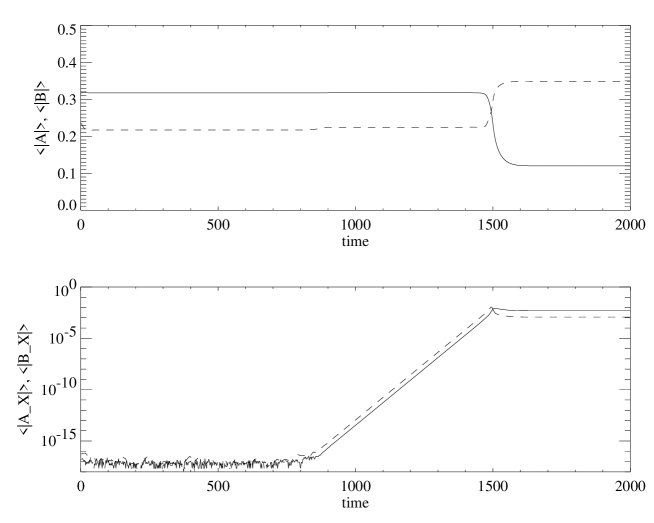
Figure 5: Time evolution of perturbation from the $M_{+}$ equilibrium near $\mathbb{X}$. $\mu_{1}=0.018$, $\mu_{2}=0.7$; all other coefficients are as in figure 1.The four panels show spatial averages of: (a) $|A|$ (solid line) and $|B|$ (dashed line), (b) $|A_{X}|$ (solid) $|B_{X}|$ (dashed), (c) $\chi$ (solid), $\theta$ (dashed), (d) $|\raise 2.0pt\hbox{$\chi$}_{X}|$ (solid), $|\theta_{X}|$ (dashed). An initial transient growth of a TW mode (illustrated by the constant rate of evolution of $\theta$ for $900<t<1500$) gives way to a spatially-modulated steady state at $t=1600$.

The final state is, however, steady, and consists of an extremely long-wavelength, but $O(1)$ in amplitude, modulation - see figure 6. Throughout most of the domain $\theta$ and $\phi$ increase linearly with $X$, while $\chi$ remains close to zero.

Figure 6: Steady spatially-modulated state reached at the end of the numerical integration illustrated in figure 5. $\mu_{1}=0.018$, $\mu_{2}=0.7$; all other coefficients are as in figure 1. (a) $|A|$ (solid), $|B|$ (dashed). (b) $\chi$ (solid), $\theta$ (dashed).

From the form of the equations (8) - (11) it is clear that families of solutions with $\theta_{X}$ and $\phi_{X}$ constant and non-zero are possible, corresponding to exactly spatially-periodic states with wavenumber close to unity. Some analytic investigation of these solutions should be possible. It may well be possible also to look analytically at other classes of solution, for example homoclinic orbits corresponding to spatially localised structures in infinite domains, or solutions where $R$ and $S$ are spatially periodic, but the possibilities are too numerous to discuss further here.

5.4 Dynamics near the codimension-two point $\mathbb{Y}$

Below the point $\mathbb{A}$ on figure 1 the LW and SW curves intersect at yet another codimension-two point, labelled $\mathbb{Y}$ on figure 1(a). A similar analysis to that near $\mathbb{X}$ could be carried out here, leading to a pair of equations for the SW instability (which leads to time-periodic variations in solution amplitude), and the LW (phase) instability. Although we have not computed the reduced ‘normal form’ in this case, its structure is simple to derive and we include it for completeness. The relevant reduced equations describing the dynamics of this bifurcation are coupled ODEs for two variables $(z,\theta)$ where $z\in\mathbb{C}$ gives the perturbation in the direction of the SW instability and $\theta\in\mathbb{R}$ describes the LW instability. On symmetry grounds, the equations will be invariant under the transformation $(z,\theta,\partial_{X})\rightarrow(z,-\theta,-\partial_{X})$. We also make use of the normal form symmetry $z\rightarrow\mathrm{e}^{\mathrm{i}\psi}z$ which appears naturally in Hopf bifurcation problems, and we use the fact that only spatial derivatives of $\theta$ will appear because the value of $\theta$ itself is dynamically unimportant. Under these constraints the reduced equations (including terms up to cubic order in $(z,\theta,\partial_{X})$) take the form

$$\dot{z} = (\lambda_{1}+\mathrm{i}\omega)z-\xi_{0}z|z|^{2}+\xi_{1}z\theta_{X}+\xi_{2}z_{XX},$$ (63)

$$\dot{\theta} = -\lambda_{2}\theta_{XX}-\xi_{3}\theta_{XXXX}+\mathrm{i}\xi_{4}\left(z_{X}\bar{z}-\bar{z}_{X}z\right)+\xi_{5}|z|^{2}_{X},$$ (64)

where $\xi_{0},\xi_{1},\xi_{2}\in\mathbb{C}$ and $\xi_{3},\xi_{4},\xi_{5}\in\mathbb{R}$ are undetermined coefficients, $\omega>0$ is the frequency of oscillation at the Hopf bifurcation, and $\lambda_{1}$, $\lambda_{2}$ are real bifurcation parameters. Due to the large number of undetermined coefficients, space does not permit a detailed investigation of this bifurcation here. However, since the symmetry does not permit a linear term in $z$ in the $\dot{\theta}$ equation it is clear that the dynamics of (63) - (64) are not related to those of (53) and (56). The codimension-one bifurcation that occurs for $\lambda_{1}=0$ and $\lambda_{2}<0$ was one of the ‘normal forms’ identified by Coullet & Iooss [4] and has been explored numerically by Lega [16] and Daviaud et al. [10]. In particular, these authors identify two distinct regimes of spatio-temporal chaos depending on the choices of the coupling coefficients in (63) - (64).

5.5 Instability of $M_{-}$ to long-wavelength perturbations

Finally in this section, we briefly discuss the dynamics in the quadrant $\mu_{1}>0$, $\mu_{2}<0$. The spatially-periodic equilibrium state $M_{-}$ exists in the whole of this region and is stable when $\mu_{2}$ is sufficiently negative, for a fixed $\mu_{1}>0$. The amplitudes $R=R_{0}$ and $S=S_{0}$ satisfy

$$0 = \mu_{1}-q^{2}-S_{0}-a_{1}R_{0}^{2}-b_{1}S_{0}^{2},$$ (65)

$$0 = \mu_{2}S_{0}+R_{0}^{2}-a_{2}S_{0}^{3}-b_{2}R_{0}^{2}S_{0},$$ (66)

and $\raise 2.0pt\hbox{$\chi$}=\pi$. For $q=0$, $M_{-}$ states lose stability to TW solutions as $\mu_{2}$ is increased at fixed positive $\mu_{1}$. These TW states have $\raise 2.0pt\hbox{$\chi$}\approx\pi$ near the bifurcation since $\raise 2.0pt\hbox{$\chi$}=\pi$ for $M_{-}$. As for $M_{+}$ this phase instability also generates a distinct long-wavelength instability when $q\neq 0$.

Following the usual linearisation of (8) - (11) about $M_{-}$ we find that a long-wavelength instability occurs when

$$(2cS_{0}^{2}-R_{0}^{2})(2S_{0}^{3}(b_{1}b_{2}-a_{1}a_{2})+(b_{2}-2b_{1})S_{0}^{2}-S_{0}-a_{1}R_{0}^{2}) = 2q^{2}(R_{0}^{2}+2a_{2}S_{0}^{3}).$$

Since the bifurcation to TW occurs when $R_{0}^{2}=2S_{0}^{2}$ as before, it is clear that in the case $c=1$ these bifurcation curves do not intersect and no further codimension-two bifurcation points appear. In the limit where we keep $\mu_{1}\sim O(1)$ fixed and let $\mu_{2}\rightarrow-\infty$ we see from (65) - (66) that $S_{0}\rightarrow 0$ and $R_{0}\sim O(1)$. Then (LABEL:m_minus_lw) is satisfied when $a_{1}R_{0}^{2}\approx 2q^{2}$ to leading order. From (65) this gives the asymptotic behaviour of the curve of LW instability: $\mu_{1}\sim 3q^{2}$, illustrated in figure 7.

Figure 7: Region of stability of the mixed mode $M_{-}$ for the illustrative set of coefficients $a_{1}=1$, $a_{2}=5$, $b_{1}=2$, $b_{2}=0$, $c=1$, $q=0.2$. The region of stable $M_{-}$ is bounded by TW (solid line) and LW (dash-dotted line) instabilities. Note the asymptotic behaviours of the LW curve: at large negative $\mu_{2}$ we find $\mu_{1}\sim 3q^{2}=0.12$ for this set of coefficients; at large $\mu_{1}$ it closely follows the TW curve.

In summary, in this section we have identified various codimension-one and two bifurcations involving modulational instabilities. In particular, two codimension-2 points, $\mathbb{X}$ and $\mathbb{Y}$, organise the interaction of the new LW instability with the previously-studied TW and SW bifurcations. Reductions of the original PDEs (6) - (7) to ‘normal form’ equations describing the dynamics near these bifurcations enables us to gain insight into the nature of these bifurcations, despite the fact that solutions, even of the reduced equations, may have extremely complicated spatial structure.

6 The heteroclinic cycle

One of the most interesting features of the ODE problem (12) - (14) analysed in Part 1 is the existence of a robust heteroclinic cycle between pure mode solutions related by a half-wavelength spatial translation; for example $P_{+}$ and $P_{-}$. For the coefficient values selected in this paper this heteroclinic cycle exists for an open region of the $(\mu_{1},\mu_{2})$ plane, abutting the origin. Its formation relies on the existence of pairs of two-dimensional invariant subspaces for the dynamics: for example within the two-dimensional subspace $\mathrm{Fix}(m_{x})=\{Im(A)=Im(B)=0\}$ the point $P_{+}$ is a saddle and $P_{-}$ is a sink and, if various other conditions are met, a connecting trajectory between them exists. The second connection is then forced to exist by symmetry, and is contained within the subspace $\mathrm{Fix}(m_{x}\circ\tau_{\pi})=\{Re(A)=Im(B)=0\}$.

For small positive $\mu_{2}$ and increasing $\mu_{1}$ the cycle is formed after a global bifurcation that involves the intersection of the unstable manifold of $P_{+}$ and the stable manifold of the origin; this bifurcation also creates or destroys the SW periodic orbit. At larger values of $\mu_{2}$ the connecting trajectory appears after a saddle-node bifurcation marking the boundary of existence of a further two $M_{+}$ equilibria. Hence this curve of saddle-node bifurcations also bounds the region of existence of the cycle. At larger $\mu_{1}$ the cycle ceases to exist where the pure mode equilibria $P_{\pm}$ gain stability in a pitchfork bifurcation with $M_{-}$ equilibria. These bifurcations proscribe the region of existence of the cycle. Within this region of existence, a further curve separates regions where it is stable or unstable. At this stability boundary a branch of modulated waves (MW) bifurcate from the cycle in a global (‘resonant’) bifurcation. Theoretical work by Armbruster et al. [1] and by Proctor & Jones [23] was confirmed by the general stability results of Krupa & Melbourne [14, section 6.1]. It turns out that the natural condition (that the ratio of eigenvalues in the ‘contracting’ and ‘expanding’ directions should be greater than one for stability) is necessary and sufficient. This yields the condition $\mu_{1}<b_{1}\mu_{2}/a_{2}$ for the stability boundary of the cycle.

When modulational terms are included, the instability of $P_{+}$ to $P_{-}$ that is necessary for existence of the cycle implies that $P_{+}$ will also be unstable to sufficiently long-wavelength perturbations, so it might be expected that the cycle also could not be stable to long-wavelength perturbations. Moreover, the subspaces $\{Im(A)=Im(B)=0\}$ and $\{Re(A)=Im(B)=0\}$ are no longer invariant for the dynamics; spatial variations of the amplitude $A$ drive the evolution of the phase $\theta$ when $q\neq 0$, see equation (9). Of course, the cycle still exists, within the subspace of solutions with no spatial modulation at all. But, in large domains it cannot be asymptotically stable (that is, points in a full neighbourhood - in some appropriate sense - of the cycle converge to it) as the equilibria $P_{\pm}$ will be unstable to perturbations of a sufficiently long wavelength, as well as to each other within the subspaces containing the heteroclinic connecting orbits.

Numerical simulations show that spatially-modulated perturbations eventually grow, when $q\neq 0$, and the simulation converges to a periodic orbit rather than showing the characteristic increases of time spent near each equilibrium that would indicate convergence to the robust heteroclinic cycle.

In this section we analyse the behaviour of trajectories close to the cycle using a linearised stability analysis near the equilibria $P_{\pm}$ and under the commonly-used assumption that trajectories near the cycle spend very little time passing between neighbourhoods of the equilibria. Our aim is to determine conditions for existence of periodic orbits lying close to the cycle. We restrict our attention to periodic orbits that spend equal amounts of time near each equilibrium since this feature is observed in numerical work.

Recall from section 4 that the linear stability of $P_{+}$ to perturbations $\sim\alpha_{1}\mathrm{e}^{\mathrm{i}\ell X}+\bar{\alpha}_{2}\mathrm{e}^{-\mathrm{i}\ell X}$ in $A(X,T)$ with wavenumber $\ell$ is given by the matrix (LABEL:pplus_linear) acting on the amplitudes $(\alpha_{1},\alpha_{2})$. For simplicity we write this matrix as

$$M_{1} = \left(\begin{array}[]{cc}a_{0}-\hat{q}&b_{0}\\ b_{0}&a_{0}+\hat{q}\\ \end{array}\right),$$ (70)

where

$$a_{0} = \mu_{1}-q^{2}-b_{1}B_{0}^{2}-\ell^{2},$$ (71)

$$b_{0} = B_{0},$$ (72)

$$\hat{q} = 2q\ell.$$ (73)

Note that a necessary condition for the existence of the cycle is that the eigenvalues $\lambda_{\pm}$ of $M_{1}$, when evaluated when $\ell=0$, satisfy $\lambda_{-}<0<\lambda_{+}$, so that $P_{+}$ is a saddle point. The form of $M_{1}$ implies that this is equivalent to requiring $a_{0}<0$ when $\ell=0$, and hence in the rest of this section we assume $a_{0}<0$. The corresponding linearisation around $P_{-}$ is denoted $M_{2}$:

$$M_{2} = \left(\begin{array}[]{cc}a_{0}-\hat{q}&-b_{0}\\ -b_{0}&a_{0}+\hat{q}\\ \end{array}\right).$$ (76)

The form of $M_{2}$ is determined entirely from $M_{1}$ and the equivariance of the ODEs (6) - (7).

We assume that trajectories close to the heteroclinic cycle spend equal amounts of time $T$ near each equilibrium, and that we may ignore the time spent travelling between neighbourhoods of the equilibria. Hence a perturbation $v_{0}=(\alpha_{1},\alpha_{2})^{T}$ near $P_{+}$ evolves to the point

$$v_{1} = \mathcal{S}v_{0}=\exp(M_{2}T)\exp(M_{1}T)v_{0},$$

where the matrix $\mathcal{S}$ is given by

$$\mathcal{S} = \frac{1}{2c_{0}^{2}}\left(\begin{array}[]{cc}2b_{0}^{2}e_{+}e_{-}+\hat{q}e_{+}^{2}(q-c_{0})+qe_{-}^{2}(q+c_{0})&-b_{0}q(e_{+}-e_{-})^{2}\\ b_{0}q(e_{+}-e_{-})^{2}&2b_{0}^{2}e_{+}e_{-}+qe_{+}^{2}(q+c_{0})+qe_{-}^{2}(q-c_{0})\end{array}\right),$$ (79)

and $c_{0}=\sqrt{\hat{q}^{2}+b_{0}^{2}}$ and $e_{\pm}=\exp[(a_{0}\pm c_{0})T]$. The eigenvalues of $\mathcal{S}$ then determine the stability of the cycle. We are particularly interested in the dependence of these eigenvalues on the travel time $T$, the selected wavelength $\ell$ and the wavenumber mismatch parameter $q$.

When $q=0$, $\mathcal{S}$ simplifies enormously: it is diagonal with eigenvalues $e_{+}e_{-}=\exp(2a_{0}T)$ where $a_{0}$ is defined in (71). Since $a_{0}<0$ we have contraction of the perturbation vector $v_{0}$ under successive iterates of $\mathcal{S}$. This corresponds to trajectories passing repeatedly through neighbourhoods of $P_{\pm}$, and converging to the cycle. This result is independent of the time $T$ spent near each equilibrium.

For general $q\neq 0$ the eigenvalues of $\mathcal{S}$ will, however, depend on $T$. Moreover, for any $q\neq 0$, $\mathcal{S}$ will have eigenvalues of modulus greater than unity when $T$ is taken to be sufficiently large (so that $e_{+}$ is sufficiently large). So, in addition to the discussion above, we can conclude directly from the form of the map that for any non-zero $q$ the cycle is unstable.

Numerical simulations indicate that trajectories remain close to the cycle, though, so it is natural to ask whether stable dynamics close to the cycle is possible. One possibility is the existence of a long-period periodic orbit. That such an orbit might exist is motivated by the observation that $\mathcal{S}$ has an eigenvalue greater than unity for $T\gg 1$, i.e. trajectories very close to the cycle are pushed further away from it, but that for $T\sim 1$ the eigenvalues of $\mathcal{S}$ may lie within the unit circle, indicating that trajectories that start further away from the cycle move closer on successive passes near the cycle. This behaviour is confirmed by numerical simulations (see figure 8), where we choose an initial condition lying extremely close to the subspace of non-modulated solutions, but not close to the heteroclinic cycle.

Figure 8: Temporal evolution of the first few Fourier modes (writing $A(X,T)=\sum_{j=0}^{N}\hat{A}_{j}\mathrm{e}^{2\pi\mathrm{i}j/L}$ and $B(X,T)$ similarly) in a solution starting near the subspace of non-modulated solutions and converging to the periodic orbit. The top graph shows the time evolution of $|\hat{A}_{0}|$ (dashed) and $|\hat{B}_{0}|$ (solid). The other three graphs show $|\hat{A}_{j}|$ (dashed) and $|\hat{B}_{j}|$ (solid) for $j=1,2,3$ respectively.Note the initial decay when the travel time $T$ is short, followed by growth of the perturbation as $T$ increases.Parameter values are $L=30$, $\mu_{1}=10^{-6}$, $\mu_{2}=0.1$, $q=10^{-3}$, and the coefficients are as in figure 1.

Thus the first few travel times $T$ between neighbourhoods of $P_{\pm}$ occur with $T$ small, and the perturbation decays. Then, as the trajectory becomes closer to the cycle $T$ increases and the perturbation grows (exponentially on average) until the trajectory converges to the periodic orbit.

The above argument is unusual in that it suggests that we can extract nonlinear information (about the period of the orbit) from a purely linear calculation (that which leads to the form of $\mathcal{S}$). This is because we are essentially using $T$ as a proxy for the closest distance between the periodic orbit and the heteroclinic cycle. Hence solving for the position of the orbit and solving for $T$ are really the same thing. By setting up the usual ‘small box’ approach we could construct a return map, fixed points of which would correspond to periodic orbits. By using $T$ instead, we are able to circumvent the need to compute this return map in full in order to extract an estimate for the period. Essentially we construct the component of the return map in a pair of directions orthogonal to the invariant plane corresponding to unmodulated solutions. Then the condition for locating a fixed point of this part of the map is identical to the condition that $\mathcal{S}$ has an eigenvalue of $+1$.

At least for small $q$ and large times $T$ we expect that the behaviour outlined above could be captured by the map $\mathcal{S}$ based on linearisation near $P_{\pm}$. We compute the approximate period $P(q)\approx 2T(q)$ of a stable periodic orbit by imposing the condition that the larger eigenvalue $m_{+}$ of $\mathcal{S}$ is $+1$ (the other ($m_{-}$) lies inside the unit circle). Finally we consider only the minimum wavenumber $\ell_{min}=2\pi/L$ since this is the mode with the highest growth rate for the points in the $(\mu_{1},\mu_{2})$ plane that we consider. Hence the eigenvalue condition yields a relationship (implicitly) between $T$ and $q$ which can be compared with numerical simulations. This relationship simplifies in the asymptotic regime where $q$ is small and $T$ is large.

Substituting for $e_{\pm}=\exp[(a_{0}\pm c_{0})T]$ in $\mathcal{S}$ and computing its eigenvalues we find

$$m_{\pm} = \frac{\left[2b_{0}^{2}\mathrm{e}^{2c_{0}T}+\hat{q}^{2}\mathrm{e}^{4c_{0}T}+\hat{q}^{2}\pm Y\right]\mathrm{e}^{2a_{0}T}}{2(b_{0}^{2}+\hat{q}^{2})\mathrm{e}^{2c_{0}T}},$$ (80)

where

$$Y^{2} = 4\hat{q}^{2}b_{0}^{2}\mathrm{e}^{6c_{0}T}+4\hat{q}^{2}b_{0}^{2}\mathrm{e}^{2c_{0}T}+\hat{q}^{4}\mathrm{e}^{8c_{0}T}-2\hat{q}^{4}\mathrm{e}^{4c_{0}T}+\hat{q}^{4}-8\hat{q}^{2}b_{0}^{2}\mathrm{e}^{4c_{0}T}.$$

It might appear that the dominant term for large $T$ is the first term in the expression for $Y^{2}$, proportional to $\hat{q}^{2}\mathrm{e}^{6c_{0}T}$, but this is incorrect. In fact, the dominant terms in the limit of small $\hat{q}$ and large $T$ are those proportional to $\hat{q}^{2}\mathrm{e}^{4c_{0}T}$. This leads to the asymptotic relationship

$$T \sim \frac{1}{a_{0}+b_{0}}\log\left(\frac{b_{0}}{\hat{q}}\right),$$

as $q\rightarrow 0$. For two combinations of $L$ and $\mu_{2}$, figure 9 compares this asymptotic relationship with the exact implicit $T$–$q$ relationship implied by (80) setting $m_{+}=1$, and with the results of numerical integrations of the PDEs (6) - (7). In both cases there is clear agreement as long as $q$ is sufficiently small. At small $q$ the numerical simulations become more difficult, due to the intermittent nature of the dynamics.

Figure 9: The dependence on $q$ of the approximate half-period $T(q)$ of the periodic orbit near the heteroclinic cycle, for two combinations of $L$ and $\mu_{2}$. In both cases, the illustrative coefficient values were used, as for figure 1, and $\mu_{1}=q^{2}$. Squares ($\Box$) are the results of numerical simulations for $L=30$ and $\mu_{2}=0.1$, and triangles ($\triangle$) are numerical results for $L=25$, $\mu_{2}=0.05$. Diamonds $(\Diamond$) give the exact $T$–$q$ relationship implied by the linearised analysis near the cycle using $\ell=\ell_{min}=2\pi/L$, in both cases, and the asymptotic result of the linearised analysis is shown by the dashed and solid lines.

Given the several approximations involved in the analytic estimate of $T(q)$ the results of figure 9 are enouraging. The major discrepancy in the analysis is the consideration of only one wavenumber $\ell_{min}=2\pi/L$ in the estimate. Implicitly we assume that the ‘most unstable’ eigenfunction direction near $P_{+}$ is aligned exactly with the single Fourier mode $\mathrm{e}^{\mathrm{i}\ell_{min}X}$.

For larger $q$ numerical simulations did not converge to a stable periodic orbit, but instead remained spatiotemporally disordered even after large integration times. Although solutions still often spend considerable amounts of time near the spatially-uniform $P_{+}$ state these events occur only intermittently. At much larger $q$, numerical integrations of the PDEs show that the cycle still plays a rôle in local organisation of the spatiotemporally complicated dynamics. The spatial structure of solutions often resembles a series of fronts between intervals of points which remain near either $P_{+}$ or $P_{-}$ for a time, and then switch rapidly to a neighbourhood of the other equilibrium. This is illustrated in figure 10, particularly around $X=90$ and $X=140$ (where the solution is close to $P_{+}$), and at $X=120$ where the solution is close to $P_{-}$. For the parameter values of the figure, the pure mode equilibria have amplitude $|B|=0.2$. Nearby spatial locations are often still well-correlated in time, see figure 11.

Figure 10: The moduli $|A|$ (dashed line) and $|B|$ (solid line) for an instantaneous view of a typical solution of the PDEs (6) - (7). The horizontal dash-dotted line is at $|B|=\sqrt{(}\mu_{2}/a_{2})=0.2$ corresponding to the amplitude of the $P_{+}$ equilibrium. The parameter values are $q=0.2$, $\mu_{1}=0.04$ and $\mu_{2}=0.2$; the illustrative coefficient values are used and the domain is of length $L=200$ with periodic boundary conditions.

Figure 11: Time evolution of $|B|$ at two spatial locations, $X=105$ (solid line) and $X=110$ (dashed line), for a typical solution of the PDEs (6) - (7). The parameter values, coefficients and domain size are as for figure 10.

7 Stable travelling waves and complex spatiotemporal dynamics

At large positive $\mu_{1}$ and $\mu_{2}$ the TW states are restabilised after a Hopf bifurcation involving a branch of modulated waves generated by the global bifurcation in which the heteroclinic cycle loses stability. Surprisingly, for the spatially-extended system, these spatially-homogeneous TW states are also stable for large enough $\mu_{1}$ and $\mu_{2}$, as shown in figures 12 and 13.

Figure 12: Temporal evolution of the spatial averages of the amplitude and phase variables at $\mu_{1}=0.15$, $\mu_{2}=0.7$, $L=30$; all other coefficients are as in figure 1. The four panels show spatial averages of: (a) $|A|$ (solid line) and $|B|$ (dashed line); (b) $|A_{X}|$ (solid) $|B_{X}|$ (dashed); (c) $\chi$ (solid), $\theta$ (dashed); (d) $|\raise 2.0pt\hbox{$\chi$}_{X}|$ (solid), $|\theta_{X}|$ (dashed). After an oscillatory transient the solution is attracted towards a spatially-periodic TW state where $\theta$ (and $\phi$, not shown) increase linearly with time while $|A|$, $|B|$ and $\chi$ remain constant.

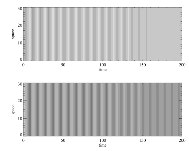
Figure 13: The spatio-temporal evolution of the amplitudes $|A|$ (upper panel) and $|B|$ (lower panel) for the parameter values of figure 12, showing convergence to TW.

The stable TW coexist with stable complicated spatiotemporal dynamics, illustrated in figures 14 and 15. The latter state might be expected to be a more generic solution in this region of the $(\mu_{1},\mu_{2})$ plane, although no systematic study of the relative sizes of the basins of attraction has been performed.

Figure 14: Temporal evolution of a persistent complex spatiotemporal state at $\mu_{1}=0.15$, $\mu_{2}=0.7$, $L=30$; all other coefficients are as in figure 1. The four panels show spatial averages of: (a) $|A|$ (solid line) and $|B|$ (dashed line); (b) $|A_{X}|$ (solid) $|B_{X}|$ (dashed); (c) $\chi$ (solid), $\theta$ (dashed); (d) $|\raise 2.0pt\hbox{$\chi$}_{X}|$ (solid), $|\theta_{X}|$ (dashed). This solution coexists stably with the TW state shown in figure 12.

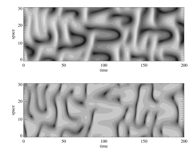
Figure 15: Spatio-temporal evolution of the amplitudes $|A|$ (upper panel) and $|B|$ (lower panel) for the parameter values of figure 14, showing complicated spatiotemporal dynamics.

8 Discussion and conclusions

In this paper we have examined the robustness of the results of Part 1 on the dynamics near the $1:2$ strong spatial resonance, to modulational instabilities which might be expected to play a role when the spatial resonance is close to, but not exactly, $1:2$. We have derived a pair of coupled amplitude equations using symmetry arguments; these amplitude equations are PDEs rather than ODEs as is the case for exact resonance.

We have examined the stability of the spatially-periodic solutions found in Part 1, looking for instabilities to finite-wavelength and long-wavelength perturbations. In general, we find that the results of Part 1 still apply when $\mu_{1}$ and $\mu_{2}$ are large (equivalently when the mismatch $q$ is small), but that new instabilities are present near the codimension-two point $\mu_{1}=\mu_{2}=0$. Since these lead, in general, to variations with a horizontal wavenumber $\mathcal{O}(\varepsilon q)$, solutions still resemble those of the non-modulated problem over short lengthscales.

This paper is primarily concerned with identifying the several codimension-two points in the parameter space which link modulational instabilities and amplitude or phase instabilities which are present in the ODEs discussed in Part 1. We have presented reduced equations that describe the dynamics near these various points. The form of these reduced equations (which are still PDEs) may be deduced from symmetry arguments, and can also be derived through perturbation expansions. This analysis enables us to understand qualitative features of the dynamics; although analytic solutions are still extremely difficult to derive for the reduced equations, this process of deriving ‘normal forms’ contributes greatly to an understanding of the interaction of these various instabilities.

Our three main results are firstly, that the pure mode $P$ and the mixed-mode $M_{+}$ may undergo steady-state instabilities to finite-wavelength modes with a maximum critical wavenumber $\ell_{c}=q$ (for $P$) and $\ell_{c}=2q$ (for $M_{+}$). This confirms our intuition; it is natural to think that there are only two important lengthscales in the problem - the $O(1)$ lengthscale of the spatially-periodic patterns and long lengthscales $>O(1/\varepsilon q)$ introduced by the deviation from exact resonance. $M_{+}$ may also undergo an oscillatory bifurcation to a non-zero wavenumber mode, and numerical investigations suggest this wavenumber is also $O(q)$. Secondly, the reduction of the governing PDEs to a ‘normal form’ and subsequent analysis of these reduced equations for the codimension-two phase instability at the point $\mathbb{X}$ is novel and is presented in detail. Thirdly, we have considered the fate of the structurally stable heteroclinic cycle present in the ODE problem. Although the equilibria on the cycle, and hence the cycle itself, must be unstable to long-wavelength perturbations, the dynamics for small $q$ result in a stable periodic orbit that lies close to the cycle and whose period can be estimated well analytically. At larger $q$ the heteroclinic cycle still organises the spatial dynamics over short distances, although solutions are spatiotemporally complex as might in general be expected.

There is, of course, much more work that could be done on this problem. Two obvious directions of interest are the fate of the more complicated heteroclinic cycles examined by Porter & Knobloch [20] to modulational perturbations, and the behaviour for asymptotically large $q$ (within this scaling ansatz); we have concentrated on behaviour for $q\leq 1$, where the results may be most easily interpreted with reference to previous work.

Appendix

In this appendix we give the coefficients in the Ginzburg–Landau equation governing the instability of the pure mode solution $P_{+}$ along the interior of the line $\mathbb{O}\mathbb{L}$, discussed in section 4.

The $P_{+}$ equilibrium is given by $A=0$, $B=\sqrt{\mu_{2}/a_{2}}=B_{0}$. We start from the ansatz

$$A(X,T) = \varepsilon\left[\alpha(\xi,\tau)B_{0}\mathrm{e}^{\mathrm{i}\ell X}+\bar{\alpha}(\xi,\tau)2q(q+\ell)\mathrm{e}^{-\mathrm{i}\ell X}\right]$$ (81)

$$+\varepsilon^{2}\left[\gamma_{0}(\xi,\tau)+\gamma_{1}(\xi,\tau)\mathrm{e}^{2\mathrm{i}\ell X}+\gamma_{2}(\xi,\tau)\mathrm{e}^{-2\mathrm{i}\ell X}\right]+O(\varepsilon^{3}),$$

$$B(X,T) = B_{0}+\varepsilon^{2}\left[\beta_{0}(\xi,\tau)+\beta_{1}(\xi,\tau)\mathrm{e}^{2\mathrm{i}\ell X}+\beta_{2}(\xi,\tau)\mathrm{e}^{-2\mathrm{i}\ell X}\right]+O(\varepsilon^{3}),$$ (82)

where $\xi=\varepsilon X$ is a new, longer, lengthscale and $\tau=\varepsilon^{2}T$ is a new slower timescale. After a multiple-scales expansion, substituting this ansatz into the PDEs (6) - (7), the perturbation amplitudes $\beta_{0},\beta_{1},\beta_{2},\gamma_{0},\gamma_{1},\gamma_{2}$ can be expressed in terms of $\alpha$. The usual solvability condition at $O(\varepsilon^{2})$ is satisfied identically, and at $O(\varepsilon^{3})$ the solvability condition yields the Ginzburg–Landau amplitude equation for $\alpha$:

$$\hat{c}_{1}\alpha_{\tau} = \hat{c}_{1}\alpha_{\xi\xi}-\hat{c}_{2}\alpha|\alpha|^{2},$$

where the real coefficients $\hat{c}_{1}$ and $\hat{c}_{2}$ are

$$\hat{c}_{1} = B_{0}^{2}+4q^{2}(q+\ell)^{2},$$

$$\hat{c}_{2} = a_{1}[B_{0}^{4}+16q^{4}(q+\ell)^{4}+16B_{0}^{2}q^{2}(q+\ell)^{2}]$$

$$+\hat{c}_{3}B_{0}[2b_{1}B_{0}^{2}+8q^{2}(q+\ell)^{2}b_{1}-4q(q+\ell)]$$

$$+4b_{1}B_{0}^{2}q(q+\ell)(\hat{c}_{4}+\hat{c}_{5})-B_{0}^{2}\hat{c}_{4}-4q^{2}(q+\ell)^{2}\hat{c}_{5},$$

$$\hat{c}_{3} = -[B_{0}^{2}b_{2}+4b_{2}q^{2}(q+\ell)^{2}+4q(q+\ell)]/(2a_{2}B_{0}),$$

$$\hat{c}_{4} = \frac{2B_{0}^{2}q(q+\ell)[a_{2}q(q+\ell)-4b_{2}c\ell^{2}]-B_{0}^{2}(a_{2}B_{0}^{2}+4c\ell^{2})}{8c\ell^{2}(a_{2}B_{0}^{2}+2c\ell^{2})},$$

$$\hat{c}_{5} = \frac{a_{2}B_{0}^{4}-2q(q+\ell)[q(q+\ell)(a_{2}B_{0}^{2}+c\ell^{2})+4b_{2}B_{0}^{2}c\ell^{2}]}{8c\ell^{2}(a_{2}B_{0}^{2}+2c\ell^{2})}.$$

Hence $\hat{c}_{2}>0$ when $a_{1}$ is sufficiently positive. In the special case $\hat{c}_{3}=\hat{c}_{4}=\hat{c}_{5}=0$, the expression for $\hat{c}_{2}$ agrees with that derived by Coullet et al. [6]. In fact, the $O(\varepsilon^{2})$ amplitudes $\gamma_{0},\gamma_{1},\gamma_{2}$ in (81) do not contribute to the complexity of the expression for $\hat{c}_{2}$; the complexity is derived from the third-order contributions from the $\dot{B}$ equation.

References

- [1] D. Armbruster, J. Guckenheimer & P. Holmes, Heteroclinic cycles and modulated travelling waves in systems with O(2) symmetry. Physica D 29, 257–282 (1987)
- [2] G.J.B. van den Berg, Dynamics and equilibria of fourth order differential equations. PhD Thesis, Leiden University (2000)
- [3] P. Coullet, C. Elphick & D. Repaux, Nature of spatial chaos. Phys. Rev. Lett., 58, 431–434 (1987)
- [4] P. Coullet & G. Iooss, Instabilities of one-dimensional cellular patterns Phys. Rev. Lett. 64, 866–869 (1990)
- [5] P. Coullet & D. Repaux, Models of pattern formation from a singularity theory point of view, in Instabilities and Nonequilibrium structures, eds E. Tirapegui and D. Villarroel pp179–195. D. Reidel (1987)
- [6] P. Coullet, D. Repaux & J.M. Vanel, Quasiperiodic patterns. In Contemporary Mathematics, 56 19–29. AMS (Providence) (1986)
- [7] S.M. Cox, Mode interactions in Rayleigh–Bénard convection. Physica D 95, 50–61 (1996)
- [8] M. Cross & P.C. Hohenberg, Pattern formation outside of equilibrium Rev. Mod. Phys., 65, 851–1112 (1993)
- [9] G. Dangelmayr, Steady-state mode interactions in the presence of -symmetry. Dyn. Stab. Syst., 1 159–185 (1986)
- [10] F. Daviaud, J. Lega, P. Bergé, P. Coullet & M. Dubois, Spatiotemporal intermittency in a 1D convective pattern - theoretical-model and experiments. Physica D 55, 287–308 (1992)
- [11] M. Higuera, H. Riecke & M. Silber, Near-resonant, steady mode interaction: periodic, quasi-periodic and localised patterns. Preprint (2003)
- [12] K. Julien, Strong spatial resonance in convection. PhD Thesis, University of Cambridge (1991)
- [13] C.A. Jones & M.R.E. Proctor, Strong spatial resonances and travelling waves in Bénard convection. Phys. Lett. A 121, 224–228 (1987)
- [14] M. Krupa & I. Melbourne, Asymptotical stability of heteroclinic cycles in systems with symmetry. Erg. Theor. & Dynam. Sys., 15, 121–147 (1995)
- [15] A.S. Landsberg & E. Knobloch, New types of waves in systems with symmetry. Phys. Lett. A 179, 316–324 (1993)
- [16] J. Lega, Secondary Hopf bifurcation of a one-dimensional periodic pattern. Eur. J. Mech. B/Fluids 10, Suppl. 145–150 (1991)
- [17] I. Melbourne, Steady-state bifurcation with Euclidean symmetry. Trans. A.M.S. 351, 1575–1603 (1999)
- [18] I. Mercader, J. Prat & E. Knobloch, Robust heteroclinic cycles in two-dimensional Rayleigh-Bénard convection without Boussinesq symmetry. Int. J. Bif. Chaos 12, 2501–2522 (2002)
- [19] L.A. Peletier & W.C. Troy, Chaotic spatial patterns described by the Extended Fisher-Kolmogorov equation. J. Diff. Eqns., 129, 458–508 (1996)
- [20] J. Porter & E. Knobloch, New type of complex dynamics in the 1:2 spatial resonance. Physica D, 159, 125–154 (2001)
- [21] J. Prat, I. Mercader & E. Knobloch, The mode interaction in Rayleigh-Bénard convection with and without Boussinesq symmetry. Int. J. Bif. Chaos 12, 281–308 (2002)
- [22] M.R.E. Proctor & J.H.P. Dawes, Turing instabilities induced by strong spatial resonance. In preparation.
- [23] M.R.E. Proctor & C.A. Jones, The interaction of two spatially resonant patterns in thermal convection. Part 1. Exact 1:2 resonance. J. Fluid Mech. 188, 301–355 (1988)
- [24] S. Ya. Vyshkind & M.I. Rabinovich, The phase stochastization mechanism and the structure of wave turbulence in dissipative media. Sov. Phys. JETP 44, 292–299 (1976)