Information Flow through a Chaotic Channel: Prediction and Postdiction at Finite Resolution

Abstract

We reconsider the persistence of information under the dynamics of the logistic map in order to discuss communication through a nonlinear channel where the sender can set the initial state of the system with finite resolution, and the recipient measures it with the same accuracy. We separate out the contributions of global phase space shrinkage and local phase space contraction and expansion to the uncertainty in predicting and postdicting the state of the system. Thus, we determine how the amplification parameter, the time lag, and the resolution influence the possibility for communication. A novel representation for real numbers is introduced that allows for a visualization of the flow of information between scales.

I Introduction

When observing a dynamical system in a given state, one can ask several basic questions, two of which are, “Where did it come from?” and “Where is it going?” These questions are especially relevant when one wants to communicate a message by setting the initial state of a system, whose state at a later time is then detected by the recipient of the message. If the final state is completely uncertain, the message is lost – this is often the case in chaotic systems. On the other hand, if all initial states converge to one final state, the recipient cannot determine what message he was to receive – this can occur in dissipative systems. Many nonlinear systems have elements of both chaos and dissipation; as an example, we choose the logistic map $f(x)=ax(1-x)$ Ott (1993). We determine the relevance of state space shrinkage and expansion for all values of the amplification parameter $a$, and discuss to what extent communication in the sense mentioned is possible. Note that using a chaotic channel is not something the sender chooses to do – he may be forced to entrust the message to an unreliable medium. This distinguishes our perspective from other publications on communication through chaos such as in Refs. Hayes et al. (1993); Pecora and Carroll (1990); Bollt et al. (1997); Rulkov et al. (2002); Baptista (1998), where chaotic dynamics are used in order to amplify and transmit small signals.

We will show that for very short time intervals between the initialization and the measurement, the chaotic regime near $a=4$ allows for optimal communication; for intermediate times, the bifurcation points offer the best chances of deciphering the message; and for long times, no information remains except in the bifurcation regime, where one can distinguish between the branches of the cycle. Under all circumstances, uncertainty about the time at which the system was initialized leads to additional losses of information.

The degree to which an observation at one time determines the result of an observation at a different time is given by the mutual information between these observations, and the conditional information between them. The relevance of measuring information to characterize the behavior of chaotic systems was realized more that 20 years ago Shaw (1981); Farmer (1982); Pompe et al. (1986); Pompe and Leven (1986); Kruscha and Pompe (1988) and discussed in various contexts Schittenkopf and Deco (1996); Deco et al. (1997); Wiegerinck and Tennekes (1990); some of the results presented here have been either alluded to or derived before, especially in Ref. Pompe et al. (1986). However, for concrete calculations, most of these references assumed that the system had already reached a stationary state or attractor, whereas relaxation to the attractor plays a crucial role in our analysis. Also, previous studies have focused on the case of fully developed chaos at $a=4$; we discuss the behavior for all regimes of $a$.

When inputs and outputs are measured with finite precision, it is useful to have a representation of numbers that separates contributions on different scales. We introduce a representation that may be superior to the usual decimal or binary representations in this regard, and use it to visualize the flow of information between scales.

Section II provides an overview of information-theoretical concepts, and a derivation of equations needed to calculate the relevant quantities for generic maps. In Sec. III, we apply the formalism to the logistic map. The possibility of transmitting messages by initializing the system is discussed in Sec. IV. In Sec. V, we introduce the clockwork representation of real numbers and use it to illustrate the dynamics of the logistic map. Section VI summarizes the results.

II Information-theory perspective

Since observations on physical systems can only be made with finite precision, the outcome can be described with a finite number of digits. Each possible distinct outcome (or elementary event) can be assigned a symbol that appears with a given probability, and Shannon’s definition of information Shannon (1948) can be applied to these symbols, resulting in a resolution-dependent, but finite, information. We divide the space of possible inputs and outputs $x\in[0,1]$ into $r$ non-overlapping bins $i$ of uniform width $1/r$, and assume that measurement precision is independent of the value endnote18 . Accordingly, we denote by $x_{i}$ the event “a trajectory starts in bin $i$,” and with $y_{j}$ the event “a trajectory ends in bin $j$.” If $x_{i}$ is drawn from a probability distribution $P_{x}(x)$, the information associated with $x$ is

$$I(x)=-\sum_{i}P_{x}(x_{i})\log_{2}P_{x}(x_{i});$$ (1)

the information $I(y)$ of $y$ can be calculated analogously from the distribution $P_{y}(y)$. The conditional information, which is needed to specify the outcome $y$ given the input $x$, is

$$I(y|x)=-\sum_{i}P_{x}(x_{i})\sum_{j}P_{y|x}(y_{j}|x_{i})\log_{2}P_{y|x}(y_{j}|x_{j}),$$ (2)

where $P_{y|x}(y_{j}|x_{i})$ denotes the conditional probability of $y_{j}$ occurring given that $x_{i}$ occurred. All other quantities (mutual information $I(x\wedge y)$, joint information $I(x,y)$, and conditional information $I(x|y)$ ) can be calculated from $I(x)$, $I(y)$, and $I(y|x)$, using the set-theoretical relations implied by Fig. 1. In particular, we make use of $I(y)=I(y\wedge x)+I(y|x)$: to specify $y$, we need the mutual information $I(y\wedge x)$, which represents information about $y$ that can be inferred from knowledge of $x$, and the conditional information $I(y|x)$.

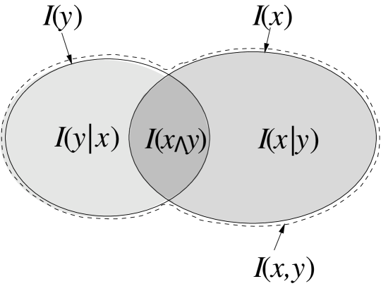
Figure 1: For two correlated events $x$ and $y$, the relations between the information $I(x)$, conditional information $I(x|y)$, joint information $I(x,y)$, and mutual information $I(x\wedge y)$ are illustrated in this diagram.

A bijective mapping between input and output ($x$ completely determines $y$ and vice versa) is achieved if $I(x\wedge y)=I(y)=I(x)$. Note that $I(x\wedge y)\leq\max(I_{x},I_{y})$ – if the space of possible states shrinks when applying $y=f(x)$, there can be at most an injective mapping ($x$ completely determines $y$, but not vice versa).

We first discuss $I(y)$, then the conditional information $I(y|x)$, and consider what processes influence them. We then develop a formalism to derive analytic results for functions that are smooth on scales comparable to the resolution, e.g., if $y$ is the result of applying the logistic map $f(x)=ax(1-x)$ iteratively for a small number of times. The results for long times are discussed later using a different approach.

II.1 Total information: Global phase space considerations

Under any mapping, an ensemble of input values drawn from a given probability distribution is generally mapped onto an ensemble of outputs that is described by another distribution. It is necessary to check whether one or the other requires more information to describe an associated event (a distinct value of input or output).

Sampling a continuous random variable many times with resolution $1/r$ is equivalent to generating a histogram with bins of width $r$. It is useful to separate the information needed to select an element from this histogram into two contributions: one from treating the function underlying the probability distribution as continuous in $x$, and another from the act of separating the input space into $r$ bins. Let us say that we have a probability density $p_{x}(x)$ living on $x\in[0,1]$. The information of this distribution, according to the usual definition Shannon (1948), is

$$I_{c}=-\int dx\;p_{x}(x)\;\log_{2}p_{x}(x).$$ (3)

The discrete probability distribution of the histogram is $P_{x}(x_{i})\approx p_{x}(i/r)/r$. The information of events drawn from this discrete distribution is

$$I_{d}=-\sum_{i}P_{x}(x_{i})\log_{2}P_{x}(x_{i})\approx-\int dx\;r\;(p_{x}(x)/r)\log_{2}(p_{x}/r)=I_{c}+\log_{2}r.$$ (4)

Replacing the sum by the integral is valid as long as $p_{x}(x)$ is reasonably smooth over the range of one bin (which is only roughly valid for the distributions that we discuss in Sec. III.2).

If the input is drawn from a known probability distribution $p_{x}(x)$, the output $y$ follows a probability distribution $p_{y}(y)$ that can be calculated using the rules for transforming probability distributions van Kampen (1992),

$$|p_{x}(x)dx|=|p_{y}(y(x))dy|,\Rightarrow p_{y}(y)=\sum_{\alpha}p(x_{\alpha}(y))\left|\frac{dx}{dy}\right|,$$ (5)

the sum being over all $x$ which map onto $y$. Under all one-dimensional chaotic maps, including the logistic map, two or more input values are mapped onto the same output, a property known as folding.

II.2 Conditional information: Local expansion and shrinkage of phase space

We now study the conditional information $I(y|x)$. While the last section dealt with global properties of the map, here we are averaging over a local property – given some $x_{i}$, we ask, “how much can we know about the output?”, which is independent of the behavior of the map for other input values $x_{k}$.

Let us denote the local conditional information as

$$I_{l}(y|x_{i})=\sum_{j}P_{y|x}(y_{j}|x_{i})\log_{2}P_{y|x}(y_{j}|x_{i}).$$ (6)

As long as bins are small compared to changes in $dy/dx$, trajectories starting from points in the interval $[x_{i},x_{i}+1/r]$ are uniformly distributed over an interval $[y_{x},y_{x}+d/r]$, where $d=|dy/dx|$. The uncertainty about the outcome is determined by the overlap of this interval with the bins (as sketched in Fig. (2)). To account for this, we average over the offset $o\in[0,1]$ which specifies where $y_{x}$ is within a bin.

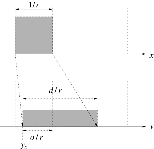
Figure 2: Assuming small bins, trajectories from within one bin in $x$ are mapped uniformly onto one or more bins in $y$.

If a percentage $o$ of a bin is covered with trajectories, the contribution of that bin to the sum in Eq. (6) is given by $I_{p}(o)=-(o/d)\log_{2}(o/d)$. Let us look first at the case $0<d<1$. In that case, either the covered interval is entirely within one bin (if $o>d$) – then the conditional information is $0$ – or the trajectories are split between two bins, resulting in a non-vanishing conditional information. Averaging over $o$ gives

$$\langle I_{l}(y|x)\rangle_{o}=\int_{0}^{d}\left(I_{p}(o)+I_{p}(d-o)\right)\,do+\int_{d}^{1}0\;do=\frac{d}{2\ln 2}.$$ (7)

If $1\leq d<2$, trajectories can be spread out over two or three bins, depending on the offset:

$$I(y|x)=\left\{\begin{array}[]{ll}I_{p}(o)+I_{p}(d-o)&\mbox{~{}~{}~{}for~{}~{}~{}}o>d-1\\ I_{p}(o)+I_{p}(1)+I_{p}(d-1-o)&\mbox{~{}~{}~{}for~{}~{}~{}}o\leq d-1\end{array}\right..$$ (8)

Averaging yields

$$\langle I_{l}(y|x)\rangle_{o}=\log_{2}d+\frac{1}{2d\ln 2}.$$ (9)

Equation (9) thus has two contributions: a term logarithmic in $d$ to account for the bins that are fully covered, and a term from the two partially covered bins, whose impact decays as $1/d$. One can show that Eq. (9) is valid for any value of $d>1$.

To find the average conditional information $I(y|x)$, we can now sum over $x$, with $d(x)=|dy/dx|$:

$$I(y|x)\approx\int\langle I_{l}(y|x)\rangle_{o}dx.$$ (10)

II.3 Folding

It is well known that chaotic iterative maps require a folding mechanism to compensate for stretching of phase space. E.g., in the case of the logistic map, the two branches of the parabola map two input points onto the same output. Clearly, through this process, information about the original state is lost. In the framework presented so far, this is not accounted for explicitly; however, it is contained implicitly in the conditional information. For example, when comparing the identity function $f(x)=x$ with the shift map $f(x)=2x\bmod 1$ (which is chaotic and has folding), both map the unit interval uniformly onto itself and thus have the same global information $I(y)$. However, the latter has a larger average local slope and thus, according to Eq. (9), a larger conditional information, leading to a smaller mutual information between input and output. In this case, the uncertainty in prediction generated through stretching is the same as that in postdiction through folding: going forward in time, one does not know in which of two adjacent bins the output will be, whereas looking back, one has two possible input bins that are well separated, one with $x<1/2$ and one with $x>1/2$.

III Application to the Logistic Map

III.1 Basics of the Logistic Map

We briefly review fundamental properties of the logistic map $f(x)=ax(1-x)$ when used as an iteration (i.e. $x_{t+1}=f(x_{t})$). For $a\leq 1$, there is one (stable) fixed point, namely $x_{t}=0$. Between $1<a<3$, the only stable fixed point is $x_{t}=1-1/a$. At $a=3$, this becomes unstable and gives way to a stable 2-cycle. What follows is a succession of bifurcations ($n$-cycles split into $2n$-cycles) at $a\approx 3.4493$, $3.54396$, $3.56438$ etc., until the cycles merge into a continuous chaotic attractor at $a_{c}\approx 3.569946$ (see also the bifurcation diagram at the top of Fig. 12). The chaotic regime is interrupted by smaller and larger windows of periodic behavior. At $a=4$ one gets what is often referred to as “fully developed chaos;” there, the chaotic attractor spans the interval $[0,1]$.

The Lyapunov exponent, which determines whether two trajectories starting from nearby initial conditions converge or separate exponentially Eckmann and Ruelle (1985), is negative in the fixed point and bifurcation regime, becomes zero at the bifurcation points, and is positive in the chaotic regime.

We now apply the formalism developed in Secs. II.1 and II.2 to the first few iterates of the logistic map $f(x)=ax(1-x)$, then explain the long-time behavior, and give numerical results on intermediate times.

III.2 Short time behavior

Let us consider the probability distribution $p_{y}(y)$ of the first iterate, starting from a uniform distribution. There are two symmetric branches of $y(x)$, and Eq. (5) gives

$$p_{y}(y)=\left\{\begin{array}[]{cl}\frac{2}{\sqrt{a}}\frac{1}{\sqrt{a-4y}}&\mbox{~{}~{}~{}~{}for~{}~{}~{}}y<\frac{a}{4}\\ 0&\mbox{~{}~{}~{}~{}for~{}~{}~{}}y\geq\frac{a}{4}\end{array}\right..$$ (11)

The information of this distribution can be evaluated using Eqs. (3,4):

$$I_{c}(y) = -1-1/\ln 2+\log_{2}a<0,$$ (12)

$$I(y) = -1-1/\ln 2+\log_{2}a+\log_{2}r.$$

In contrast, the information of the uniform distribution was $I_{c}(x)=0$ and $I(x)=\log_{2}(r)$, which means that information about the state of the system was lost – $1/\ln 2-1\approx 0.44$ bits for $a=4$, and more for $a<4$.

The conditional information can be derived from integrating Eqs. (7) and (9) over the input space. In the first iterate of the logistic map, the derivative is smaller than $1$ for $x\in[(1-1/a)/2,(1+1/a)/2]$, and larger in the rest of the domain. Choosing boundaries appropriately and making use of the symmetry of the system, we obtain

$$\int_{0}^{1}P(x)I_{l}(y|x)dx=\frac{a}{4\ln 2}$$ (13)

for $a<1$, and

$$\int_{0}^{1}P(x)I_{l}(y|x)dx = \frac{1}{a\ln 2}\left[\int_{1}^{a}\left(\ln x+\frac{1}{2x}\right)dx+\int_{0}^{1}\frac{x}{2}dx\right]$$ (14)

$$= \frac{1}{a\ln 2}\left[(a+1/2)\ln a+\frac{5}{4}-a\right]$$

for $a\geq 1$. This agrees well with numerical results for finite resolution, as seen in Fig. 3. It should be pointed out that $I(y|x)$ does not explicitly depend on the resolution, in contrast to $I(y)$.

In Fig. 3, $I(y|x)$ represents the uncertainty generated by stretching and compressing; $I(x)-I(y)$ represents the uncertainty through shrinking of phase space; and $I(x)-I(y\wedge x)$ is the average information necessary to reconstruct $x$ from knowledge of $y$. The mutual information $I(y\wedge x)$ is the amount of information about the initial state retained after the mapping.

The mutual information can be calculated by numerical integration over Eq. (9) for the second and third iteration of the logistic map, and good agreement with simulations is found, as shown in Fig. 4. For higher iterates, numerical integration becomes difficult. Numerical integration over the probability distribution of outputs also becomes less accurate, and the approximation made in Eq. (4) becomes visibly wrong for resolutions as coarse as $r=100$.

While Figs. 3 and 4 do not show a clear distinction between the fixed point/cyclic regime and the chaotic regime, one can see that conditional information (i.e., uncertainty generated by the dynamics) increases with $a$, whereas $I(y)$ develops dips. For example, the dip at $a\approx 2$ represents rapid convergence to the fixed point far from the bifurcation points $a=1$ and $a=3$. Correspondingly, $I(y\wedge x)$ is no longer monotonic in $a$ – several maxima of conserved information emerge.

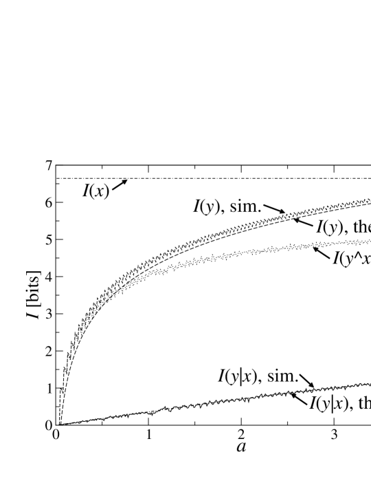
Figure 3: Conditional, mutual and total information of input and output for $r=100$ for one time step, compared to Eqs. (III.2) and (14).

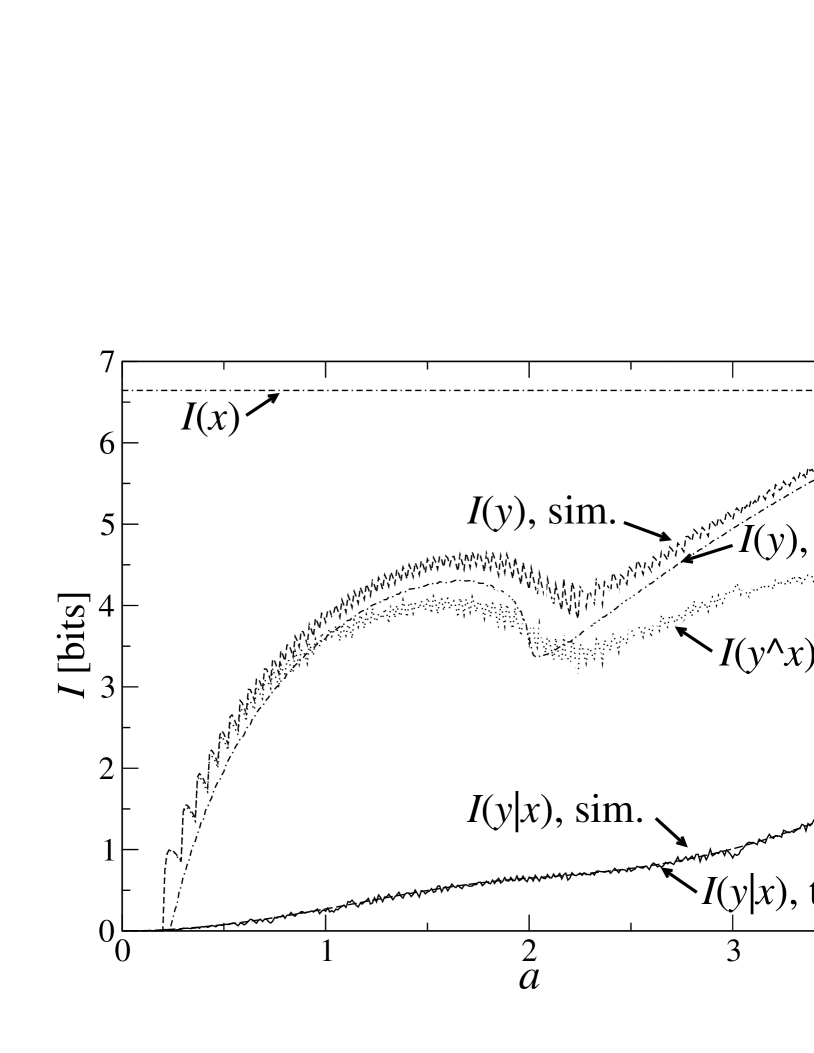
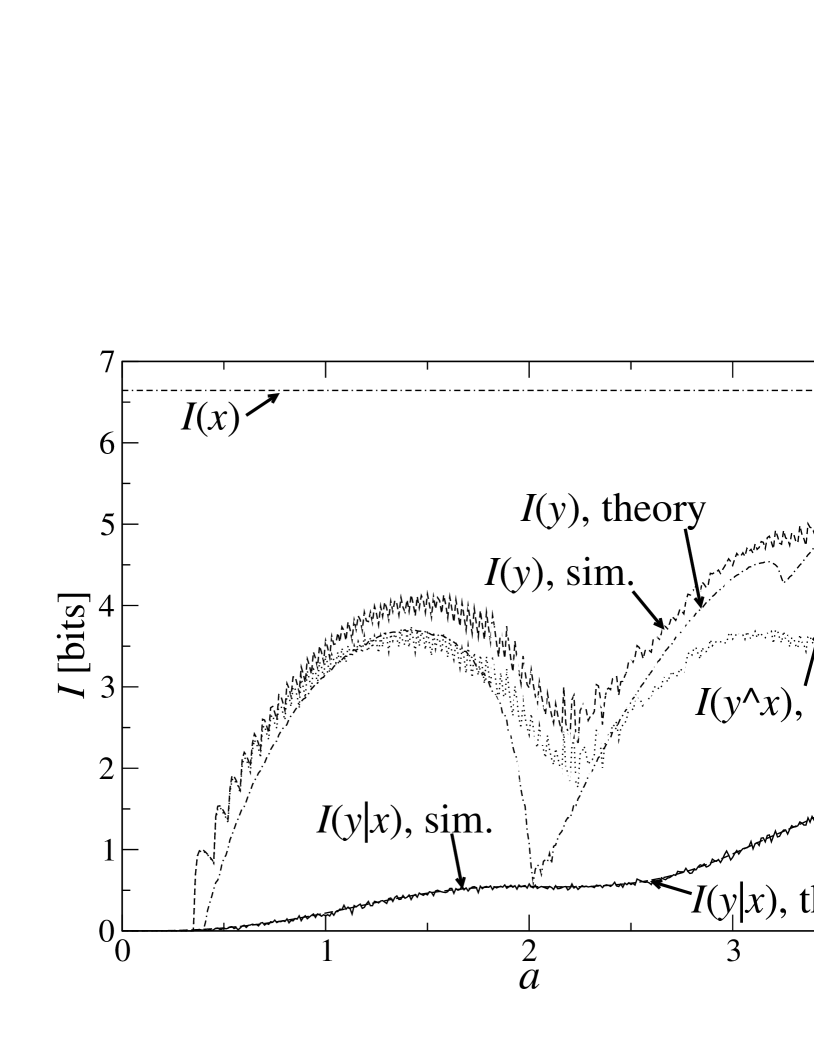
Figure 4: Conditional, mutual and total information of input and output for $r=100$ for two and three time steps, compared to results of numerical integration. $I(y|x)$ does not depend strongly on $r$, whereas the other quantities include an additive term of $\log_{2}r$.

III.3 Long-time behavior

For very long times, some simple statements about the information in the output can be made: if the map has a single fixed point ($0<a<3$), $I(y)=0$. For a cycle of length $2^{n}$, $y(t)$ can be defined completely by stating what branch of the cycle it is on; the information is therefore $n$ bits if the resolution is fine enough to resolve each branch of the cycle, and each branch has an equally large basin of attraction, and smaller otherwise. In the chaotic regime, there is a probability distribution filling a finite fraction of the interval $[0,1]$ for most values of $a$, and cycles of various lengths in certain periodic windows. The continuous information $I_{c}$ will therefore be less than one, and the information at finite resolution less than or equal to $\log_{2}r$, with visible dips in the periodic windows. Numerical results of $I(y)$ for $r=100$ and $r=10000$ shown in Fig. 5 demonstrate these features.

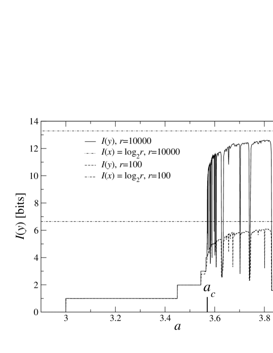
Figure 5: Information $I(y)$ of the output distribution for $r=100$ and $r=10000$, for $t\rightarrow\infty$, compared to the input information $I(x)$.

The mutual information is at most as large as the total information, therefore it will be $0$ as well for $a<3$. In the bifurcation regime, dynamics are fairly predictable. The basins of attraction for each branch of the cycle are fractals, reminiscent of Cantor sets, as shown in Fig. 6. If the bins are small enough such that most bins map exclusively to one branch of a $2^{n}$-cycle, the mutual information is of order $n$ bits.

In the chaotic regime, information about the original state is lost at a rate approximately equal to the Lyapunov exponent Shaw (1981); Pompe et al. (1986), which here is between 0 and 1; we therefore expect mutual information to be $0$ after $\mathcal{O}(\log r)$ time steps. Note that this affects prediction as well as postdiction: even though $I(y)$ is not much smaller than $I(x)$ for $a=4$, in the absence of mutual information, it is as impossible to tell where the system came from as where is is going.

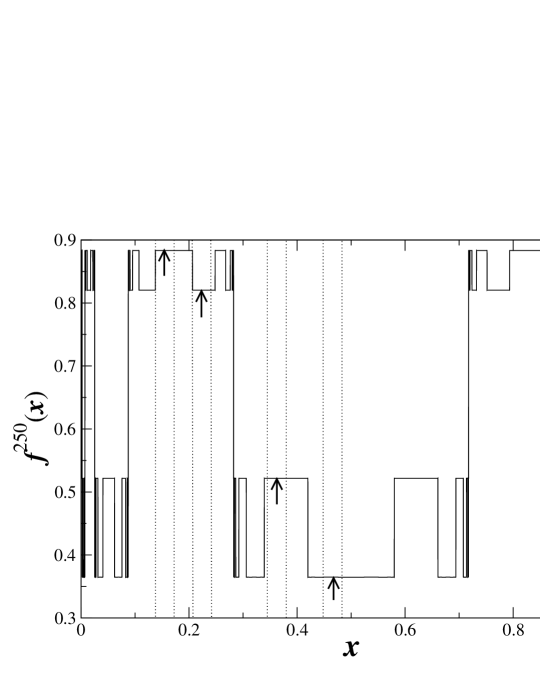
Figure 6: The 250th iterate of the logistic map at $a=3.54$, as an example of the long-time dynamics. The dominant values are the branches of the 4-cycle; one sees the fractal structure of the basins of attraction of each branch. Iterates at times $250+4n$ look indistinguishable. The dotted lines indicate input bins at a resolution of $r=29$ that map uniquely onto one branch of the cycle (see Sec. IV).

III.4 Intermediate times

Figure 7 shows the mutual information for $r=1000$ at various intermediate times $t$, measured by scanning input space with a step width small compared to the bin width. Apart from the long-time features explained in Sec. III.3, one notices several peaks. The narrow peaks (e.g. near $a=2.5$) occur when the fixed point is very close to the boundary between two bins, such that small deviations from the fixed point lead to ambiguities in the outcome. They change position if the binning is chosen differently.

The wider peaks at $a=1$, $3$, and $3.54$ correspond to the bifurcation points. There, the Lyapunov exponent is 0; deviations from the fixed point or cycle decay like a power law rather than exponentially. In the chaotic regime, the mutual information quickly drops to $0$, apart from peaks that correspond to periodic windows (e.g. at $a\approx 3.83$).

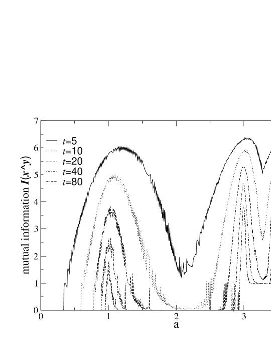
Figure 7: Mutual information between input and output for different numbers of iterations $t$, for a resolution $r=1000$. For smaller resolutions, curves look similar, but more jagged. Also, the maximum of the curves has an additive term of $\log_{2}r$.

IV Communication through a logistic map channel

We now interpret and expand the results of previous sections with a view to the problem of communication in the following scenario: a sender A wants to transmit a message to a receiver B by setting the initial state of the logistic map with some finite resolution. B receives the state after $t$ iterations of the logistic map and interprets it. For what values of $a$ and $t$ can A expect any degree of transmission, and what resolution do A and B need?

The scenario may seem contrived; however, setting the initial state of some physical system (like a sheet of paper, or a hard disk) in the hope that someone will be able to read it is the usual way of transmitting messages over long times. Usually people choose systems whose dynamics are somewhat stable to perturbations and slow compared to the time $t$, but they may not always have that choice. Let us look at two different communication problems.

IV.1 Reconstructing the initial state

In this scenario, A wants B to know the state that A started the system in. The problem is then essentially one of postdiction for the recipient, and the relevant quantity is the difference between the mutual information $I(y\wedge x)$ and the input information $I(x)$. Surprisingly, for very short times, Figs. 3 and 4 show that B has the best chances of postdicting the initial state in the chaotic regime near $a=4$ – the loss of information through chaos is not as significant as that through phase space shrinking in the low-$a$-regime. Note that at least one bit is lost: since $f(x)$ is symmetric around $x=1/2$, it is impossible to tell whether the system was started on the left or right branch.

For intermediate times, at high $a$, chaotic dynamics eliminates all information about the initial state; so does fast convergence to a single fixed point for small $a$. As Fig. 7 shows, B’s situation is best if $a$ is close to one of the bifurcation points, where convergence follows a power law rather than an exponential.

In the limit of very long times, when the system has converged to its attractor, the only regime where information about the initial state persists is the bifurcation regime. What value of $a$ gives optimal transmission depends on the resolution: the recipient has to be able to resolve all branches of the cycle to make full use of the remaining information.

In all three time regimes, it is important for the recipient to know the precise time at which the system was initialized. The information required to specify the time lag has to be included in the conditional information $I(x|y)$. To give a simple example: in the long-time regime, if the time is either $t$ or $t+1$ with probability $1/2$, an additional bit of information is required to reconstruct the initial state.

IV.2 Determining the final state with certainty

The second communication problem is this: A only wants to send B a message that B can decode with certainty: A chooses the initial state (again with resolution $r$) such that all trajectories from that state end in one output bin. The relevant questions are now, what resolution do A and B need to specify at least two different final states for various times and amplifications; and, given a certain resolution, how many distinct final states exist that can be achieved with certainty by choosing an appropriate initial state? This is a problem of prediction on the part of the sender.

The answer is clearest for long times: as described above, the only regime where information persists and communication is possible at all is that of cyclic behavior. The sender needs to identify input bins that lie completely in the basin of attraction of one branch of the cycle, such that each initial value in the bin leads to the same final value. One such bin should be found for each distinct branch, and the resolution must be sufficient for the recipient to identify each branch (see Fig. 6 for an example of such a set of bins). Numerics show that the latter constraint is weaker than the first: it is the sender’s resolution that limits communication. We find that a resolution of 7 bins is sufficient for the 2-cycle at values of $a=3.5$; thus, $\log_{2}7\approx 2.8$ bits are needed to specify the input to transfer one bit to the recipient. For longer cycles, the ratio can be more efficient: 29 bins are enough to resolve the 4-cycle at $a=3.54$, yielding $4.86$ bits of input for 2 bits of output. At $a=3.562$, a resolution of 122 specifies each branch of the 8-cycle, giving 3 bits of output for $6.93$ bits of input. (We assume that $a$ is constant and precisely known to the sender and recipient.)

In the short and intermediate time regimes, the number of distinct final states that can be reached with certainty increases roughly linearly with resolution. The slope is a function of both $t$ and $a$, and its value indicates the amount of information lost in the channel. Fig. 8 shows the number of distinct states at $r=1000$ for different times and amplifications. Some features are similar to Fig. 7: for longer times, peaks at the bifurcation points emerge, representing the slow loss of information. Between the bifurcation points, plateaus at values of 2 and 4 can be seen for $t=40$. In the chaotic regime, the number of predictable final states goes to zero with increasing time.

The most surprising feature of Fig. 8 is that the curve for $t=1$ is not monotonic, and even drops below those for longer times. The reason is that the first iterate has a slope greater than $1$ for most $x$ values at high $a$, which makes unique prediction impossible. Further iterations can re-compress parts of the state space that were stretched in the first iteration, leading to a better match between input and output bins.

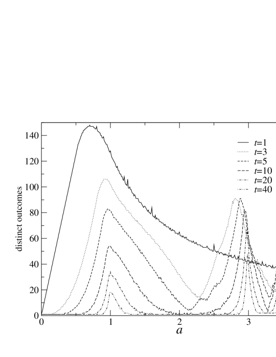
Figure 8: The number of distinct final states that can be reached with certainty by choosing an appropriate initial state. Both sender and recipient use $r=1000$.

V Scale-resolving representations of real numbers

Dissipation and chaos have a common aspect: in both cases the dynamics makes a connection between large and small scales. Chaotic dynamics amplify small differences in the initial states until they reach macroscopic proportions, whereas dissipative dynamics shrink differences until they vanish below the threshold of perception. To represent this adequately, we first have to make clear what we mean by information on different scales.

Let us consider real numbers $x$. On one hand, each real number can be represented by one point on the real axis – it is a one-dimensional quantity. On the other hand, in the usual descriptions (decimal, binary etc.), real numbers are represented by a set of integers that stand for different scales – the scales of 1s, 10s, 100s, etc. This makes sense because it reflects what happens when some $\Delta x$ is added to $x$: the digits of $x$ are strongly affected for all scales finer than the scale of $\Delta x$, and weakly affected for coarser scales.

There are two problems with the usual representations: first, they are discontinuous: a small change on a fine scale will have no effect at all on coarser scales most of the time, but a dramatic effect in rare cases (such as when $0.001$ is added to $0.999$). This is a necessary side effect of using discrete (integer) representations on each scale. Second, they do not lend themselves to simple modification under multiplication: multiplication is basically a convolution of the representations of the two factors. Whereas multiplications with numbers that have a simple representation in the chosen base gives a shift (e.g. multiplication with 10 in the decimal representation just shifts the decimal point), all other factors lead to changes throughout the scales. It may therefore be worthwhile to think about alternative representations for which the information content of various scales is easy to visualize.

First, we need to decide what properties we expect the representation to have. At a very basic level, each real number should map onto one representation, and each representation should map onto at most one real number. (Since we want to include the option of representing one real number by a set of real or complex numbers, a bijective mapping is not generally possible.) Also, elements of the representation corresponding to finer scales should not include the information at coarser scales – otherwise they would not be specific to their scale. One way of achieving this is using periodic functions, with the period equal to the scale to be studied.

V.1 The Clockwork Representation

Using the most natural periodic function, one obtains what we call the clockwork representation (CR). It maps each real number $x$ onto set of complex numbers

$$c_{j}(x)=\exp(2\pi i\;2^{j}x),$$ (15)

with $j$ identifying the scale. The base $2$ is was chosen in analogy to the familiar binary representation – any number other than 1 can also be used. The term “clockwork representation” was chosen because each digit can be thought of as a cog in a clockwork of consecutively smaller cogs, as depicted in Fig. 9 – two turns of $c_{2}$ cause one turn of $c_{1}$, but four turns of $c_{3}$. Using a different base is equivalent to using cogs of a different radius ratio.

We can use the usual laws for exponential functions to see how addition and multiplication of numbers carries over to their clockwork representation:

$$c_{j}(x+y) = \exp(2\pi i\;2^{j}x)\exp(2\pi i\;2^{j}y)=c_{j}(x)\,c_{j}(y);$$ (16)

$$c_{j}(ax) = \exp(2\pi i\;2^{j+\log_{2}a}x)=c_{j+\log_{2}a}x.$$ (17)

The second line appears a little problematic for two reasons: first, it introduces an asymmetry between the object under consideration $x$ and the factor $a$ – the result might as well have been written as $c_{j+\log_{2}x}a$. This is, in some cases, desired: there is often a conceptual difference between the dynamical variables and the parameters of a model. Second, scales become continuous rather than discrete. However, this is more of an advantage rather than a disadvantage. The outcome is well-defined even for non-integer scales, as opposed to the case of discrete representations: one can write a number in base 2 or base 3, but not base $2.5$.

The CR gives a set of complex numbers; while it is clear how to do mathematical operations on them, it is not completely obvious how to display them. It can be argued that usually one is interested in the imaginary part: it gives $0$ for scales much coarser than that of the number under consideration, and it gives $0$ for fine scales if $x$ is a power of $2$, much like the bits in a binary representation would.

Figure 9: The clockwork representation; each digit represents one cog.

Another way to think about the CR is to look at the continuous function that generates the digits, as in Fig. 10: it shows $\sin(2\pi 2^{j})$, which is the imaginary part of the CR of the number $1$. It has an exponential tail toward coarse scales and an oscillating part with a frequency that increases exponentially toward fine scales. The CR picks out the values of this function at integer values of $j$. For any other number $x$, shift the curve to the left by $\log_{2}x$, and again pick the values at integer values of $j$.

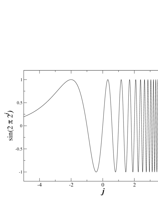
Figure 10: The clockwork representation of the number 1: each digit corresponds to the value of this function at integer values of $j$.

V.2 Using the CR in the logistic map

As explained in the previous sections, the clockwork representation can give an impression about how numbers change on different scales of resolution. This can be applied to illustrate the behavior of the logistic map. The most obvious case is that of convergence to a fixed point or cycle, as shown in Fig. 11: for $a=2.95$ (slightly below the first period doubling), a random initial state (left side) converges to the fixed point (right side); differences from the final state occur on finer and finer scales as time progresses, resulting in a ridge traveling to finer scales.

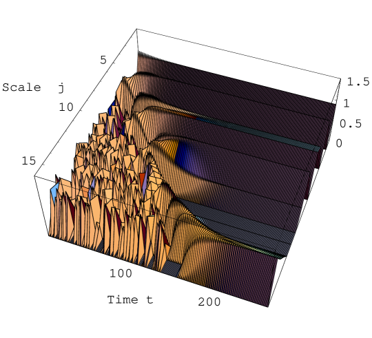
Figure 11: Imaginary part of the CR of the $t$th iterate of the logistic map, at $a=2.95$. Deviations from the fixed point travel “downstream,” to finer scales.

This ridge also shows up in a two-dimensional Fourier transform of the CR, seen in Figs. 12: for $a=2.8$, the absolute squared Fourier transform of the CR shows diagonal ridges. To make the effect clearer, the plot averaged over 100 uniformly distributed initial conditions. For $a=3.05$, one sees a horizontal stripe in the center of the figure in addition to the diagonal structures, indicating that the final state has a period of 2.

The slope of the diagonal structures during convergence to a limit cycle is directly proportional to the Lyapunov exponent $\lambda$: during each time step, the deviation from the limit cycle diminishes by a factor of $\exp{\lambda}$. In a plot of $\log_{2}x$ vs. $t$ such as Fig.11, the ridge therefore has a slope of $\lambda/\ln 2$. In a Fourier transform plotted as frequency vs. inverse scale, the ridge causes diagonal structures of the same slope. To illustrate this, dashed lines of slope $\lambda/\ln 2$ are shown in Fig. 12.

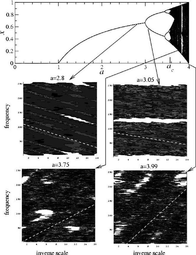
Figure 12: Squared amplitude of the Fourier transform of the CR, averaged over more than $100$ initial conditions, at $a=2.8$, $3.05$, $3.7$, and $4.0$. Dashed lines indicate a slope $\lambda/\ln 2$, where $\lambda$ is the Lyapunov exponent.

It is not obvious that this holds for the chaotic regime as well: there, $x$ keeps changing on all scales, not just increasingly small ones, and multiplication induces a folding of small and large scales. Interestingly, however, similar structures can be found in the chaotic regime as well: even though a 3D plot of the CR versus time looks unstructured and chaotic, a Fourier transform averaged over sufficiently many initial conditions often reveals diagonal stripes (Fig. 12, bottom), this time tilted in the opposite way – which indicates information traveling to coarser scales rather than finer ones. Although the structures are less clear than for convergence, an approximate correspondence between the slope of the structures and the Lyapunov exponent still holds for many values of $a$, as shown by the diagonal lines in the plots. In other cases, the structures are less clear: in particular, for $a=4.0$ the plot shows strong diagonal structures with a slope of 2 overlaid on a weak diagonal with a slope of approximately $1$. The latter is expected from the value of the Lyapunov exponent.

It should be noted that using the binary representation instead of the CR yield similar pictures (albeit more noisy) for the convergence to a fixed point, but shows no discernible structures for the convergence to the chaotic attractor.

VI Summary

We have presented a study of the loss of information through the nonlinear dynamics of the logistic map, using analytical means for short times and numerics and heuristic arguments for long times. As Secs. II and IV have shown, different processes are relevant in the different regimes: in the small-$a$ regime, shrinking phase space quickly makes postdiction impossible and prediction trivial, thus eliminating the possibility of communication. In the chaotic regime (very high $a$), phase space is largely conserved, but sensitivity to initial conditions prevents both prediction and postdiction for longer times. The bifurcation regime provides a middle ground: some information about the initial state persists, determining what branch of the cycle one finds the system in. The basins of attraction for the branches have a fractal structure, which means that some large intervals of initial values exist that lead to one branch with certainty. At the bifurcation points, convergence to the final state is slow, which makes some transfer of information possible for intermediate times.

The clockwork representation introduced in Sec. V is a continuous generalization of the usual discrete (binary, decimal etc.) representations in which addition and multiplication of two objects are more transparent than in the discrete case, and which allows for a more elegant visualization of the flow of information between scales and the convergence to fixed points. It is even possible to identify the slope of structures in the Fourier transform of the CR with the Lyapunov exponent of the map. While the CR thus seems to be a conceptual and visual tool of some use, it remains to be seen whether this representation will find additional applications in analyzing dynamical systems.