The analytic structure of 2D Euler flow at short times

Abstract

Using a very high precision spectral calculation applied to the incompressible and inviscid flow with initial condition $\psi_{0}(x_{1},\,x_{2})=\cos x_{1}+\cos 2x_{2}$, we find that the width $\delta(t)$ of its analyticity strip follows a $\ln(1/t)$ law at short times over eight decades. The asymptotic equation governing the structure of spatial complex-space singularities at short times (Frisch, Matsumoto and Bec 2003, J. Stat. Phys. 113, 761–781) is solved by a high-precision expansion method. Strong numerical evidence is obtained that singularities have infinite vorticity and lie on a complex manifold which is constructed explicitly as an envelope of analyticity disks.

Fluid Dyn. Res. 36, 221–237 (2005).

1 Introduction

In early September 2001 one of the authors (UF) attended the Zakopane meeting on Tubes, Sheets and Singularities (Bajer and Moffat, 2003) which was also attended by Richard Pelz. There were many discussions about the issue of finite-time blowup for 3D incompressible Euler flow. Richard, who had studied a flow introduced by Kida (1985), had evidence in favor of blowup but one could not rule out that the highly special structure of this flow would lead to quasi-singular intermediate asymptotics. The three authors of this paper then decided to embark in a long-term project aimed at getting strong evidence for or against blowup for a wide class of flows encompassing the Taylor–Green flow (Brachet et al., 1983) and the Kida–Pelz vortex (Kida, 1985; Pelz, 1997; Pelz and Gulak, 1997; Pelz, 2001), namely space-periodic flow with or without symmetry having initially only a few Fourier harmonics. Such initial flow is not only analytic but also entire: there is no singularity at finite distance in the whole complex spatial domain.

As has been known since the mathematical work of Bardos, Benachour and Zerner (1976), any real finite-time singularity is preceded by complex-space singularities approaching the real domain and which can be detected and traced using Fourier methods (Sulem, Sulem and Frisch, 1983; Frisch, Matsumoto and Bec, 2003). This method is traditionally carried out by spectral simulations which run out of steam when the distance $\delta(t)$ from the real domain to the nearest complex-space singularity is about two meshes. We pointed out in a recent paper (Frisch, Matsumoto and Bec, 2003, henceforth referred to as FMB), which also reviews the issue of blowup, that it may be possible to extend the method of tracing of complex singularities by performing a holomorphic transformation mapping singularities away from the real domain and, perhaps doing this recursively. This is the basic idea of the spectral adaptive method which aims at combining the extreme accuracy of spectral methods with the local mesh refinement permitted by adaptive methods.

In one dimension the complex-space singularities of PDE’s are isolated points, at least in the simplest cases, as for the Burgers equation. In higher dimension they are extended objects, such as complex manifolds. Understanding the nature and the geometry of such singularities is a prerequisite for mapping them away. Many aspects can already be investigated in the two-dimensional case for which we know not only that blowup is ruled out, but we also know that the flow stays a lot more regular than predicted by rigorous lower bounds (basically $\delta(t)$ seems to decrease exponentially whereas the bound is a double exponential in time). In FMB we gave some evidence that in 2D the complex singularities are on a smooth manifold, but the nature of the singularities was not very clear and in particular the issue of finiteness vs. blowup of the complex vorticity was moot.

In FMB we also pointed out that the issue of singularities can be simplified if we limit ourselves to short times. Let us briefly recall the setting. We start with the 2-D Euler equation written in stream function formulation

$$\partial_{t}\nabla^{2}\psi=J(\psi,\nabla^{2}\psi),$$ (1)

where $J(f,g)\equiv\partial_{1}f\partial_{2}g-\partial_{1}g\partial_{2}f$. As in FMB, we focus on the two-mode initial condition

$$\psi_{0}({\bm{x}})=\cos(x_{1})+\cos(2x_{2}),$$ (2)

one of the simplest initial condition having nontrivial Eulerian dynamics. The solution $\psi({\bm{z}},t)$, obtained by analytic continuation to complex locations ${\bm{z}}={\bm{x}}+i{\bm{y}}$, is expected to have singularities at large imaginary values when $t$ is small. If one focuses on the quadrant $y_{1}\to+\infty$ and $y_{2}\to+\infty$, an asymptotic argument given in FMB suggests looking at solutions satisfying the similarity ansatz

$$\psi({\bm{z}},t) = (1/t)F(\tilde{\bm{z}}),$$ (3)

$$\tilde{\bm{z}} = (\tilde{z}_{1},\,\tilde{z}_{2})\equiv(z_{1}+i\ln t,\,z_{2}+(i/2)\ln t).$$ (4)

Substitution in (1) gives the similarity equation

$$\tilde{\nabla}^{2}(-1+i\tilde{\partial}_{1}+(i/2)\tilde{\partial}_{2})F=\tilde{J}(F,\tilde{\nabla}^{2}F),$$ (5)

where the overscript tilde means that the partial derivatives are taken with respect to the new variables. The initial condition (2) becomes a boundary condition

$$F(\tilde{\bm{z}})\simeq\frac{1}{2}\left({\rm e}^{-i\tilde{z}_{1}}+{\rm e}^{-2i\tilde{z}_{2}}\right),\quad\tilde{y}_{1}\to-\infty,\,\,\,\,\tilde{y}_{2}\to-\infty.$$ (6)

Note that (5) has no time variable. Its solution can be shown to be analytic for sufficiently negative $\tilde{y}_{1}$ and $\tilde{y}_{2}$. If it has singularities in the real or complex domain then, by (4), the solution of the original Euler equation should have short-time singularities at a distance $\delta(t)\propto\ln(1/t)$.

The outline of the present paper is as follows. In Section 2 we check the logarithmic law for $\delta(t)$ and thus the validity of the similarity ansatz. In Section 3 we develop a new technique for solving the similarity equation (5) in both the real and complex domains. In Section 4 we present numerical results on the nature and the geometry of the singularities. In Section 5 we show how to actually construct the singular manifold from the Fourier transform of the solution. In Section 6 we make some concluding remarks.

2 Numerical validation of the short-time behavior

The standard way of measuring the distance $\delta$ of the nearest complex-space singularity (also called the width of the analyticity strip) is to use the method of tracing (Sulem, Sulem and Frisch, 1983). Indeed, the spatial Fourier transform $\hat{v}_{{\bm{k}}}$ of a periodic function $v({\bm{x}})$ has its modulus decreasing at large wavenumbers $k\equiv|{\bm{k}}|$ as $e^{-\delta k}$ in both one and several space dimensions. More precisely, for each direction $\hat{\bm{k}}\equiv{\bm{k}}/k$, the modulus of the Fourier transform decreases as $e^{-\delta_{\hat{\bm{k}}}k}$; the width of the analyticity strip is then the minimum over all directions $\hat{\bm{k}}$ of $\delta_{\hat{\bm{k}}}$ which – by a steepest descent argument – also controls the high-$k$ decrease of the angle average of the modulus of the Fourier transform.

Accurate measurement of the width of the analyticity strip $\delta$ gets difficult when it becomes smaller than a few meshes, so that there is not enough resolution to see long exponential tails (Brachet et al., 1983). A different difficulty appears when $\delta$ is very large and the Fourier transform decreases so rapidly that it gets lost in roundoff noise at rather small $k$’s. To check on the logarithmic law of variation of $\delta(t)$ at short times for the full time-dependent Euler equation (1), we have to face the latter difficulty. To overcome it, we employed a 90-digit multiprecision spectral calculation with the number of grid points ranging from $64^{2}$ to $128^{2}$ The temporal scheme is fourth order Runge-Kutta. Fig. 1 shows the $k$ dependence at various short times of the angular averages of the modulus of the Fourier transform of the velocity ${\bm{v}}\equiv(\partial_{2}\psi,\,-\partial_{1}\psi)$, where $\partial_{1}$ and $\partial_{2}$ are the derivatives with respect to $x_{1}$ and $x_{2}$. Note that there is a strong odd-even wavenumber oscillation. This has to do with the interference of two complex singularities separated by $\pi$ in the $x_{2}$ direction (a consequence of a symmetry of the initial condition).

Figure 1: Angular averages of the modulus of the velocity Fourier modes at short times calculated with 90-digit precision. Strong oscillations between odd and even $k$’s are due to the symmetry of the initial condition (2). The values of the time steps for integrating the Euler equation with $64^{2}$ and $128^{2}$ grid points are respectively $2\times 10^{-11}$ and $5\times 10^{-6}$.

A very clean exponential decrease is observed for even wavenumbers. This allows the measurement of $\delta(t)$ for hundreds of values of $t$ covering a very wide range, as shown in Fig. 2 in log-lin coordinates.

Figure 2: Width of the analyticity strip $\delta(t)$ at short times $2\times 10^{-10}\leq t\leq 7.3\times 10^{-1}$ measured from the angular average of the modulus of the velocity Fourier modes restricted to even $k$’s.

It is seen that, up to approximately $t=10^{-2}$, the logarithmic law is satisfied over eight decades, a range which could not be achieved without the use of very high-precision computations.

3 Solving the similarity equation

We are interested in space-periodic solutions to (5) satisfying the boundary condition (6). This problem can be solved exactly using Fourier series

$$F({\bm{z}})=\sum_{k_{1}=-\infty}^{\infty}\sum_{k_{2}=-\infty}^{\infty}\hat{F}_{k_{1},k_{2}}e^{i(k_{1}z_{1}+k_{2}z_{2})}.$$ (7)

Note that we have dropped all tildes on the space variables since from now on we will work exclusively with the similarity variables. Obviously, the boundary condition (6) allows the presence only of Fourier harmonics with wavevectors in the quadrant $(k_{1}\leq 0,\,\,k_{2}\leq 0)$. After (5) is rewritten in terms of the Fourier coefficients of $F$, the multiplications appearing in the Jacobian go over into simple convolutions with only finitely many terms, because all wavevectors involved must have non-positive components. It follows that, for integer $n\geq 1$, all Fourier coefficients for wavevectors which are on the line $2k_{1}+k_{2}=-2(n+1)$ (see Fig. 3)

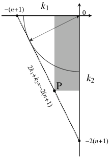
Figure 3: Region in the wavenumber space relevant in calculating the Fourier coefficients $\hat{F}_{k_{1},\,k_{2}}$ on the line $2k_{1}+k_{2}=-2(n+1)$. The largest disk centered at the origin fitting into this region is also shown.

are expressible in terms of the finitely many Fourier coefficients with wavevectors lying above this line. More precisely, for any point P on this line, the region of dependence is the grey-shaded rectangle. Specifically, we define the selective Fourier sum over this line

$$F_{n}({\bm{z}})\equiv\sum_{\sigma=0}^{n+1}\hat{F}_{-\sigma,-2(n+1-\sigma)}e^{-i(\sigma z_{1}+2(n+1-\sigma)z_{2})},$$ (8)

so that

$$F({\bm{z}})=\sum_{n=0}^{\infty}F_{n}({\bm{z}}).$$ (9)

From (5) we then obtain the recursion relations

$$\nabla^{2}F_{n+1}=\frac{1}{n+1}\sum_{r=0}^{n}J(F_{r},\nabla^{2}F_{n-r}),$$ (10)

with

$$F_{0}({\bm{z}})=\frac{1}{2}\left(e^{-iz_{1}}+e^{-2iz_{2}}\right).$$ (11)

Equation (10) can then be rewritten as a set of algebraic equations for the Fourier coefficients:

$$\hat{F}_{k_{1},\,k_{2}} = \sum_{p_{1}=k_{1}}^{0}\sum_{p_{2}=k_{2}}^{0}T_{{\bm{k}}}({\bm{p}})\,\hat{F}_{p_{1},\,p_{2}}\,\hat{F}_{k_{1}-p_{1},\,k_{2}-p_{2}}\,,$$ (12)

$$T_{{\bm{k}}}({\bm{p}}) \equiv \frac{2}{2k_{1}+k_{2}+2}\frac{|{\bm{k}}-{\bm{p}}|^{2}({\bm{p}}\wedge{\bm{k}})}{|{\bm{k}}|^{2}}\,,$$ (13)

where ${\bm{k}}\wedge{\bm{k}}^{\prime}\equiv k_{1}k^{\prime}_{2}-k_{2}k^{\prime}_{1}$. One could solve the Poisson equations (10) which recursively define the $F_{n}$’s using FFT methods as in Brachet et al. (1983). Alternatively – and this is the method used here – equations (12)-(13) can be used to calculate recursively the exact expressions of all the Fourier coefficients. The first two $F_{n}$’s are

$$F_{1}({\bm{z}}) = -\frac{3}{10}e^{-i(z_{1}+2z_{2})},$$ (14)

$$F_{2}({\bm{z}}) = -\frac{3}{340}e^{-i(z_{1}+4z_{2})}+\frac{3}{40}e^{-i(2z_{1}+2z_{2})}.$$ (15)

We have numerically determined the $F_{n}$’s for $n$ up to $n_{\rm max}=1500$, using quadruple-precision (35-digit) accuracy. As we shall see in the next section, lower accuracy would give spurious results. From (12) and (13), the $\hat{F}_{k_{1},\,k_{2}}$ are obviously real. Furthermore, we find numerically that their signs alternate: specifically $(-1)^{k_{1}}\hat{F}_{k_{1},\,k_{2}}\geq 0$, for all $(k_{1},k_{2})$ except $(-1,0)$.

4 Numerical results on singularities

We shall work here mostly with shell-summed (Fourier) amplitudes. For a given periodic function $f$, we define its shell-summed amplitude as

$$A^{(f)}_{K}\equiv\sum_{K\leq|{\bm{k}}|<K+1}|\hat{f}_{\bm{k}}|,$$ (16)

where the $\hat{f}_{\bm{k}}$ are the Fourier coefficients of $f$. The shell-summed amplitudes for the solution $F$ to the similarity equation (5) can be calculated, in principle exactly, for all wavenumbers $K$ such that $K+1<k_{\rm max}$ where $k_{\rm max}=(2/\sqrt{5})(n_{\rm max}+1)$, this being the radius of the largest disk centered at the origin and contained in the triangular region of Fig. 3.

Fig. 4 shows, as a function of $K$, the shell-summed amplitude of $F$ for $n_{\rm max}=1500$. As seen in Fig. 4(a), the results obtained with 15 and 35 digit precisions differ markedly beyond wavenumber 800. Even the 35-digit calculation becomes unreliable beyond wavenumber 1300. In FMB, when we discussed results about singularities without resorting to short-time asymptotics, we reported various difficulties: the need to perform a kind of Krasny filtering (Krasny, 1986; Majda and Bertozzi, 2001; Caflisch, Hou and Lowengrub, 1999) and our failure to improve the range of scaling by going to resolutions higher than $512^{2}$. It is now clear that the key to clean results is to use high precision.

We fit the shell-summed amplitude of $F$ by a function of the form $CK^{-\alpha}\exp(-\delta K)$ and find the best fit to be $0.5K^{-2.16}\exp(-0.0065K)$, as shown in Fig. 4(b). The fit is done by least squares in the lin-log representation over the interval $0\leq K\leq 1100$.

Figure 4: (a) Shell summed amplitudes $A^{(F)}_{K}$ for the stream function $F$ calculated with 15 and 35-digit precisions in lin-log coordinates. The strange behavior of the 15-digit result in the high wavenumber region $k\geq 800$ is due to insufficient precision. (b) Shell summed amplitude $A^{(F)}_{K}$ calculated with 35-digit precision and almost overlapping least square fit to $CK^{-\alpha}\exp(-\delta K)$ in lin-log coordinates. Numerical instability is observed for $K>1300$. Inset: $A^{(F)}_{K}$ with 35-digit precision and its least square fit in log-log coordinates.

Hence, the solution to the similarity equation has complex-space singularities, the closest one being within $\delta\approx 0.0065$. This relatively small value, for an equation in which all the coefficients are order unity, is accidental and can be changed by slightly modifying the coefficients in front of the two harmonics in the initial condition (2) and in (11), as will be shown later in this section.

The angular dependence of the mode amplitude at high wavenumbers can also be obtained. Fig. 5 shows that $|\hat{F}_{\bm{k}}|$ decreases exponentially with $k\equiv|{\bm{k}}|$ for a given direction $\hat{\bm{k}}=(\cos\theta,\,\sin\theta)$. We see that the logarithmic decrement, denoted by $\delta(\theta)$, varies strongly with $\theta$. Its variation is shown in Fig. 6 for $\pi<\theta<3\pi/2$, that is over the third angular quadrant where $k_{1}$ and $k_{2}$ are negative. Obviously, the width of the analyticity strip is

$$\delta=\min_{\theta}\,\delta(\theta),$$ (17)

the minimum being achieved in the most singular direction $\theta=\theta_{\star}$, such that $\tan\theta_{\star}\approx 1.62$. The function $\delta(\theta)$ can be related to the singular manifold (see Section 5).

Figure 5: Amplitudes of the Fourier modes $|\hat{F}_{{\bm{k}}}|$ along five different directions from $1.05\pi$ to $1.32\pi$ (from bottom to top)

Figure 6: Logarithmic decrement $\delta(\theta)$ as a function of the polar angle $\theta$ in the $(k_{1},\,k_{2})$ plane. The minimum of $\delta(\theta)$ is around $0.0065$. The most singular direction is $\theta_{\star}=1.324\pi$.

As in one dimension, the prefactor of the exponential in the shell-averaged amplitude $A_{K}^{(F)}$ contains information about the nature of the singularities. In the inset of Fig. 4 we see about one decade of power-law scaling before the exponential falloff. This range can be increased by moving closer to the singularity, more precisely to the point ${\bm{z}}_{\star}$ on the singular manifold closest to the real domain which has imaginary part ${\rm Im}\,{\bm{z}}_{\star}=(y_{1\star},\,y_{2\star})$ with $y_{1\star}=\delta\cos\theta_{\star}$ and $y_{2\star}=\delta\sin\theta_{\star}$. Such an imaginary shift produces a function $F^{(h)}$ whose Fourier coefficients are obtained by multiplying the Fourier coefficients of $F$ by $\exp\left(hk_{1}\cos\theta_{\star}+hk_{2}\sin\theta_{\star}\right)$, where $0<h<\delta$. Fig. 7 shows shell-summed amplitudes of $F^{(h)}$ for four values of $h$. For $h=\delta$ more than two decades of power-law scaling is seen with an exponent somewhere between $-2.0$ and $-2.2$. This clean scaling evidence has an important consequence for the vorticity on the singular manifold (see below).

Figure 7: Shell summed amplitudes of the stream functions $F^{(h)}$ shifted by $(ih\cos\theta_{\star},\,ih\sin\theta_{\star})$ into the most singular direction $\theta_{\star}$, for $h=0.0,0.0030,00060,0.0065$ (bottom to top).

To gain additional insight, we now show results in physical space in terms of the real and imaginary parts of the vorticity $\omega\equiv-\nabla^{2}F$. For this we limit ourselves to $n_{\rm max}=1000$. As a consequence, $k_{1}$ runs from $-1001$ to 0, while $k_{2}$ varies from $-2002$ to 0. We use an FFT program with $4096^{2}$ grid points. Fig. 8 shows contours of the real and imaginary parts

Figure 8: Contours of the vorticity, (a) real part, (b) imaginary part, (c) and (d) enlargements of (a) and (b).

of the vorticity. The symmetries seen are a consequence of dynamically preserved symmetries in the initial condition (2). Near the center $x_{1}=\pi,\,\,x_{2}=\pi$ there is a highly anisotropic large-amplitude sheet-like structure which can be interpreted as the manifestation of a smooth singular manifold which gets within roughly four meshes of the real domain. By far, the fastest vorticity variation is obtained perpendicularly to the sheet-like structure, in the most singular direction $\theta_{\star}$. Fig. 9 shows the variation of the vorticity along a cut through $x_{1}=\pi,\,\,x_{2}=\pi$ in the most singular direction. It is seen that the vorticity becomes rather large (around 40 for the real part). The behavior of the real part near the peak, as a function of the distance $s$ to the peak is very roughly as $1/|s|$ as seen in Fig. 10.

Figure 9: Variation of the vorticity along a cut through $(x_{1},\,x_{2})=(\pi,\,\pi)$ with the most singular direction $\theta_{\star}$. (a) real part, (b) imaginary part, (c) and (d) enlargements of (a) and (b).

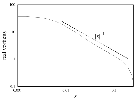
Figure 10: Same data as in the right half of Fig. 9 (c) in log-log coordinates. To obtain a better scaling, we subtract a constant (here $2.0$) from the real part of the vorticity.

It is also of interest to show the variation of the vorticity in the $(y_{1},\,y_{2})$-plane, that is $\omega_{\star}(y_{1},y_{2})\equiv\omega(\pi+iy_{1},\pi+iy_{2})$. Symmetry implies that this is a real quantity which, by (7), can be written as

$$\!\!\!\!\!\!\omega_{\star}(y_{1},y_{2}) = \sum_{k_{1}=-\infty}^{0}\sum_{k_{2}=-\infty}^{0}(-1)^{k_{1}}k^{2}\,\hat{F}_{k_{1},\,k_{2}}\,e^{\,-(k_{1}y_{1}+k_{2}y_{2})\,},$$ (18)

$$k^{2} = k_{1}^{2}+k_{2}^{2}.$$

The latter can be viewed as a double power series in the variables $w_{1}\equiv e^{y_{1}}$ and $w_{2}\equiv e^{y_{2}}$. The alternating sign property of the $\hat{F}_{k_{1},\,k_{2}}$ mentioned at the end of Section 3 implies that all the coefficients $(-1)^{k_{1}}k^{2}\,\hat{F}_{k_{1},\,k_{2}}$ are nonnegative for $k_{1}<-1$. It is well known that if a power series in one variable with nonnegative coefficients defines an analytic function with singularities, then the nearest singularity to the origin is on the real positive axis (Vivanti’s theorem, see, e.g., Dienes, 1931). Here we expect that there will be a whole singular curve in the $(y_{1},\,y_{2})$-plane. The Fourier series can be used to calculate $\omega_{\star}(y_{1},y_{2})$, at least within the disk $y_{1}^{2}+y_{2}^{2}<\delta^{2}$. Fig. 11 shows contours

Figure 11: Contours of the vorticity $\omega_{\star}(y_{1},\,y_{2})$ for $x_{1}=\pi$ and $x_{2}=\pi$. The dotted circle has radius $\delta=0.0065$, whose smallness makes the contours nearly straight. Contour values from lower left to upper right are $30,40,\ldots,90,100,200$ (the thick solid line is for $100$).

of $\omega_{\star}$ in and around this disk. The contours are almost straight lines perpendicular to the most singular direction, because $\delta$ is very small. The variation of $\omega_{\star}$ along the the most singular direction as a function of the distance $y$ to the origin is shown in Fig. 12. When plotted as a function of the distance $\delta-y$ to the nearest singularity $(y_{1\star},\,y_{2\star})=\delta(\cos\theta_{\star},\,\sin\theta_{\star})$, it follows roughly a power law with an exponent close to $-3/4$ over almost two decades. We observe that the vorticity reaches values around 200. Peak values between 100 and 200 and a scaling exponent close to $-3/4$ are also obtained for the behavior of $\omega_{\star}$ near other points of the singular manifold (to be defined precisely in the next section). We observe that there may be an inconsistency between the exponent observed in the real direction which is roughly $-1$ (Fig. 10) and the exponent $-3/4$ observed in the imaginary direction (Fig. 12) since the vorticity, being analytic, should have the same scaling. The singularities being contained in the imaginary plane above $x_{1}=\pi,\,x_{2}=\pi$, at least a few meshes away from the real domain, the scaling in the imaginary direction is expected to be more reliable.

Actually, there is strong evidence for the vorticity being infinite at $(y_{1\star},\,y_{2\star})$ coming from the behavior of the shell-summed amplitudes. Indeed, we know (i) that all the terms in the double sum (18) are nonnegative and (ii) that the shell-summed stream function amplitude decreases nearly as $k^{-2}$ over two decades or more (Fig. 7). It follows that the shell-sums for the vorticity at $(y_{1\star},\,y_{2\star})$ are almost $k$-independent and thus, when we sum over $k$, we get an infinite value.

Figure 12: Vorticity $\omega_{\star}$ along the most singular direction as a function of the distance $\delta-y$ to the singularity nearest to the real domain.

5 The singular manifold

In one dimension it is well known that the high-wavenumber asymptotics of the Fourier transform of an analytic periodic function is governed by the singularities nearest to the real domain (see, e.g., Carrier, Krook and Pearson, 1966; Frisch and Morf, 1981). This has a non-trivial extension to more than one dimension when the function has singularities on a complex manifold ${\mathcal{S}}$ determined by an equation $S({\bm{z}})=0$; let us sketch this in the two-dimensional case. Consider a periodic analytic function $F({\bm{z}})$ given by the Fourier series (7). The Fourier coefficients are given by the double integral over the real periodicity domain

$$\hat{F}_{k_{1},k_{2}}=\frac{1}{(2\pi)^{2}}\int\int dx_{1}dx_{2}\,e^{-i(k_{1}x_{1}+k_{2}x_{2})}F({\bm{x}}).$$ (19)

Let us set $k_{1}=k\cos\theta$ and $k_{2}=k\sin\theta$. We are interested in the behavior of $\hat{F}_{k_{1},k_{2}}$ when $k\to\infty$ for a given direction defined by the angle $\theta$. For this we change coordinates from $(x_{1},\,x_{2})$ to $(x_{\|},\,x_{\perp})$ chosen, respectively, parallel and perpendicular to ${\bm{k}}$. Note that the exponential in (19) involves only $x_{\|}$. Hence (19) can be rewritten as a one-dimensional Fourier transform

$$\hat{F} = \frac{1}{2\pi}\int dx_{\|}\,e^{-ikx_{\|}}g_{\theta}(x_{\|})$$ (20)

$$g_{\theta}(x_{\|}) \equiv \frac{1}{2\pi}\int dx_{\perp}\,F(x_{\|}\hat{\bm{k}}+x_{\perp}\hat{\bm{k}}_{\perp}),$$ (21)

where $\hat{\bm{k}}\equiv{\bm{k}}/k$ and $\hat{\bm{k}}_{\perp}$ is $\hat{\bm{k}}$ rotated by $+\pi/2$. It follows from (20) that, for $k\to\infty$, $\hat{F}\sim e^{-ikz^{\star}_{\|}}$ where $z^{\star}_{\|}$ is the singularity of $g_{\theta}(z_{\|})$ in the complex $z_{\|}$ plane nearest to the real domain and with negative imaginary part. Hence $|\hat{F}|\sim e^{-k\delta(\theta)}$ where $\delta(\theta)=-{\rm Im}\,z^{\star}_{\|}$.

How do we obtain the singularities of $g_{\theta}(z_{\|})$, given by the integral (21)? For some (complex) $z_{\|}$ there may be singularities of $F(z_{\|}\hat{\bm{k}}+z_{\perp}\hat{\bm{k}}_{\perp})$ for real $z_{\perp}$. They can however be avoided by shifting the contour of integration away from the real $z_{\perp}$ axis. If we change $z_{\|}$, this will work as long as the contour does not get pinched between two (or more) coalescing singularities (the pinching, generically, does not take place on the real $z_{\perp}$ axis). Assuming that the singular manifold ${\mathcal{S}}$ can be represented by $S_{\theta}(z_{\|},z_{\perp})=0$ in the $z_{\|}$ and $z_{\perp}$ variables, a necessary condition for this pinching is a double root in $z_{\perp}$, i.e. $S_{\theta}=0$ and $\partial S_{\theta}/\partial z_{\perp}=0$. This system of two equations has discrete solutions $(z^{\star}_{\|},\,z^{\star}_{\perp})$, one of which will control the asymptotics. In an earlier version of this paper (available at http://arxiv.org/pdf/nlin.CD/0310044v1) we stated that the pinching argument may already be known. Recently W. Pauls pointed out to us that it has already been used in a special case by Henri Poincaré (see Sections 94–96 of Poincaré, 1899) and has later been generalized by Tsikh (1993).

All this simplifies considerably for the function $F$, the solution of the similarity equation. Indeed, all the relevant singularities have real part at the point $(\pi,\,\pi)$ and we can restrict everything to the pure imaginary plane $(y_{1},\,y_{2})$ passing through this point. Let the restriction of the singular manifold to this plane have the parametric representation $y_{1}(\theta),\,y_{2}(\theta)$, where $y_{1}$ and $y_{2}$ are differentiable functions of the parameter $\theta$, chosen in such a way that the angle between the $y_{1}$ axis and the tangent at the singular manifold is $\theta+\pi/2$. We obviously have

$$\frac{dy_{2}}{dy_{1}}=-\frac{1}{\tan\theta}.$$ (22)

This representation is convenient because the aformentioned condition of having a double root is easily shown to express the tangency to the singular manifold of the straight line perpendicular to the direction $\theta-\pi$ at a distance $\delta(\theta)$ from the origin, as illustrated in Fig. 13.

Figure 13: Geometrical determination of the logarithmic decrement $\delta(\theta)$ associated to the direction $\theta$ in terms of the singular manifold in the $(y_{1},\,y_{2})$-plane.

Figure 14: The singular manifold in the $(y_{1},\,y_{2})$-plane constructed as an envelope of numerically determined analyticity disks for 305 different choices of parareal planes. Inset: enlargement near the origin.

The equation for the tangent reads

$$\delta(\theta)=y_{1}\cos(\theta-\pi)+y_{2}\sin(\theta-\pi).$$ (23)

The system (22)-(23) is easily inverted (provided the singular manifold restricted to the $(y_{1},\,y_{2})$-plane is convex) to give

$$y_{1}(\theta) = -\delta(\theta)\cos\theta+\delta^{\prime}(\theta)\sin\theta$$ (24)

$$y_{2}(\theta) = -\delta(\theta)\sin\theta-\delta^{\prime}(\theta)\cos\theta,$$ (25)

where $\delta^{\prime}(\theta)\equiv d\delta(\theta)/d\theta$.

These equations allow in principle the construction of the singular manifold from the knowledge of the angular dependence of the logarithmic decrement $\delta(\theta)$, as given in Fig. 6.

In practice, because $\delta(\theta)$ changes very quickly near its minimum, this is not a very well conditioned procedure. An alternative construction by envelope of analyticity disks is now proposed. We observe that, when we replace the real plane by a parareal plane shifted by an imaginary vector $(h_{1},\,h_{2})$, the location on the singular manifold nearest to this parareal plane is generically different from the one nearest to the original real plane. For a general 2D problem without special symmetry, the singular manifold is a one-dimensional complex manifold, and thus may be parametrized with two real variables, e.g. $h_{1}$ and $h_{2}$. For the special case considered here, we can work in the $(y_{1},\,y_{2})$ plane and draw around each point $(h_{1},\,h_{2})$ an analyticity disk of radius $\delta(h_{1},h_{2})$. The latter is determined as the logarithmic decrement of the shell-summed average of $\exp(k_{1}h_{1}+k_{2}h_{2})\hat{F}_{k_{1},k_{2}}$, where the exponential factor is the consequence in Fourier space of the imaginary translation $(ih_{1},\,ih_{2})$. It is easily shown that

$$\delta(h_{1},h_{2})=\min_{\theta}\,\left(\delta(\theta)-h_{1}\cos\theta-h_{2}\sin\theta\right),$$ (26)

where $\delta(\theta)$ is the logarithmic decrement in the direction $\theta$, defined in Section 4. Since $\delta(\theta)$ is rather poorly determined, it is better to measure $\delta(h_{1},h_{2})$ directly. We perform this calculation for 305 choices of the pair $(h_{1},\,h_{2})$, taken on a regular grid. The shell-summed averages are fitted to an exponential with an algebraic prefactor. Only points displaying decreasing exponentials, i.e., located below the singular manifold are kept. The result is shown in Fig. 14, where the singular manifold emerges as the envelope of all the analyticity disks. Let us finally observe that the method of analyticity disks can be generalized to problems without any special symmetry; this will be discussed elsewhere.

6 Concluding remarks

Let us now summarize what we have learned about singularities for the similarity equation (5) governing the short-time asymptotics. First, we remind the reader that for one-dimensional problems, complex-space singularities can be at isolated points but need not: for nonintegrable ODE’s they often form fractal natural boundaries (Chang, Tabor and Weiss, 1982). In two dimensions or higher, isolated singularities are ruled out: the singular set is a complex manifold (or worse). In the present case, the evidence is that the singularities are on a smooth and probably analytic one-dimensional complex manifold. This was already conjectured in FMB on the basis of numerical results for the full time-dependent Euler equation. Now, we have an explicit construction of the singular manifold by the method of envelope of analyticity disks (Section 5), which gives strong numerical evidence for smoothness.

The very clean scaling we have observed for the Fourier transform of the solution near the singularity (Fig. 7) implies that the vorticity is infinite on the singular manifold Since in 2D the vorticity is conserved along Lagrangian fluid trajectories (both in the real and the complex domain), this result strongly suggests that the singular manifold is mapped to complex infinity by the inverse Lagrangian map.

We have studied here a special flow, whose two-mode initial condition given by (2) has a center of symmetry at $(\pi,\,\pi)$. Such symmetries are hard to avoid when using a minimal number of Fourier modes. At short times, the symmetry constrains the complex-space singularity nearest to the real domain to have the real part of its location at $(x_{1},\,x_{2})=(\pi,\,\pi)$. In FMB we have shown that this ceases to be the case at later times. We do of course hope that there is something universal in the nature of the singularities, be it only their very existence. We must however stress that in the present case we have a singular manifold with a continuous piece and not just isolated points when $(x_{1},\,x_{2})=(\pi,\,\pi)$. This is definitely non-generic, since a manifold with complex dimension 1 may be viewed as a two-dimensional real manifold in four-dimensional real space. When higher-order harmonics are added to the initial condition (2), the situation becomes more complicated and the short-time asymptotic equation will in general depend on the ratio $y_{2}/y_{1}$, that is on the direction in which the imaginary coordinates become large.

Let us finally point out that one particularly challenging problem is to actually prove that there are singularities in the complex domain: at the moment we are not aware of a single instance of a solution to the incompressible Euler equation with smooth initial data for which the existence of a singularity (real or complex) is demonstrated. In the present case, the proof may be facilitated by the observation made in Section 4 that, in the $(y_{1},\,y_{2})$-plane the vorticity is real and can be represented as a double power series with (apparently) nonnegative coefficients. A lower bound on these coefficient – which are obtained from the solutions of the recurrence relations (12) – could lead to such a proof.

Acknowledgments
We are grateful to Walter Pauls, Tetsuo Ueda and Vladislav Zheligovsky for useful remarks. Computational resources were provided by the Yukawa Institute (Kyoto). This research was supported by the European Union under contract HPRN-CT-2000-00162 and by the Indo-French Centre for the Promotion of Advanced Research (IFCPAR 2404-2). TM was supported by the Grant-in-Aid for Young Scientists [(B), 15740237, 2003] and the Grant-in-Aid for the 21st Century COE “Center for Diversity and Universality in Physics” from the Japanese Ministry of Education and received also partial support from the French Ministry of Education. JB acknowledges support from the National Science Foundation under Agreement No. DMS-9729992.

References

- Bailey (1995) Bailey, D.H., 1995. A fortran-90 based multiprecision system, RNR Technical Report RNR-94-013. See also http://crd.lbl.gov/dhbailey/
- Bardos, Benachour and Zerner (1976) Bardos, C., Benachour, S., Zerner, M., 1976. Analyticité des solutions periodiques de l’équation d’Euler en deux dimensions, C. R. Acad. Sc. Paris 282 A, 995–998.
- Bajer and Moffat (2003) Bajer, K., Moffatt, H.K. (ed), 2003. Tubes, Sheets and Singularities in Fluid Dynamics: Proceedings of the NATO ARW, 2–7 September 2001, Zakopane, Poland, Kluwer Academic Publishers, Dordrecht.
- Brachet et al. (1983) Brachet, M.-E., Meiron, D.I., Orszag, S.A., Nickel, B.G., Morf, R.H., Frisch, U., 1983. Small-scale structure of the Taylor-Green vortex, J. Fluid Mech. 130 411–452.
- Caflisch, Hou and Lowengrub (1999) Caflisch, R.E., Hou, T.Y., Lowengrub, J., 1999. Almost optimal convergence of the point vortex method for vortex sheets using numerical filtering, Math. Comput. 68, 1465–1496.
- Carrier, Krook and Pearson (1966) Carrier, G.F., Krook, M., Pearson, C.E., 1966. Functions of a complex variable: theory and technique, McGraw-Hill, New York.
- Chang, Tabor and Weiss (1982) Chang, Y.F., Tabor, M., Weiss, J., 1982. Analytic structure of the Hénon–Heiles hamiltonian in integrable and nonintegrable regimes, J. Math. Phys. 23, 531–538.
- Cramér (1938) Cramér, H., 1938. Sur un nouveau théorème-limite de la théorie des probabilités, Actualités Scientifiques et Industrielles, 736, 5–23
- Dienes (1931) Dienes, P., 1931. The Taylor Series, an Introduction to the Theory of Functions of a Complex Variable, Oxford University Press.
- Frisch (1984) Frisch, U., 1984. The analytic structure of turbulent flows, in Proceed. Chaos and statistical methods, Sept. 1983, Kyoto, Y. Kuramoto, ed. pp. 211–220, Springer.
- Frisch, Matsumoto and Bec (2003) Frisch, U., Matsumoto, T., Bec, J., 2003. Singularities of Euler flow? Not out of the blue! J. Stat. Phys. 113, 761–781.
- Frisch and Morf (1981) Frisch, U., Morf, R., 1981. Intermittency in nonlinear dynamics and singularities at complex times, Phys. Rev. A 23, 2673–2705.
- Kida (1985) Kida, S., 1985. Three-dimensional periodic flows with high-symmetry, J. Phys. Soc. Japan 54, 2132–2136.
- Krasny (1986) Krasny, R., 1986. A study of singularity formation in a vortex sheet by the point-vortex approximation, J. Fluid Mech. 167, 65–93.
- Majda and Bertozzi (2001) Majda, A.J., Bertozzi, A.L., 2001. Vorticity and Incompressible Flow (Section 9.4), Cambridge Texts in Applied Mathematics, Cambridge University Press, Cambridge.
- Pauls and Matsumoto (2005) Pauls, W., Matsumoto, T., 2005. Lagrangian singularities of steady two-dimensional flow, Geophys. Astrophys. Fluid Dynam. 99, 61–75.
- Pelz (1997) Pelz, R.B., 1997. Locally self-similar, finite-time collapse in a high-symmetry vortex filament model, Phys. Rev. E 55, 1617–1626.
- Pelz (2001) Pelz, R.B., 2001. Symmetry and the hydrodynamic blow-up problem, J. Fluid Mech. 444, 299–320.
- Pelz and Gulak (1997) Pelz, R.B., Gulak, Y., 1997. Evidence for a real-time singularity in hydrodynamics from time series analysis, Phys. Rev. Lett. 79, 4998–5001.
- Poincaré (1899) Poincaré, H., 1899. Les Méthodes Nouvelles de la Mécanique Céleste, Gauthier-Villars, Paris reprinted by Dover in 1957.
- Sulem, Sulem and Frisch (1983) Sulem, C., Sulem, P.-L., Frisch, H., 1983. Tracing complex singularities with spectral methods, J. Comput. Phys. 50, 138–161.
- Tsikh (1993) Tsikh, A., 1993. Conditions for absolute convergence of series of Taylor coefficients of meromorphic functions of two variables, Math. USSR Sbornik 74, 336–360.