Symmetries of Discrete Systems

Abstract

In this series of lectures, presented at the CIMPA Winter School on Discrete Integrable Systems in February 2003, we give a review of the application of Lie point symmetries, and their generalizations, to the study of difference equations. The overall theme could be called “continuous symmetries of discrete equations”.

1 Introduction

1.1 Symmetries of Differential Equations

Before studying the symmetries of difference equations, let us very briefly review the theory of the symmetries of differential equations. For all details, proofs and further information we refer to the many excellent books on the subject e.g. [48, 7, 49, 31, 22, 3, 53, 58].

Let us consider a completely general system of differential equations

$$E_{a}(x,u,u_{x},u_{xx},\dots u_{nx})=0,\quad x\in\mathbf{R}^{p},u\in\mathbf{R}^{q},a=1,\dots N,$$ (1)

where e.g. $u_{nx}$ denotes all (partial) derivatives of order $n$. The numbers $p,q,n$ and $N$ are all nonnegative integers.

We are interested in the symmetry group $G$ of the system (1), i.e. in the local Lie group of local point transformations taking solutions of eq. (1) into solutions. Point transformations in the space $X\times U$ of independent and dependent variables have the form

$$\tilde{x}=\Lambda_{\lambda}(x,u),\quad\tilde{u}=\Omega_{\lambda}(x,u),$$ (2)

where $\lambda$ denotes the group parameters. We have

$$\Lambda_{0}(x,u)=x,\quad\Omega_{0}(x,u)=u$$

and the inverse transformation $(\tilde{x},\tilde{u})\to(x,u)$ exists, at least locally.

The transformations (2) of local coordinates in $X\times U$ also determine the transformations of functions $u=f(x)$ and of derivatives of functions. A group $G$ of local point transformations of $X\times U$ will be a symmetry group of the system (1) if the fact that $u(x)$ is a solution implies that $\tilde{u}(\tilde{x})$ is also a solution.

The two fundamental questions to ask are:

1. How to find the maximal symmetry group $G$ for a given system of equations (1)?

2. Once the group $G$ is found, what do we do with it?

Let us first discuss the question of motivation. The symmetry group $G$ allows us to do the following.

1. Generate new solutions from known ones. Sometimes trivial solutions can be boosted into interesting ones.

2. Identify equations with isomorphic symmetry groups. Such equations may be transformable into each other. Sometimes nonlinear equations can be transformed into linear ones.

3. Perform symmetry reduction: reduce the number of variables in a PDE and obtain particular solutions, satisfying particular boundary conditions: group invariant solutions. For ODEs of order $n$, we can reduce the order of the equation. In this reduction, there is no loss of information. If we can reduce the order to zero, we obtain a general solution depending on $n$ constants, or a general integral (an algebraic equation depending on $n$ constants).

How does one find the symmetry group $G$? One looks for infinitesimal transformations, i.e. one looks for the Lie algebra $L$ that corresponds to $G$. Instead of looking for “global” transformations as in eq. (2) one looks for infinitesimal ones. A one-parameter group of infinitesimal point transformations will have the form

$$\tilde{x}_{i} = x_{i}+\lambda\xi_{i}(x,u)\quad|\lambda|<<1$$ (3)

$$\tilde{u}_{\alpha} = u_{\alpha}+\lambda\phi_{\alpha}(x,u)\quad 1\leq i\leq p,\quad 1\leq\alpha\leq q.$$

The functions $\xi_{i}$ and $\phi_{\alpha}$ must be found from the condition that $\tilde{u}(\tilde{x})$ is a solution whenever $u(x)$ is one. The derivatives $\tilde{u}_{\alpha,\tilde{x}_{i}}$ must be calculated using eq. (3) and will involve derivatives of $\xi_{i}$ and $\phi_{\alpha}$. A $K$-th derivative of $\tilde{u}_{\alpha}$ with respect to the variable $\tilde{x}_{i}$ will involve derivatives of $\xi_{i}$ and $\phi_{\alpha}$ up to order $K$. We then substitute the transformed quantities into eq. (1) and request that the equation be satisfied for $\tilde{u}(\tilde{x})$, whenever it is satisfied for $u(x)$. Thus, terms of order $\lambda^{0}$ will drop out. Terms of order $\lambda$ will provide a system of determining equations for $\xi_{i}$ and $\phi_{\alpha}$. Terms of order $\lambda^{k}$, $k=2,3,\dots$ are to be ignored, since we are looking for infinitesimal symmetries.

The functions $\xi_{i}$ and $\phi_{\alpha}$ depend only on $x$ and $u$, not on first, or higher derivatives, $u_{\alpha,x_{i}}$, $u_{\alpha,x_{i}x_{k}}$, etc. This is actually the definition of “point” symmetries. The determining equations will explicitly involve derivatives of $u_{\alpha}$, up to the order $n$ (the order of the studied equation). The coefficients of all linearly independent expressions in the derivatives must vanish separately. This provides a system of determining equations for the functions $\xi_{i}(x,u)$ and $\phi_{\alpha}(x,u)$. This is a system of linear partial differential equations of order $n$. The determining equations are linear, even if the original system (1) is nonlinear. This “linearization” is due to the fact that all terms of order $\lambda^{j}$, $j\geq 2$, are ignored.

The system of determining equations is usually overdetermined, i.e. there are usually more determining equations than unknown functions $\xi_{i}$ and $\phi_{\alpha}$ ($p+q$ functions). The independent variables in the determining equations are $x\in\mathbf{R}^{p}$, $u\in\mathbf{R}^{q}$.

For an overdetermined system, three possibilities occur.

1. The only solution is the trivial one $\xi_{i}=0$, $\phi_{\alpha}=0$, $i=1,\dots p,\alpha=1,\dots,q$. In this case the symmetry algebra is $L=\{0\}$, the symmetry group is $G=I$ and the symmetry method is to no avail.

2. The general solution of the determining equations depends on a finite number $K$ of constants. In this case the studied system (1) has a finite-dimensional Lie point symmetry group and we have $\dim G=K$.

3. The general solution depends on a finite number of arbitrary functions of some of the variables $\{x_{i},u_{\alpha}\}$. In this case the symmetry group is infinite dimensional. This last case is of particular interest.

The search for the symmetry algebra $L$ of a system of differential equations is best formulated in terms of vector fields acting on the space $X\times U$ of independent and dependent variables. Indeed, consider the vector field

$$X=\sum^{p}_{i=1}\xi_{i}(x,u)\partial x_{i}+\sum^{q}_{\alpha=1}\phi_{\alpha}(x,u)\partial u_{\alpha},$$ (4)

where the coefficients $\xi_{i}$ and $\phi_{\alpha}$ are the same as in eq. (3). If these functions are known, the vector field (4) can be integrated to obtain the finite transformations (2). Indeed, all we have to do is integrate the equations

$$\frac{d\tilde{x}_{i}}{d\lambda}=\xi_{i}(\tilde{x},\tilde{u}),\quad\frac{d\tilde{u}_{\alpha}}{d\lambda}=\phi_{\alpha}(\tilde{x},\tilde{u}),$$ (5)

subject to the initial conditions

$$\tilde{x}_{i}\mid_{\lambda=0}=x_{i}\quad\tilde{u}_{\alpha}\mid_{\lambda=0}=u_{\alpha}.$$ (6)

This provides us with a one-parameter group of local Lie point transformations of the form (2) with $\lambda$ the group parameter.

The vector field (4) tells us how the variables $x$ and $u$ transform. We also need to know how derivatives like $u_{x}$, $u_{xx}$, $\dots$ transform. This is given by the prolongation of the vector field $X$.

We have

$$\mathop{\mathrm{pr}}\nolimits X=X+\sum_{\alpha}\biggl{\{}\sum_{i}\phi^{x_{i}}_{\alpha}\partial u_{x_{i}}+\sum_{i,k}\phi^{x_{i}x_{k}}_{\alpha}\partial u_{x_{i}x_{k}}$$

$$+\sum^{x_{i}x_{k}x_{l}}_{i,k,l}\phi_{\alpha}\partial u_{x_{i}x_{k}x_{l}}+\dots\biggr{\}},$$

where the coefficients in the prolongation can be calculated recursively, using the total derivative operator

$$D_{x_{i}}=\partial_{x_{i}}+u_{\alpha,x_{i}}\partial_{u_{\alpha}}+u_{\alpha,x_{a}x_{i}}\partial_{u_{\alpha},x_{a}}+u_{\alpha,x_{a}x_{b}x_{i}}\partial_{u_{\alpha},x_{a}x_{b}}+\dots$$ (8)

(a summation over repeated indices is to be understood).

The recursive formulas are

$$\phi^{x_{i}}_{\alpha} = D_{x_{i}}\phi_{\alpha}-(D_{x_{i}}\xi_{a})u_{\alpha,x_{a}}$$

$$\phi^{x_{i}x_{k}}_{\alpha} = D_{x_{k}}\phi^{x_{i}}_{\alpha}-(D_{x_{k}}\xi_{a})u_{\alpha,x_{i}x_{a}}$$ (9)

$$\phi^{x_{i}x_{k}x_{l}}_{\alpha} = D_{x_{l}}\phi^{x_{i}x_{k}}_{\alpha}-(D_{x_{l}}\xi_{a})u_{\alpha,x_{i}x_{k}x_{a}}$$

etc.

The $n$-th prolongation of $\widehat{X}$ acts on functions of $x$, $u$ and all derivatives of $u$ up to order $n$. It also tells us how derivatives transform. Thus, to obtain the transformed quantities $\tilde{u}_{\tilde{x}_{i}}$ we must integrate eq. (5) with conditions (6), together with

$$\frac{d\tilde{u}_{\tilde{x}_{i}}}{d\lambda}=\phi^{x_{i}}(\tilde{x},\tilde{u},\tilde{u}_{\tilde{x}}),\quad\tilde{u}_{\tilde{x}}\mid_{\lambda=0}=u_{x}.$$ (10)

We see that the coefficients of the prolonged vector field are expressed in terms of derivatives of $\xi_{i}$ and $\phi_{\alpha}$, the coefficients of the original vector field. They carry no new information: the transformation of derivatives is completely determined, once the transformations of functions are known.

The invariance condition for the system (1) is expressed in terms of the operator (1.1) as

$$\mathop{\mathrm{pr}}\nolimits^{(n)}XE_{a}\mid_{E_{1}=\dots=E_{N}=0}=0,\quad a=1,\dots N,$$ (11)

where $\mathop{\mathrm{pr}}\nolimits^{(n)}X$ is the prolongation (1.1) calculated up to order $n$ where $n$ is the order of the system (1).

In practice the symmetry algorithm consists of several steps, most of which can be carried out on a computer. For early computer programs calculating symmetry algebras, see Ref. [56, 9]. For a more recent review, see [25].

The individual steps are:

1. Calculate all the coefficients in the $n$-th prolongation of $\widehat{X}$. This depends only on the order of the system (1), i.e. $n$, and on the number of independent and dependent variables, i.e. $p$ and $q$.

2. Consider the system (1) as a system of algebraic equations for $x$, $u$, $u_{x}$, $u_{xx}$, etc. Choose $N$ variables $v_{1}$, $v_{2}$, $\dots v_{N}$ and solve the system (1) for these variables. The $v_{i}$ must satisfy the following conditions.

   1. Each $v_{i}$ is a derivative of one $u_{\alpha}$ of at least order 1.

   2. The variables $v_{i}$ are all independent, none of them is a derivative of any other one.

   3. No derivatives of any of the $v_{i}$ figure in the system (1).

3. Apply $\mathop{\mathrm{pr}}\nolimits^{(n)}X$ to all the equations in (1) and eliminate all expressions $v_{i}$ from the result. This provides us with the system (11).

4. Determine all linearly independent expressions in the derivatives remaining in (11), once the quantities $v_{i}$ are eliminated. Set the coefficients of these expressions equal to zero. This provides us with the determining equations, a system of linear partial differential equations of order $n$ for $\phi_{\alpha}(x,u)$ and $\xi_{i}(x,u)$.

5. Solve the determining equations to obtain the symmetry algebra.

6. Integrate the obtained vector fields to obtain the one-parameter subgroups of the symmetry group. Compose them appropriately to obtain the connected component $G_{o}$ of the symmetry group $G$.

7. Extend the connected component $G_{o}$ to the full group $G$ by adding all discrete transformations leaving the system (1) invariant. These discrete transformations will form a finite, or discrete group $G_{D}$. We have

   $$G=G_{D}\mathbin{\hbox to0.0pt{\raisebox{0.1pt}{$\times$}\hss}\mskip-4.0mu\supset}G_{o}$$ (12)

   i.e. $G_{o}$ is an invariant subgroup of $G$.

Let us consider the case when at Step 5 we obtain a finite dimensional Lie algebra $L$, i.e. a vector field $X$ depending on $K$ parameters, $K\in\mathbf{Z}^{>}$, $K<\infty$. We can then choose a basis

$$\{X_{1},X_{2},\dots,X_{K}\}$$ (13)

of the Lie algebra $L$. The basis that is naturally obtained in this manner depends on our integration procedure, though the algebra $L$ itself does not. It is useful to transform the basis (13) to a canonical form in which all basis independent properties of $L$ are manifest. Thus, if $L$ can be decomposed into a direct sum of indecomposable components,

$$L=L_{1}\oplus L_{2}\oplus\dots\oplus L_{M},$$ (14)

then a basis should be chosen that respects this decomposition. The components $L_{i}$ that are simple should be identified according to the Cartan classification (over $\mathbf{C}$) or the Gantmakher classification (over $\mathbf{R}$) [47, 24]. The components that are solvable should be so organized that their nilradical [52, 32] is manifest. For those components that are neither simple, nor solvable, the basis should be chosen so as to respect the Levi decomposition [52, 32].

So far we have considered only point transformations, as in eq. (2), in which the new variables $\tilde{x}$ and $\tilde{u}$ depend only on the old ones, $x$ and $u$. More general transformations are “contact transformations”, where $\tilde{x}$ and $\tilde{u}$ also depend on first derivatives of $u$. A still more general class of transformations are generalized transformations, also called “Lie-Bäcklund” transformations [48, 4]. For these we have

$$\tilde{x} = \Lambda_{\lambda}(x,u,u_{x},u_{xx},\dots)$$ (15)

$$\tilde{u} = \Omega_{\lambda}(x,u,u_{x},u_{xx},\dots)$$

involving derivatives up to an arbitrary order. The coefficients $\xi_{i}$ and $\phi_{\alpha}$ of the vector fields (4) will then also depend on derivatives of $u_{\alpha}$.

When studying generalized symmetries, and sometimes also point symmetries, it is convenient to use a different formalism, namely that of evolutionary vector fields.

Let us first consider the case of Lie point symmetries, i.e. vector fields of the form (4) and their prolongations (1.1). To each vector field (4) we can associate its evolutionary counterpart $X_{e}$, defined as

$$X_{e} = Q_{\alpha}(x,u,u_{x})\partial u_{\alpha},$$ (16)

$$Q_{\alpha} = \phi_{\alpha}-\xi_{i}\frac{\partial u_{\alpha}}{\partial x_{i}}.$$ (17)

The prolongation of the evolutionary vector field (16) is defined as

$$\mathop{\mathrm{pr}}\nolimits X_{e} = Q_{\alpha}\partial u_{a}+Q^{x_{i}}_{\alpha}\partial u_{\alpha,x_{i}}+Q^{x_{i}x_{k}}_{\alpha}\partial u_{\alpha,x_{i}x_{k}}+\dots$$ (18)

$$Q^{x_{i}}_{\alpha} = D_{x_{i}}Q_{\alpha},\quad Q^{x_{i}x_{k}}_{\alpha}=D_{x_{i}}D_{x_{k}}Q_{\alpha},\dots.$$

The functions $Q_{\alpha}$ are called the characteristics of the vector field. Notice that $X_{e}$ and $\mathop{\mathrm{pr}}\nolimits X_{e}$ do not act on the independent variables $x_{i}$.

For Lie point symmetries evolutionary and ordinary vector fields are entirely equivalent and it is easy to pass from one to the other. Indeed, eq. (17) gives the connection between the two.

The symmetry algorithm for calculating the symmetry algebra $L$ in terms of evolutionary vector fields is also equivalent. Eq. (11) is simply replaced by

$$\mathop{\mathrm{pr}}\nolimits^{(n)}X_{e}E_{a}\mid_{E_{1}=\dots=E_{N}=0},=0,\quad a=1,\dots N.$$ (19)

The reason that eq. (11) and (19) are equivalent is the following. It is easy to check that we have

$$\mathop{\mathrm{pr}}\nolimits^{(n)}X_{e}=\mathop{\mathrm{pr}}\nolimits^{(n)}X-\xi_{i}D_{i}.$$ (20)

The total derivative $D_{i}$ is itself a generalized symmetry of eq. (1), i.e. we have

$$D_{i}E_{a}\mid_{E_{1}=E_{2}=\dots=E_{n}=0},=0\quad i=1,\dots p,\quad a=1,\dots N.$$ (21)

Eq. (20) and (21) prove that the systems (11) and (19) are equivalent. Eq. (21) itself follows from the fact that $DE_{a}=0$ is a differential consequence of eq. (1), hence every solution of eq. (1) is also a solution of eq. (21).

To find generalized symmetries of order $k$ we use eq. (16) but allow the characteristics $Q_{\alpha}$ to depend on all derivatives of $u_{\alpha}$ up to order $k$. The prolongation is calculated using eq. (18). The symmetry algorithm is again eq. (19).

A very useful property of evolutionary symmetries is that they provide compatible flows. This means that the system of equations

$$\frac{\partial u_{\alpha}}{\partial\lambda}=Q_{\alpha}$$ (22)

is compatible with the system (1). In particular, group invariant solutions, i.e. solutions invariant under a subgroup of $G$ are obtained as fixed points

$$Q_{\alpha}=0.$$ (23)

If $Q_{\alpha}$ is the characteristic of a point transformation then (23) is a system of quasilinear first order partial differential equations. They can be solved, the solution substituted into (1) and this provides the invariant solutions explicitly.

1.2 Comments on Symmetries of Difference Equations

The study of symmetries of difference equations is much more recent than that of differential equations. Early work in this direction is due to Maeda [44, 45] who mainly studied transformations acting on the dependent variables only. A more recent series of papers was devoted to Lie point symmetries of differential-difference equations on fixed regular lattices [40, 41, 42, 23, 34, 33, 46, 50, 51, 8]. A different approach was developed mainly for linear or linearizable difference equations and involved transformations acting on more than one point of the lattice [20, 21, 39, 28, 36]. The symmetries considered in this approach are really generalized ones, however they reduce to point ones in the continuous limit.

A more general class of generalized symmetries has also been investigated for difference equations, and differential-difference equations on fixed regular lattices [26, 27, 29, 35].

A different approach to symmetries of discrete equations was originally suggested by V. Dorodnitsyn and collaborators [11, 13, 12, 5, 15, 14, 19, 16, 18, 17]. The main aim of this series of papers is to discretize differential equations while preserving their Lie point symmetries.

Symmetries of ordinary and partial difference schemes on lattices that are a priori given, but are allowed to transform under point transformations, were studied in Ref. [37, 38, 43].

2 Ordinary Difference Schemes and Their Point Symmetries

2.1 Ordinary Difference Schemes

An ordinary differential equation (ODE) of order $n$ is a relation involving one independent variable $x$, one dependent variable $u=u(x)$ and $n$ derivatives $\stackrel{{\scriptstyle\prime}}{{u}}$, $\stackrel{{\scriptstyle\prime\prime}}{{u}}$, $\dots u^{(n)}$

$$E(x,u,\stackrel{{\scriptstyle\prime}}{{u}},\stackrel{{\scriptstyle\prime\prime}}{{u}},\dots,u^{(n)})=0\quad\frac{\partial E}{\partial u^{(n)}}\neq 0.$$ (24)

An ordinary difference scheme (O$\Delta$S) involves two objects, a difference equation and a lattice. We shall specify an O$\Delta$S by a system of two equations, both involving two continuous variables $x$ and $u(x)$, evaluated at a discrete set of points $\{x_{n}\}$.

Thus, a difference scheme of order $K$ will have the form

$$\begin{array}[]{c}E_{a}(\{x_{k}\}^{n+N}_{k=n+M},\{u_{k}\}^{n+N}_{k=n+M})=0,a=1,2\\[3.0pt] K=N-M+1,\quad n,M,N\in\mathbf{Z},\quad u_{k}\equiv u(x_{k}).\end{array}$$ (25)

At this stage we are not imposing any boundary conditions, so the reference point $x_{n}$ can be arbitrarily shifted to the left, or to the right. The order $K$ of the system is the number of points involved in the scheme (25) and it is assumed to be finite. We also assume that if the values of $x_{k}$ and $u_{k}$ are specified in $(N-M)$ neighbouring point, we can calculate their values in the point to the right, or to the left of the given set, using equations (25).

A continuous limit for the spacings between all neighbouring points going to zero, if it exists, will take one of the equations (25) into a differential equation of order $K^{\prime}\leq K$, another into an identity (like $0=0$).

When taking the continuous limit it is convenient to introduce different quantities, namely differences between neighbouring points and discrete derivatives like

$$h_{+}(x_{n}) = x_{n+1}-x_{n},\quad h_{-}(x_{n})=x_{n}-x_{n-1},$$

$$u_{,x} = \frac{u_{n+1}-u_{n}}{x_{n+1}-x_{n}},\quad u_{,\underline{x}}=\frac{u_{n}-u_{n-1}}{x_{n}-x_{n-1}},$$ (26)

$$u_{,x\underline{x}} = 2\frac{u_{,x}-u_{,\underline{x}}}{x_{n+1}-x_{n-1}},\dots$$

In the continuous limit, we have

$$h_{+}\to 0,\quad h_{-}\to 0,\quad u_{,{x}}\to\stackrel{{\scriptstyle\prime}}{{u}},\quad u_{,{\underline{x}}}\to\stackrel{{\scriptstyle\prime}}{{u}},\quad u_{,x\underline{x}}\to\stackrel{{\scriptstyle\prime\prime}}{{u}}.$$

As a clarifying example of the meaning of the difference scheme (25), let us consider a three point scheme that will approximate a second order linear difference equation:

$$E_{1} = \frac{u_{n+1}-2u_{n}+u_{n-1}}{(x_{n+1}-x_{n})^{2}}-u_{n}=0,$$ (27)

$$E_{2} = x_{n+1}-2x_{n}+x_{n-1}=0.$$ (28)

The solution of eq. $E_{2}=0$, determines a uniform lattice

$$x_{n}=hn+x_{0}$$ (29)

The scale $h$ and the origin $x_{0}$ in eq. (29) are not fixed by eq. (28), instead they appear as integration constants, i.e. they are a priori arbitrary. Once they are chosen, eq. (27) reduces to a linear difference equation with constant coefficients, since we have $x_{n+1}-x_{n}=h$. Thus, a solution of eq. (27) will have the form

$$u_{n}=\lambda^{x_{n}}.$$ (30)

Substituting (30) into (27) we obtain the general solution of the difference scheme (27), (28) as

$$u(x_{n}) = c_{1}\lambda^{x_{n}}_{1}+c_{2}\lambda^{x_{n}}_{2},\quad x_{n}=hn+x_{0},$$ (31)

$$\lambda_{1,2} = \left(\frac{2+h^{2}\pm h\sqrt{4+h^{2}}}{2}\right)^{1/2}.$$

The solution (31) of the system (27), (28) depends on 4 arbitrary constants $c_{1}$, $c_{2}$, $h$ and $x_{0}$.

Now let us consider a general three point scheme of the form

$$E_{a}(x_{n-1},x_{n},x_{n+1},u_{n-1},u_{n},u_{n+1})=0,\quad a=1,2$$ (32)

satisfying

$$\det\left(\frac{\partial(E_{1},E_{2})}{\partial(x_{n+1},u_{n+1})}\right)\neq 0,\quad\det\left(\frac{\partial(E_{1},E_{2})}{\partial(x_{n-1},u_{n-1})}\right)\neq 0,$$ (33)

(possibly after an up or down shifting). The two conditions on the Jacobians (33) are sufficient to allow us to calculate $(x_{n+1},u_{n+1})$ if $(x_{n-1},u_{n-1},x_{n},u_{n})$ are given. Similarly, $(x_{n-1},u_{n-1})$ can be calculated if $(x_{n},u_{n},x_{n+1},u_{n+1})$ are given. The general solution of the scheme (32) will hence depend on 4 arbitrary constants and will have the form

$$u_{n} = f(x_{n},c_{1},c_{2},c_{3},c_{4})$$ (34)

$$x_{n} = \phi(n,c_{1},c_{2},c_{3},c_{4}).$$ (35)

A more standard approach to difference equations would be to consider a fixed equally spaced lattice e.g. with spacing $h=1$. We can then identify the continuous variable $x$, sampled at discrete points $x_{n}$, with the discrete variable $n$:

$$x_{n}=n.$$ (36)

Instead of a difference scheme we then have a difference equation

$$E(\{u_{k}\}^{n+N}_{k=n+M})=0,$$ (37)

involving $K=N-M+1$ points. Its general solution has the form

$$u_{n}=f(n,c_{1},c_{2},\dots c_{N-M})$$ (38)

i.e. it depends on $N-M$ constants.

Below, when studying point symmetries of discrete equations we will see the advantage of considering difference systems like the system (25).

2.2 Point Symmetries of Ordinary Difference Schemes

In this section we shall follow rather closely the article [37]. We shall define the symmetry group of an ordinary difference scheme in the same manner as for ODEs. That is, a group of continuous local point transformations of the form (2) taking solutions of the O$\Delta$S (25) into solutions of the same scheme. The transformations considered are continuous, and we will adopt an infinitesimal approach, as in eq. (3). We drop the labels $i$ and $\alpha$, since we are considering the case of one independent and one dependent variable only.

As in the case of differential equations, our basic tool will be vector fields of the form (4). In the case of O$\Delta$S they will have the form

$$X=\xi(x,u)\partial_{x}+\phi(x,u)\partial_{u}$$ (39)

with

$$x\equiv x_{n},\quad u\equiv u_{n}=u(x_{n}).$$

Because we are considering point transformation, $\xi$ and $\phi$ in (39) depend on $x$ and $u$ at one point only.

The prolongation of the vector field $X$ is different than in the case of ODEs. Instead of prolonging to derivatives, we prolong to all points of the lattice figuring in the scheme (25). Thus we put

$$\mathop{\mathrm{pr}}\nolimits X=\sum^{n+N}_{k=n+M}\xi(x_{k},u_{k})\partial_{x_{k}}+\sum^{n+N}_{k=n+M}\phi(x_{k},u_{k})\partial_{u_{k}}.$$ (40)

In these terms the requirement that the transformed function $\tilde{u}(\tilde{x})$ should satisfy the same O$\Delta$S as the original $u(x)$ is expressed by the requirement

$$\mathop{\mathrm{pr}}\nolimits XE_{a}\mid_{E_{1}=E_{2}=0}=0,\quad a=1,2.$$ (41)

Since we must respect both the difference equation and the lattice, we have two conditions (41) from which to determine $\xi(x,u)$ and $\phi(x,u)$. Since each of these functions depends on a single point $(x,u)$ and the prolongation (40) introduces $N-M+1$ points in space $X\times U$, the equation (41) will imply a system of determining equations for $\xi$ and $\phi$. Moreover, in general this will be an overdetermined system of linear functional equations that we transform into an overdetermined system of linear differential equations [1, 2].

To illustrate the method and the role of the choice of the lattice, let us start from a simple example. The example will be that of difference equations that approximate the ODE

$$\stackrel{{\scriptstyle\prime\prime}}{{u}}=0$$ (42)

on several different lattices.

First of all, let us find the Lie point symmetry group of the ODE (42), i.e. the equation of a free particle on a line. Following the algorithm of Chapter 1, we put

$$\mathop{\mathrm{pr}}\nolimits^{(2)}X = \xi\partial_{x}+\phi\partial_{u}+\phi^{x}\partial_{\stackrel{{\scriptstyle\prime}}{{u}}}+\phi^{xx}\partial_{\stackrel{{\scriptstyle\prime\prime}}{{u}}}$$ (43)

$$\phi^{x} = D_{x}\phi-(D_{x}\xi)\stackrel{{\scriptstyle\prime}}{{u}}=\phi_{x}+(\phi_{u}-\xi_{x})\stackrel{{\scriptstyle\prime}}{{u}}-\xi_{u}\smash{\stackrel{{\scriptstyle\prime}}{{u}}}^{2}$$

$$\phi^{xx} = D_{x}\phi^{x}-(D_{x}\xi)\stackrel{{\scriptstyle\prime\prime}}{{u}}=\phi_{xx}+(2\phi_{xu}-\xi_{xx})\stackrel{{\scriptstyle\prime}}{{u}}$$

$$\quad+(\phi_{uu}-2\xi_{xu})\smash{\stackrel{{\scriptstyle\prime}}{{u}}}^{2}-\xi_{uu}\smash{\stackrel{{\scriptstyle\prime}}{{u}}}^{3}x+(\phi_{u}-2\xi_{x})\stackrel{{\scriptstyle\prime\prime}}{{u}}$$

$$\quad-3\xi_{u}v\stackrel{{\scriptstyle\prime}}{{u}}\stackrel{{\scriptstyle\prime\prime}}{{u}}.$$

The symmetry formula (11) in this case reduces to

$$\phi^{xx}\mid_{\stackrel{{\scriptstyle\prime\prime}}{{u}}=0}=0.$$ (44)

Setting the coefficients of $\smash{\stackrel{{\scriptstyle\prime}}{{u}}}^{3}$, $\smash{\stackrel{{\scriptstyle\prime}}{{u}}}^{2}$, $\stackrel{{\scriptstyle\prime}}{{u}}$ and $\smash{(\stackrel{{\scriptstyle\prime}}{{u}}}^{0})$ equal to zero, we obtain an 8 dimensional Lie algebra, isomorphic to $\mathop{\mathrm{sl}}(3,\mathbf{R})$ with basis

$$X_{1} = \partial_{x},\quad X_{2}=x\partial_{x},\quad X_{3}=u\partial_{x}$$ (45)

$$X_{4} = \partial_{u},\quad X_{5}=x\partial_{u},\quad X_{6}=u\partial_{u},$$

$$X_{7} = x(x\partial_{x}+u\partial_{u}),\quad X_{8}=u(x\partial_{x}+u\partial_{u}).$$

This result was of course already known to Sophus Lie. Moreover, any second order ODE that is linear, or linearizable by a point transformation has a symmetry algebra isomorphic to $\mathop{\mathrm{sl}}(3,\mathbf{R})$. The group $\mathop{\mathrm{SL}}(3,\mathbf{R})$ acts as the group of projective transformations of the Euclidean space $E_{2}$ (with coordinates $x,u)$).

Now let us consider some difference schemes that have eq. (42) as their continuous limit. We shall take the equation to be

$$\frac{u_{n+1}-2u_{n}+u_{n-1}}{(x_{n+1}-x_{n})^{2}}=0.$$ (46)

However before looking for the symmetry algebra, we multiply out the denominator and investigate the equivalent equation

$$E_{1}=u_{n+1}-2u_{n}+u_{n-1}=0.$$ (47)

To this equation we must add a second equation, specifying the lattice. We consider three different examples at first glance quite similar, but leading to different symmetry algebras.

Example 1.

Free particle (47) on a fixed uniform lattice. We take

$$E_{2}=x_{n}-hn-x_{0}=0,$$ (48)

where $h$ and $x_{0}$ are fixed constants (that are not transformed by the group (e.g. $h=1$, $x_{0}=0$).

Applying the prolonged vector field (40) to eq. (48) we obtain

$$\xi(x_{n},u_{n})=0$$ (49)

for all $x_{n}$ and $u_{n}$. Next, let us apply (40) to eq. (47) and replace $x_{n}$, using (48) and $u_{n+1}$, using (47). We obtain

$$\phi\big{(}h(n+1)+x_{0},2u_{n}-u_{n-1}\big{)}-2\phi(hn+x_{0},u_{n})$$ (50)

$$\hskip 54.92479pt+\phi\big{(}h(n-1)+x_{0},u_{n-1}\big{)}=0.$$

Differentiating eq. (50) twice, once with respect to $u_{n-1}$, once with respect to $u_{n}$, we obtain

$$\frac{\partial^{2}}{\partial u_{n+1}}\phi(x_{n+1},u_{n+1})=0$$ (51)

and hence

$$\phi(x_{n},u_{n})=A(x_{n})u_{n}+B(x_{n}).$$ (52)

We substitute eq. (52) back into (50) and equate coefficients of $u_{n}$, $u_{n-1}$ and 1. The result is

$$A(n+1)=A(n),\quad B(n+1)-2B(n)+B(n-1)=0.$$ (53)

Hence we have

$$A=A_{0},\quad B=B_{1}n+B_{0}=b_{1}x+b_{0}$$ (54)

where $A_{0}$, $B_{1}$, $B_{0}$, $b_{1}$ and $b_{0}$ are constants. We obtain the symmetry algebra of the O$\Delta$S (47), (48) and it is only three-dimensional, spanned by

$$X_{1}=\partial_{u},\quad X_{2}=x\partial_{u},\quad X_{3}=u\partial_{u}.$$ (55)

The corresponding one parameter transformation groups are obtained by integrating these vector fields (see eq. (5), (6))

$$G_{1} : \tilde{x}=x$$

$$\tilde{u}(\tilde{x})=u(x)+\lambda$$

$$G_{2} : \tilde{x}=x$$

$$\tilde{u}(\tilde{x})=u(x)+\lambda x$$

$$G_{3} : \tilde{x}=x$$

$$\tilde{u}(\tilde{x})=e^{\lambda}u(x)$$

$G_{1}$ and $G_{2}$ just tell us that we can add an arbitrary solution of the scheme to any given solution, $G_{3}$ corresponds to scale invariance of eq. (47).

Example 2.

Free particle (47) on a uniform two point lattice.

Instead of eq. (48) we define a lattice by putting

$$E_{2}=x_{n+1}-x_{n}=h,$$ (57)

where $h$ is a fixed (non-transforming) constant. Note that (57) tells us the distance between any two neighbouring points but does not fix an origin (as opposed to eq. (48)).

Applying the prolonged vector field (40) to eq. (57) and using (57), we obtain

$$\xi(x_{n}+h,u_{n+1})-\xi(x_{n},u_{n})=0.$$ (58)

Since $u_{n+1}$ and $u_{n}$ are independent, eq. (58) implies $\xi=\xi(x)$. Moreover $\xi(x_{n}+h)=\xi(x)$ so that we have

$$\xi=\xi_{0}=\mathop{\mathrm{const}}.$$ (59)

Further, we apply $\mathop{\mathrm{pr}}\nolimits X$ to eq. (47), and put $u_{n+1}=2u_{n}-u_{n-1}$, $x_{n+1}=x_{n}+h$, $x_{n-1}=x_{n}-h$ in the obtained expressions. As in Example 1 we find that $\phi(x,u)$ is linear in $u$ as in (52) and ultimately satisfies

$$\phi(x,u)=au+bx+c.$$ (60)

The symmetry algebra in this case is four-dimensional. To the basis elements (55) we add translational invariance

$$X_{4}=\partial_{x}.$$ (61)

Example 3.

Free particle (47) on a uniform three-point lattice.

Let us choose the lattice equation to be

$$E_{2}=x_{n+1}-2x_{n}+x_{n-1}=0.$$ (62)

Applying $\mathop{\mathrm{pr}}\nolimits X$ to $E_{2}$ and substituting for $x_{n+1}$ and $u_{n+1}$, we find

$$\xi(2x_{n}-x_{n-1},2u_{n}-u_{n-1})-2\xi(x_{n},u_{n})+\xi(x_{n-1},u_{n-1})=0.$$ (63)

Differentiating twice with respect to $u_{n}$ and $u_{n-1}$, we obtain that $\xi$ is linear in $u$. Substituting $\xi=A(x)u+B(x)$ into (63) we obtain

$$\xi(x_{n},u_{n})=Au_{n}+Bx_{n}+C.$$ (64)

Similarly, applying $\mathop{\mathrm{pr}}\nolimits X$ to eq. (47), we obtain

$$\phi(x_{n},u_{n})=Du_{n}+Ex_{n}+F.$$ (65)

where $A$, $\dots$, $F$ are constants. Finally, we obtain a six-dimensional symmetry algebra for the O$\Delta$S (47), (62) with basis $X_{1}$, $\dots$, $X_{6}$ as in eq. (45). It has been shown [16] that the entire $\mathop{\mathrm{sl}}(3,\mathbf{R})$ algebra cannot be recovered on any 3 point O$\Delta$S.

¿From the above examples we can draw the following conclusions.

1. The Lie point symmetry group of an O$\Delta$S depends crucially on both equations in the system (25). In particular, if we choose a fixed lattice, as in eq. (48) (a “one-point lattice”) we are left with point transformations that act on the dependent variable only.

   If we wish to preserve anything like the power of symmetry analysis for differential equations, we must either go beyond point symmetries to generalized ones, or use lattices that are also transformed and that are adapted to the symmetries we consider.

2. The method for calculating symmetries of O$\Delta$S is reasonable straightforward. It will however involve solving functional equations.

The method can be summed up as follows

1. Solve equations (25) for two of the quantities entering there, to make the equations explicit. For instance, take the system (32), (33). We can solve e.g. for $x_{n+1}$ and $u_{n+1}$ and obtain

   $$x_{n+1} = f_{1}(x_{n-1},x_{n},u_{n-1},u_{n})$$ (66)

   $$u_{n+1} = f_{2}(x_{n-1},y_{n},u_{n-1},u_{n})$$

2. Apply the prolonged vector field (40) to eq. (25) and substitute (66) for $x_{n+1}$, $u_{n+1}$. We obtain two functional equations for $\xi$ and $\phi$ of the form

   $$\biggl{\{}\xi(f_{1},f_{2})\frac{\partial E_{a}}{\partial x_{n+1}}+\xi(x_{n},u_{n})\frac{\partial E_{a}}{\partial x_{n}}+\xi(x_{n-1},u_{n-1})\frac{\partial E_{a}}{\partial x_{n-1}}$$

   $$+\phi(f_{1},f_{2})\frac{\partial E_{a}}{\partial u_{n+1}}+\phi(x_{u},u_{n})\frac{\partial E_{a}}{\partial u_{n}}$$

   $$+\phi(x_{n-1},u_{n-1})\frac{\partial E_{a}}{\partial u_{n-1}}\biggr{\}}\biggm{|}_{\stackrel{{\scriptstyle x_{n+1}=f_{1}}}{{u_{n+1}=f_{2}}}}=0\quad a=1,2$$

3. Assume that the functions $\xi$, $\phi$, $E_{1}$ and $E_{2}$ are sufficiently smooth and differentiate eq. (2.) with respect to the variables $x_{k}$ and $u_{k}$ so as to obtain differential equations for $\xi$ and $\phi$. If the original equations are polynomial in all quantities we can thus obtain single term differential equations form (2.). These we must solve, then substitute back into (2.) and solve this equation.

We will illustrate the procedure on several examples in Section 2.3.

2.3 Examples of Symmetry Algebras of O$\Delta$S

Example 4.

Monomial nonlinearity on a uniform lattice.

Let us first consider the nonlinear ODE

$$\stackrel{{\scriptstyle\prime\prime}}{{u}}-u^{N}=0,\quad N\neq 0,1.$$ (68)

For $N\neq-3$ eq. (68) is invariant under a two-dimensional Lie group, the Lie algebra of which is given by

$$X_{1}=\partial_{x},\quad X_{2}=(N-1)x\partial_{x}-2u\partial_{u}$$ (69)

(translations and dilations). For $N=-3$ the symmetry algebra is three-dimensional, isomorphic to $\mathop{\mathrm{sl}}(3,\mathbf{R})$, i.e. it contains a third element, additional to (69). A convenient basis for the symmetry algebra of the equation

$$\stackrel{{\scriptstyle\prime\prime}}{{u}}-u^{-3}=0$$ (70)

is

$$X_{1}=\partial_{x},\quad X_{2}=2x\partial_{x}+u\partial_{u},\quad X_{3}=x(x\partial_{x}+u\partial_{u}).$$ (71)

A very natural O$\Delta$S that has (68) as its continuous limit is

$$E_{1} = \frac{u_{n+1}-2u_{n}+u_{n-1}}{(x_{n+1}-x_{n})^{2}}-u^{N}_{n}=0\quad N\neq 0,1$$ (72)

$$E_{2} = x_{n+1}-2x_{n}+x_{n-1}=0$$ (73)

Let us now apply the symmetry algorithm described in Chapter 2.2 to the system (72) and (73). To illustrate the method, we shall present all calculations in detail.

First of all, we choose two variables that will be substituted in eq. (41), once the prolonged vector field (40) is applied to the system (72) and (73), namely

$$x_{n+1} = 2x_{n}-x_{n-1}$$ (74)

$$u_{n+1} = (x_{n}-x_{n-1})^{2}u^{N}_{n}+2u_{n}-u_{n-1}$$

We apply $\mathop{\mathrm{pr}}\nolimits X$ of (40) to eq. (73) and obtain

$$\xi(x_{n+1},u_{n+1})-2\xi(x_{n},u_{n})+\xi(x_{n-1},u_{n-1})=0$$ (75)

where, $x_{n}$, $u_{n}$ $x_{n-1}$, $u_{n-1}$ are independent, but $x_{n+1}$, $u_{n+1}$ are expressed in terms of these quantities, as in eq. (74). Taking this into acccount, we differentiate (75) first with respect to $u_{n-1}$, then $u_{n}$. We obtain successively

$$-\xi_{,u_{n+1}}(x_{n+1},u_{n+1})+\xi_{,u_{n-1}}(x_{n-1},u_{n-1}) = 0$$ (76)

$$\{N(x_{n}-x_{n-1})^{2}u^{N-1}_{n}+2\}\xi_{,u_{n+1}u_{n+1}}(x_{n+1},u_{n+1}) = 0.$$ (77)

Eq. (77) is the desired one-term equation. It implies

$$\xi(x,u)=a(x)u+b(x)$$ (78)

Substituting (78) into (76) we obtain

$$-a(2x_{n}-x_{n-1})+a(x_{n-1})=0.$$ (79)

Differentiating with respect to $x_{n}$, we obtain $a=a_{0}=\mathop{\mathrm{const}}$. Finally, we substitute (78) with $a=a_{0}$ into (75) and obtain

$$a=0,\quad b(2x_{n}-x_{n-1})-2b(x_{n})+b(x_{n-1})=0$$ (80)

and hence

$$\xi=b=b_{1}x+b_{0}$$ (81)

where $b_{0}$ and $b_{1}$ are constants. To obtain the function $\phi(x_{n},u_{n})$, we apply $\mathop{\mathrm{pr}}\nolimits X$ to eq. (72) and obtain

$$\phi(x_{n+1},u_{n+1})-2\phi(x_{n},u_{n})+\phi(x_{n-1},u_{n-1})$$ (82)

$$\hskip 72.26999pt-(x_{n}-x_{n-1})^{2}[N\phi(x_{n},u_{n})u^{N-1}_{n}+2b_{1}u^{N}_{n}]=0.$$

Differentiating successively with respect to $u_{n-1}$ and $u_{n}$ (taking (74) into account) we obtain

$$-\phi_{,u_{n+1}}(x_{n+1},u_{n+1})+\phi_{,u_{n-1}}(x_{n-1},u_{n-1}) = 0$$ (83)

$$\{N(x_{n}-x_{n-1})^{2}u^{N}_{n}+2\}\phi_{,u_{n+1}u_{n+1}} = 0$$ (84)

and hence

$$\phi=\phi_{1}u+\phi_{0}(x),\quad\phi_{1}=\mathop{\mathrm{const}}.$$ (85)

Eq. (82) now reduces to

$$\phi_{0}(2x_{n}-x_{n-1})-2\phi_{0}(x_{n})+\phi_{0}(x_{n-1})$$ (86)

$$\hskip 36.135pt-(x_{n}-x_{n-1})^{2}\{(N-1)\phi_{1}+2b_{1}\}u^{N}_{n}$$

$$\hskip 36.135pt-N(x_{n}-x_{n-1})^{2}\phi_{0}u^{N-1}_{n}=0.$$

We have $N\neq 0,1$ and hence (86) implies

$$\phi_{0}=0,\quad(N-1)\phi_{1}+2b_{1}=0.$$ (87)

We have thus proven that the symmetry algebra of the O$\Delta$S (72) and (73) is the same as that of the ODE (68), namely the algebra (69).

We mention that the value $N=-3$ is not distinguished here and the system (72) and (73) is not invariant under $\mathop{\mathrm{SL}}(3,\mathbf{R})$ for $N=-3$. Actually, a difference scheme invariant under $\mathop{\mathrm{SL}}(3,\mathbf{R})$ does exist and it will have eq. (70) as its continuous limit. It will however not have the form (71) and the lattice will not be uniform [16, 18].

Had we taken a two-point lattice, $x_{n+1}-x_{n}=h$ with $h$ fixed, instead of $E_{2}=0$ as in (73), we would only have obtained translational invariance for the equation (72) and lost the dilational invariance represented by $X_{2}$ of eq. (69).

Example 5.

A nonlinear O$\Delta$S on a uniform lattice

$$E_{1} = \frac{u_{n+1}-2u_{n}+u_{n-1}}{(x_{n+1}-x_{n})^{2}}-f\left(\frac{u_{n}-u_{n-1}}{x_{n}-x_{n-1}}\right)=0,$$ (88)

$$E_{2} = x_{n+1}-2x_{n}+x_{n-1}=0,$$ (89)

where $f(z)$ is some sufficiently smooth function satisfying

$$\stackrel{{\scriptstyle\prime\prime}}{{f}}(z)\neq 0.$$ (90)

The continuous limit of eq. (88) and (89) is

$$\stackrel{{\scriptstyle\prime\prime}}{{u}}-f(\stackrel{{\scriptstyle\prime}}{{u}})=0$$ (91)

and is invariant under a two-dimensional group with Lie algebra

$$X_{1}=\partial_{x},\quad X_{2}=\partial_{u}$$ (92)

for any function $f(\stackrel{{\scriptstyle\prime}}{{u}})$. For certain functions $f$ the symmetry group is three-dimensional, where the additional basis element of the Lie algebra is

$$X_{3}=(ax+bu)\partial_{x}+(cx+du)\partial_{u}.$$ (93)

The matrix

$$M=\left(\begin{array}[]{ll}a\quad b\\ c\quad d\end{array}\right)$$ (94)

can be transformed to Jordan canonical form and a different function $f(z)$ is obtained for each canonical form.

Now let us consider the discrete system (88) and (89). Before applying $\mathop{\mathrm{pr}}\nolimits X$ to this system we choose two variables to substitute in eq. (41), namely

$$x_{n+1} = 2x_{n}-x_{n-1}$$ (95)

$$u_{n+1} = 2u_{n}-u_{n-1}+(x_{n}-x_{n-1})^{2}f\left(\frac{u_{n}-u_{n-1}}{x_{n}-x_{n-1}}\right).$$

Applying $\mathop{\mathrm{pr}}\nolimits X$ to eq. (89) we obtain eq. (75) with $x_{n+1}$ and $u_{n+1}$ as in eq. (95). Differentiating twice, with respect to $u_{n-1}$ and $u_{n}$ respectively, we obtain

$$\xi_{,u_{n+1}u_{n+1}}[1+(x_{n}-x_{n-1})f^{\prime}][2+(x_{n}-x_{n-1})f^{\prime}]+\xi_{,u_{n+1}}f^{\prime\prime}=0.$$ (96)

For $f^{\prime\prime}\neq 0$ the only solution is $\xi_{,u_{n+1}}=0$, i.e. $\xi=\xi(x)$. Substituting back into (75), we obtain

$$\xi=\alpha x+\beta$$ (97)

with $\alpha=\mathop{\mathrm{const}}$, $\beta=\mathop{\mathrm{const}}$.

Now let us apply $\mathop{\mathrm{pr}}\nolimits X$ to $E_{1}$ of eq. (88) and (89) and replace $x_{n+1}$, $u_{n+1}$ as in eq (95). We obtain the equation

$$\phi(x_{n+1},u_{n+1})-2\phi(x_{n},u_{n})+\phi(x_{n-1},u_{n-1})=2\alpha(x_{n}-x_{n-1})^{2}f(z)$$ (98)

$$\hskip 46.97505pt+(x_{n}-x_{n-1})^{2}f^{\prime}(z)\left(\frac{\phi(x_{n},u_{n})-\phi(x_{n-1},u_{n-1})}{x_{n}-x_{n-1}}-\alpha z\right)$$

with $\alpha$ as in eq. (97). Thus, we only need to distinguish between $\alpha=0$ and $\alpha=1$. Eq. (98) is a functional equation, involving two unknown functions $\phi$ and $f$. There are only four independent variables involved, $x_{n},x_{n-1},u_{n}$ and $u_{n-1}$. We simplify (98) by introducing new variables $\{x,u,h,z\}$, putting

$$x_{n} = x,\quad x_{n+1}=x+h,\quad x_{n-1}=x-h$$ (99)

$$u_{n} = u,\quad u_{n-1}=u-hz,\quad u_{n+1}=u+hz+h^{2}f(z),$$

where we have used eq. (95) and defined

$$z=\frac{u_{n}-u_{n-1}}{x_{n}-x_{n-1}}\quad h=x_{n+1}-x_{n}.$$ (100)

Eq. (98) in these variables is

$$\phi\big{(}x+h,u+hz+h^{2}f(z)\big{)}-2\phi(x,u)+\phi(x-h,u-hz)$$ (101)

$$\hskip 18.06749pt=2\alpha h^{2}f(z)+h^{2}f^{\prime}(z)\biggl{[}\frac{\phi(x,u)-\phi(x-h,u-hz)}{h}-\alpha z\biggr{]}.$$

First of all, we notice that for any function $f(z)$ we have two obvious symmetry elements, namely $X_{1}$ and $X_{2}$ of eq. (92), corresponding to $\alpha=0$, $\beta=1$ in (101) (and (97)) and $\phi=0$ and $\phi=1$, respectively. Eq. (101) is quite difficult to solve directly. However, any three-dimensional Lie algebra of vector fields in 2 variables, containing $\{X_{1},X_{2}\}$ of eq. (92) as a subalgebra, must have $X_{3}$ of eq. (93) as its third element. Moreover, eq. (97) shows that we have $b=0$ in eq. (93) and (94). In (101) we put $\alpha=a$ and

$$\phi(x,u)=cx+du.$$ (102)

Substituting into eq. (101) we obtain

$$(d-2a)f(z)=[c+(d-a)z]f^{\prime}(z).$$ (103)

¿From eq. (103) we obtain two types of solutions:

For $d\neq a$ we have

$$f=f_{0}[(d-a)z+c]^{(d-2a)/(d-a)},\quad c\neq 0.$$ (104)

For $d=a$, we have

$$f=f_{0}e^{-(a/c)x}.$$ (105)

With no loss of generality we could have taken the matrix (94) with $b=0$ to Jordan cannonical form and we would have obtained two different cases, simplifying (104) and (105), respectively. They are

$$f = f_{0}z^{N},\quad X_{3}=x\partial_{x}+\frac{N-2}{N-1}u\partial u,\quad N\neq 1$$ (106)

$$f = f_{0}e^{-z},\quad X_{3}=x\partial_{x}+(x+u)\partial u.$$ (107)

The result can be stated as follows. The O$\Delta$S (88) and (89) is always invariant under the group generated by $\{X_{1},X_{2}\}$ as in (92). It is invariant under a three-dimensional group with algebra including $X_{3}$ as in eq. (93) if $f$ satisfies eq. (103), i.e. has the form (106), or (107). These two cases also exist in the continuous limit. However, one more case exists in the continuous limit, namely

$$\stackrel{{\scriptstyle\prime\prime}}{{u}}=\big{(}1+(\stackrel{{\scriptstyle\prime}}{{u}})^{2}\big{)}^{3/2}e^{k\arctan\,\stackrel{{\scriptstyle\prime}}{{u}}}$$ (108)

with

$$X_{3}=(kx+u)\partial_{x}+(ku-x)\partial u.$$ (109)

This equation can also be discretized in a symmetry preserving way [16], not however on the uniform lattice (89).

3 Lie Point Symmetries of Partial Difference Schemes

3.1 Partial Difference Schemes

In this chapter we generalize the results of Chapter 2 to the case of two discretely varying independent variables. We follow the ideas and notation of Ref. [38]. The generalization to $n$ variables is immediate, though cumbersome. Thus, we will consider a Partial Difference Scheme (P$\Delta$S), involving one continuous function of two continuous variables $u(x,t)$. The variables $(x,t)$ are sampled on a two-dimensional lattice, itself defined by a system of compatible relations between points. Thus, a lattice will be an a priori infinite set of points $P_{i}$ lying in the real plane $\mathbf{R}^{2}$. The points will be labelled by two discrete subscripts $P_{m,n}$ with $-\infty<m<\infty$, $-\infty<n<\infty$. The cartesian coordinates of the point $P_{mn}$ will be denoted $(x_{mn},t_{mn})$ [or similarly any other coordinates $(\alpha_{mn},\beta_{mn})$].

A two-variable P$\Delta$S will be a set of five relations between the quantities $\{x,t,u\}$ at a finite number of points. We choose a reference point $P_{mn}\equiv P$ and two families of curves intersecting at the points of the lattice. The labels $m=m_{0}$ and $n=n_{0}$ will parametrize these curves (see Fig 1). To define an orientation of the curves, we specify

$$x_{m+1n}-x_{m,n}\equiv h_{m}>0,\quad t_{mn+1}-t_{mn}\equiv h_{n}>0$$ (110)

at the original reference point.

The actual curves and the entire P$\Delta$S are specified by the 5 relations

$$\begin{array}[]{c}E_{a}(\{x_{m+i,n+j},t_{m+i,n+j},u_{m+i,n+j}\})=0\\[3.0pt] 1\leq a\leq 5\quad i_{1}\leq i\leq i_{2}\quad j_{i}\leq j\leq j_{2}.\end{array}$$ (111)

In the continuous limit, if one exists, all five equations (111) are supposed to reduce to a single PDE, e.g. $E_{1}=0$ can reduce to the PDE and $E_{a}=0$, $a\geq 2$ to $0=0$. The orthogonal uniform lattice of Fig. 2 is clearly a special case of that on Fig. 1.

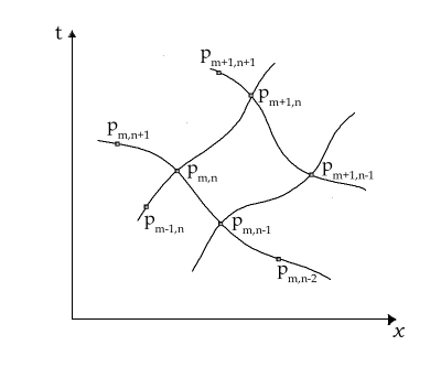
Figure 1:

Figure 2:

Some independence conditions must be imposed on the system (111) e.g.

$$|J|=\left|\frac{\partial(E_{1},\dots,E_{5})}{\partial(x_{m+i_{2},n},t_{m+i_{2}n},x_{m,n+j_{2}},t_{m,n+j_{2}},u_{m+i_{2},n+j_{2}})}\right|\neq 0.$$ (112)

This condition allows us to move upward and to the right along the curves passing through $P_{m,n}$. Moreover, compatibility of the five equations (111) must be assured.

As an example of a P$\Delta$S let us consider the linear heat equation on a uniform and orthogonal lattice. The heat equation in the continuous case is

$$u_{t}=u_{xx}.$$ (113)

An approximation on a uniform orthogonal lattice is given by the five equations

$$E_{1} = \frac{u_{mn+1}-u_{mn}}{h_{2}}-\frac{u_{m+1n}-2u_{mn}+u_{m-1n}}{(h_{1})^{2}}=0$$ (114)

$$E_{2} = x_{m+1,n}-x_{m,n}-h_{1}=0\quad\quad E_{3}=t_{m+1,n}-t_{m,n}=0$$ (115)

$$E_{4} = x_{m,n+1}-x_{mn}=0\quad\quad E_{5}=t_{m,n+1}-t_{m,n}-h_{2}=0.$$ (116)

Equations (115) can of course be integrated to give the standard expressions

$$x_{mn}=h_{1}m+x_{0}\quad t_{mn}=h_{2}n+t_{0}.$$ (117)

Notice that $h_{1}$ and $h_{2}$ are constants that cannot be scaled (they are fixed in eq. (115). On the other hand $(x_{0},t_{0})$ are integration constants and are thus not fixed by the system (115), (116). As written, these equations are invariant under translations, but not under dilations.

Finally, we remark that the usual fixed lattice condition is obtained from (116) by putting $x_{0}=t_{0}=0$, $h_{1}=h_{2}=1$ and identifying

$$x=m,\quad t=n.$$ (118)

Though the above example is essentially trivial, it brings out several points.

1. Four equations are indeed needed to specify a two-dimensional lattice and to allow us to move along the coordinate lines.

2. In order to solve the P$\Delta$S (114), (115) for $h_{1}$ and $h_{2}$ given, we must specify for instance $\{x_{mn},t_{mn},u_{mn},u_{m+1,n},u_{m-1n}\}$. Then we can directly calculate $\{x_{m+1,n},t_{m+1n}\}$, $\{x_{mn+1},t_{m,n+1}\}$ from eq. (115). In order to calculate the coordinates of the fourth point figuring in eq. (114), namely $\{x_{mn-1},t_{m,n-1}\}$ we must shift eq. (115) down by one unit in $m$.

3. The Jacobian condition (112) allowing us to perform these calculations, is obviously satisfied, since we have

   $$\left|\frac{\partial(E_{1},E_{2},E_{3},E_{4},E_{5})}{\partial(x_{m+1,n},t_{m+1,n},x_{m,n+1},t_{mn+1},u_{mn+1})}\right|=1.$$ (119)

A partial difference scheme with one dependent and $n$ independent variables will involve $n^{2}+1$ relations between the variables $(x_{1},x_{2},\dots x_{n},u)$, evaluated at a finite number of points.

3.2 Symmetries of Partial Difference Schemes

As in the case of O$\Delta$S treated in Chapter 2, we shall restrict ourselves to point transformations

$$\tilde{x}=F_{\lambda}(x,t,u)\quad\tilde{t}=G_{\lambda}(x,t,u),\quad\tilde{u}=H_{\lambda}(x,t,u).$$ (120)

The requirement is that $\tilde{u}_{\lambda}(\tilde{x},\tilde{t})$ should be a solution, whenever it is defined and whenever $u(x,t)$ is a solution. The group action (120) should be defined and invertible, at least locally, in some neighbourhood of the reference point $P_{mn}$, including all points $P_{m+i,n+j}$ involved in the system (111).

As in the case of a single independent variable we shall consider infinitesimal transformations that allow us to use Lie algebraic techniques. Instead of transformations (120) we consider

$$\tilde{x} = x+\lambda\xi(x,t,u),$$

$$\tilde{t} = t+\lambda\tau(x,t,u),$$ (121)

$$\tilde{u} = u+\lambda\phi(x,t,u)\quad|\lambda|<<1.$$

Once the functions $\xi$, $\tau$ and $\phi$ are determined from the invariance requirement, then the actual transformations (120) are determined by integration, as in eq. (5), (6).

The transformations act on the entire space $(x,t,u)$, at least locally. This means that the same function $F$, $G$ and $H$ in eq. (120), or $\xi$, $\tau$ and $\phi$ in eq. (121) determine the transformations of all points.

We formulate the problem of determining the symmetries (121), and ultimately (120), in terms of a Lie algebra of vector fields of the form

$$\widehat{X}=\xi(x,t,u)\partial x+\tau(x,t,u)\partial_{t}+\phi(x,t,u)\partial_{u},$$ (122)

where $\xi$, $\tau$ and $\phi$ are the same as in eq. (121). The operator (122) acts at one point only, namely $(x,t,u)\equiv(x_{mn},t_{mn},u_{mn})$. Its prolongation will act at all points figuring in the system(111) and we put

$$\mathop{\mathrm{pr}}\nolimits X=\sum_{j,k}[\xi(x_{jk},t_{jk},u_{jk})\partial_{x_{jk}}+\tau(x_{jk},t_{jk},u_{jk})\partial_{t_{jk}}$$

$$+\phi(x_{jk},t_{jk},u_{jk})\partial_{u_{jk}}],$$

where the sum is over all points figuring in eq. (111). To simplify notation we put

$$\xi_{jk} \equiv \xi(x_{jk},t_{jk},u_{jk}),\quad\tau_{jk}\equiv\tau(x_{jk},t_{jk},u_{jk})$$ (124)

$$\phi_{jk} \equiv \phi(x_{jk},t_{jk},u_{jk}).$$

The functions $\xi$, $\tau$, and $\phi$ figuring in eq. (122) and (3.2) are determined from the invariance condition

$$\mathop{\mathrm{pr}}\nolimits\widehat{X}E_{a}\mid_{E_{1}=\dots=E_{5}=0}=0\quad a=1,\dots 5.$$ (125)

It is eq. (125) that provides an algorithm for determining the symmetry algebra, i.e. the coefficients $\xi$, $\tau$ and $\phi$.

The procedure is the same as in the case of ordinary difference schemes, described in Chapter 2. In the case of the system (111), we proceed as follows:

1. Choose 5 variables $v_{a}$ to eliminate from the condition (125) and express them in terms of the other variables, using the system (111) and the Jacobian condition (112). For instance, we can choose

   $$v_{1} = x_{m+i_{2},n},\quad v_{2}=t_{m+i_{2},n}$$ (126)

   $$v_{3} = x_{m,n+j_{2}},\quad v_{4}=t_{m,n+j_{2}},\quad v_{5}=u_{m+i_{2},j+i_{2}}$$

   and use (111) to express

   $$\begin{array}[]{c}v_{a}=v_{a}(x_{m+i,n+j},t_{m+i,n+j},u_{m+i,n+j})\\[3.0pt] i_{1}\leq i\leq i_{2}-1,\quad j_{1}\leq j\leq j_{2}-1.\end{array}$$

   The quanties $v_{a}$ must be chosen consistently. None of them can be a shifted value of another one (in the same direction). No relations between the quantities $v_{a}$ should follow from the system (111). Once eliminated from eq. (124), they should not reappear due to shifts. For instance, the choice (126) is consistent if $m+i_{2}$ and $n+j_{2}$ are the highest values of these labels that figure in eq. (111).

2. Once the quantities $v_{a}$ are eliminated from the system (125), using (1.), each remaining value of $x_{i,k}$, $t_{i,k}$ and $u_{i,k}$ is independent. Each of them can figure in the corresponding functions $\xi_{ik}$, $\tau_{ik}$, $\phi_{ik}$ (see eq. (124)), in the functions $E_{a}$ directly, or via the expressions $v_{a}$, in the functions $\xi$, $\tau$ and $\phi$ with different labels. This provides a system of five functional equations for $\xi$, $\tau$ and $\phi$.

3. Assume that the dependence of $\xi$, $\tau$ and $\phi$ on $x$, $t$ and $u$ is analytic. Convert the obtained functional equations into differential equations by differentiating with respect to $x_{ik}$, $t_{ik}$, or $u_{ik}$. This provides an overdetermined system of differential equations that we must solve. If possible, use multiple differentiations to obtain single term differential equations that are easy to solve.

4. Substitute the solution of the differential equations back into the original functional equations and solve these. The differential equations are consequences of the functional ones and will hence have more solutions. The functional equations will provide further restrictions on the constants and arbitrary functions obtained when integrating the differential consequences.

   Let us now consider examples on different lattices.

3.3 The Discrete Heat Equation

3.3.1 The Continuous Heat Equation

The symmetry group of the continuous heat equation (113) is well known [48]. Its symmetry algebra has the structure of a semidirect sum

$$L=L_{0}\mathbin{\hbox to0.0pt{\raisebox{0.3pt}{\small$+$}\hss}\mskip-4.0mu\supset}L_{1},$$ (127)

where $L_{0}$ is six-dimensional and $L_{1}$ is an infinite dimensional ideal representing the linear superposition principle (present for any linear PDE). A convenient basis for this algebra is given by the vector fields

$$P_{0} = \partial_{t},\quad D=4t\partial_{t}+2x\partial_{x}+u\partial_{u}$$

$$K = 4t(t\partial_{t}+x\partial_{x})+(x^{2}+2t)u\partial_{u}$$ (128)

$$P_{1} = \partial_{x},B=2t\partial_{x}+xu\partial_{u},\quad W=u\partial_{u}$$

$$S = S(x,t)\partial_{u},\quad S_{t}-S_{xx}=0.$$ (129)

The $\mathop{\mathrm{sl}}(2,\mathbf{R})$ subalgebra $\{P_{0},D,K\}$ represents time translations, dilations and “expansions”. The Heisenberg subalgebra $\{P_{1},B,W\}$ represents space translations, Galilei boosts and the possibility of multiplying a solution $u$ by a constant. The presence of $\widehat{S}$ simply tells us that we can add a solution to any given solution. Thus, $\widehat{S}$ and $\widehat{W}$ reflect linearity, $\widehat{P}_{0}$ and $\widehat{P}_{1}$ the fact that the equation is autonomous (constant coefficients).

3.3.2 Discrete Heat Equation on Fixed Rectangular Lattice

Let us consider the discrete heat equation (114) on the four point uniform orthogonal lattice (115), (116). We apply the prolonged operator (113) to the equations for the lattice and obtain

$$\begin{array}[]{c}\xi(x_{m+1n},t_{m+1n},u_{m+1n})-\xi(x_{mn},t_{mn},u_{mn})=0\\[3.0pt] \xi(x_{m,n+1},t_{m,n+1},u_{m,n+1})-\xi(x_{mn},t_{mn},u_{mn})=0\end{array}$$ (130)

and similarly for $\tau(x,t,u)$. The quantities $v_{i}$ of eq. (126) can be chosen to be

$$\begin{array}[]{c}v_{1}=x_{m+1,n}\quad v_{2}=t_{m+1,n}\quad v_{3}=x_{m,n+1},\\[3.0pt] v_{4}=t_{m,n+1},\quad v_{5}=u_{m,n+1}.\end{array}$$ (131)

However, in (130) $u_{m+1,n}$ and $u_{m,n+1}$ cannot be expressed in terms of $u_{mn}$, since eq. (114) also involves $u_{m-1,n}$. Differentiating (130) with respect to e.g. $u_{mn}$. we find that $\xi$ cannot depend on $u$:

$$\frac{\partial\xi(x_{mn},t_{mn},u_{mn})}{\partial u_{mn}}=0.$$ (132)

Since we have $t_{n+1n}=t_{mn}$ and $x_{mn+1}=x_{mn}$ the two equations (130) yield

$$\frac{\partial\xi_{mn}}{\partial x_{mn}}=0,\quad\frac{\partial\xi_{mn}}{\partial t_{mn}}=0,$$ (133)

respectively. The same is obtained for the coefficient $\tau$, so finally we have

$$\xi=\xi_{0},\quad\tau=\tau_{0},$$ (134)

where $\xi_{0}$ and $\tau_{0}$ are constants.

Now let us apply $\mathop{\mathrm{pr}}\nolimits X$ to eq. (114). We obtain

$$\phi_{mn+1}-\phi_{mn}-\frac{h_{2}}{(h_{1})^{2}}(\phi_{m+1n}-2\phi_{mn}+\phi_{m-1,n})=0.$$ (135)

In more detail, eliminating the quantities $v_{a}$ in eq (131) we have

$$\phi\left(x_{mn},t_{mn}+h_{2},u_{m,n}+\frac{h_{2}}{h^{2}_{1}}(u_{m+1,n}-2u_{m,n}+u_{m-1,n})\right)$$ (136)

$$-\phi(x_{m,n},t_{m,n},u_{m,n})-\frac{h_{2}}{h^{2}_{1}}[\phi(x_{mn}+h_{1},t_{mn},u_{m+1,n})-2\phi(x_{m,n},t_{m,n},u_{m,n})$$

$$\hskip 144.54pt+\phi(x_{mn}-h_{1},t_{mn},u_{m-1,n})]=0.$$

We differentiate eq. (136) twice, with respect to $u_{m+1,n}$ and $u_{m-1,n}$ respectively. We obtain

$$\frac{\partial^{2}\phi_{mn+1}}{\partial u_{m,n+1}^{2}}=0,$$ (137)

that is

$$\phi_{mn}=A(x_{mn},t_{m,n})u_{mn}+B(x_{m,n},t_{m,n}).$$ (138)

We substitute $\phi_{mn}$ of eq. (138) back into eq. (136) and set the coefficients of $u_{m+1,n}$, $u_{mn}$, $u_{m-1n}$ and 1 equal to zero separately. From the resulting determining equations we find that $A(x_{mn},t_{mn})=A_{0}$ must be constant and that $B(x,t)$ must satisfy the discrete heat equation (114). The result is that the symmetry algebra of the system (114) - (116) is very restricted. It is generated by

$$P_{0}=\partial_{t},\quad P_{1}=\partial_{x},\quad W=u\partial_{u},\quad S=S(x,t)\partial_{u}$$ (139)

and reflects only the linearity of the system and the fact that it is autonomous.

The dilations, expansions and Galilei boosts, generated by $D$, $K$ and $B$ of eq. (128) in the continuous case are absent on the lattice (115) and (116). Other lattices will allow other symmetries.

3.3.3 Discrete Heat Equation Invariant Under Dilations

Let us now consider a five-point lattice that is also uniform and orthogonal. We put

$$\frac{u_{m,n+1}-u_{m,n}}{t_{m,n+1}-t_{m,n}}=\frac{u_{m+1n}-2u_{m,n}+u_{m-1n}}{(x_{m+1,n}-x_{m,n})^{2}}$$ (140)

$$x_{m+1n}-2x_{mn}+x_{m-1n}=0\quad\quad x_{mn+1}-x_{mn}=0$$ (141)

$$t_{m+1n}-t_{mn}=0\quad\quad t_{m,n+1}-2t_{m,n}+t_{m,n-1}=0.$$ (142)

The variables $v_{a}$ that we shall substitute from eq. (140), (141) and (142) are $x_{m+1,n}$, $t_{m+1,n}$, $x_{m,n+1}$, $t_{m,n+1}$ and $u_{m,n+1}$. Applying $\mathop{\mathrm{pr}}\nolimits X$ to eq. (141) we obtain

$$\xi(2x_{mn}-x_{m-1,n},t_{mn},u_{m+1,n})-2\xi(x_{mn},t_{mn},u_{mn})$$

$$\hskip 112.0187pt+\xi(x_{m-1,n},t_{mn},u_{m-1,n})=0$$ (143)

$$\xi(x_{mn},2t_{m,n}-t_{mn-1},u_{m,n+1})-\xi(x_{mn},t_{mn},u_{mn})=0.$$ (144)

In eq. (144) $u_{mn}$ and $u_{m,n+1}$ are independent. Differentiating with respect to $u_{mn}$ we find $\partial\xi_{mn}/\partial u_{mn}=0$ and hence $\xi$ does not depend on $u$. Differentiating (144) with respect to $t_{mn-1}$ we obtain $\partial\xi_{m,n+1}/\partial t_{m,n+1}=0$. Thus, $\xi$ depends on $x$ alone. Eq. (143) can then be solved and we find that $\xi$ is linear in $x$. Applying $\mathop{\mathrm{pr}}\nolimits X$ to eq. (142) we obtain similar results for $\tau(x,t,u)$. Finally, invariance of the lattice equations (141) and (142) implies:

$$\xi=ax+b,\quad\tau=ct+d.$$ (145)

Let us now apply $\mathop{\mathrm{pr}}\nolimits X$ to eq. (140). We obtain, after using the P$\Delta$S (140) - (142)

$$\frac{\phi_{mn+1}-\phi_{mn}}{t_{m,n+1}-t_{m,n}}-\frac{\phi_{m+1n}-2\phi_{mn}+\phi_{m-1n}}{(x_{m+1,n}-x_{m,n})^{2}}$$

$$\hskip 86.72377pt+(2a-c)\frac{u_{m+1,n}-2u_{mn}+u_{m-1,n}}{(x_{m+1n}-x_{mn})^{2}}=0.$$ (146)

Notice that $u_{m,n+1}$ (and hence $\phi_{m,n+1}$) depends on $u_{m+1,n}$ and $u_{m-1,n}$, whereas all terms in eq. (146) depend on at most one of these quantities. Taking the second derivative $\partial u_{m+1,n}\partial u_{m-1,n}$ of eq. (146), we find

$$\frac{\partial^{2}\phi_{m,n+1}}{\partial u_{m,n+1}}=0,\mbox{ i.e. }\phi=A(x,t)u+B(x,t).$$ (147)

We substitute this expression back into (146) and find

$$A(x,t)=A_{0}=\mathop{\mathrm{const}}$$ (148)

and see that $B(x,t)$ must satisfy the system (140)–(142). Moreover, we find $c=2a$ in eq. (145). Finally, the symmetry algebra has the basis

$$P_{0} = \partial_{t},\quad P_{1}=\partial_{x},\quad W=u\partial_{u},\quad D=x\partial_{x}+2t\partial_{t}$$ (149)

$$S = S(x,t)\partial u.$$ (150)

Thus, dilational invariance is recovered, not however Galilei invariance. Other symmetries can be recovered on other lattices.

3.4 Lorentz Invariant Difference Schemes

3.4.1 The Continuous Case

Let us consider the PDE

$$u_{xx}-u_{tt}=4f(u).$$ (151)

Eq. (151) is invariant under the Poincaré group of $1+1$ dimensional Minkowski space for any function $f(u)$. Its Lie algebra is represented by

$$P_{0}=\partial_{t},\quad P_{1}=\partial_{x},\quad L=t\partial_{x}+x\partial_{t}.$$ (152)

For specific interactions $f(u)$ the symmetry algebra may be larger, in particular for $f=e^{u}$, $f=u^{N}$, or $f=\alpha u+\beta$.

Before presenting a discrete version of eq. (151), we find it convenient to pass over to light cone coordinates

$$y=x+t,\quad z=x-t$$ (153)

in which eq. (151) is rewritten as

$$u_{yz}=f(u)$$ (154)

and the Poincaré symmetry algebra (152) is

$$P_{1}=\partial_{y},\quad P_{2}=\partial_{z},\quad L=y\partial_{y}-z\partial_{z}.$$ (155)

3.4.2 A Discrete Lorentz Invariant Scheme

A particular P$\Delta$S that has eq. (154) as its continuous limit is

$$\frac{u_{m+1n+1}-u_{mn+1}-u_{m+1n}+u_{mn}}{(y_{m+1n}-y_{mn})(z_{mn+1}-z_{mn})}=f(u_{mn})$$ (156)

$$y_{m+1n}-2y_{mn}+y_{m-1n}=0\quad y_{mn+1}-y_{mn}=0$$ (157)

$$z_{m+1n}-z_{mn}=0\quad z_{mn+1}-2z_{mn}+z_{mn-1}=0.$$ (158)

To find the Lie point symmetries of this difference scheme, we put

$$X=\eta(y,z,u)\partial_{y}+\xi(y,z,u)\partial_{z}+\phi(y,z,u)\partial_{u}.$$ (159)

We apply the prolonged vector field $\mathop{\mathrm{pr}}\nolimits\widehat{x}$ first to eq. (157) and (158), eliminate $y_{m+1n}$, $y_{m,n+1}$, $z_{m+1n}$ and $z_{m,n+1}$, using the system (157), (158) and notice that all $u_{ik}$ that figure in the obtained equations for $\eta_{ik}$ and $\xi_{ik}$ are independent.

The result that we obtain is that $\eta$ and $\xi$ must be independent of $u$ and linear in $y$ and $z$, respectively. Finally we obtain

$$\xi=\alpha y+\gamma,\quad\eta=\beta z+\delta$$ (160)

($\alpha,\dots,\delta$ are constants). Invariance of eq. (156) implies that the coefficient $\phi$ in the vector field (159) must be linear in $u$ and moreover have the form

$$\phi=Au+B(y,z)$$ (161)

where $A$ is a constant. Taking (160) and (161) into account and applying $\mathop{\mathrm{pr}}\nolimits X$ to eq. (156), we obtain

$$(A-\alpha-\beta)f(u_{mn})+\frac{B_{m+1n+1}-B_{mn+1}-B_{m+1n}+B_{mn}}{(y_{m+1,n}-y_{mn})(z_{mn+1}-z_{mn})}$$

$$=(Au_{mn}+B_{mn})f^{\prime}(u_{mn}).$$ (162)

Differentiating eq. (162) with respect to $u_{mn}$ we finally obtain the following determining equation:

$$(\alpha+\beta)\frac{df}{du_{mn}}+[Au_{mn}+B(y_{mn},z_{mn})]\frac{d^{2}f}{du_{mn}^{2}}=0.$$ (163)

For $f(u_{mn})$ arbitrary, we find $\beta=-\alpha$, $A=B=0$. Thus for arbitrary $f(u)$ the scheme (156)–(157) has the same symmetries as its continuous limit. The point symmetry algebra is given by eq.  (155), i.e. it generates, translations and Lorentz transformations.

Now let us find special cases of $f(u)$ when further symmetries exist. That means that eq. (163) must be solved in a nontrivial manner. Let us restrict ourselves to the case when the interaction is nonlinear, i.e.

$$\frac{d^{2}}{du_{mn}^{2}}f(u_{m,n})\neq 0.$$ (164)

Then we must have

$$B(y_{mn},z_{mn})=B=\mathop{\mathrm{const}}.$$ (165)

The equation to be solved for $f(u)$ is actually eq. (162) which simplifies to

$$(Au+B)f^{\prime}(u)=(A-\alpha-\beta)f(u).$$ (166)

For $A\neq 0$ the solution of eq. (166) is

$$f=f_{0}u^{p}$$ (167)

and the symmetry is

$$D_{1}=y\partial_{y}+z\partial_{z}-\frac{2}{p-1}u\partial u.$$ (168)

For $A=0$, $B\neq 0$ we obtain

$$f=f_{0}e^{pu}$$ (169)

and the additional symmetry is

$$D_{2}=y\partial_{y}+z\partial_{z}-2\partial_{u}.$$ (170)

Thus, for nonlinear interactions $f(u)$, $f^{\prime\prime}\neq 0$, the P$\Delta$S (156)–(158) has exactly the same point symmetries as its continuous limit (154).

The linear case

$$f(u)=Ru+T$$ (171)

is different. The PDE (154) in this case is conformally invariant. This infinite dimensional symmetry algebra is not present for the discrete case considered in this section.

4 Symmetries of Discrete Dynamical Systems

4.1 General Formalism

In this chapter we shall discuss differential-difference equations on a fixed one-dimensional lattice. Thus, time $t$ will be a continuous variable, $n\in\mathbf{Z}$ a discrete one. We will be modeling discrete monoatomic or diatomic molecular chains with equally spaced rest positions. The individual atoms will be vibrating around their rest positions. For monoatomic chains the actual position of the $n$-th atom is described by one continuous variable $u_{n}(t)$. For diatomic atoms there will be two such functions, $u_{n}(t)$ and $v_{n}(t)$.

Only nearest neighbour interaction will be considered. The interaction are described by a priori unspecified functions. Our aim is to classify these functions according to their symmetries.

Three different models have been studied [42, 23, 34]. They correspond to Fig. 3, 4 and 5, respectively.

The model illustrated on Fig. 3 corresponds to the equation [42]

$$\ddot{u}_{n}(t)-F_{n}\big{(}t,u_{n-1}(t),u_{n}(t),u_{n+1}(t)\big{)}=0.$$ (172)

Fig. 4 could correspond to a very primitive model of the DNA molecule. The equations are [23]

$$\ddot{u}_{n} = F_{n}\big{(}t,u_{n-1}(t),u_{n}(t),u_{n+1}(t),v_{n-1}(t),v_{n}(t),v_{n+1}(t)\big{)}=0$$

$$\ddot{v}_{n} = G_{n}\big{(}t,u_{n-1}(t),u_{n}(t),u_{n+1}(t),v_{n-1}(t),v_{n}(t),v_{n+1}(t)\big{)}=0.$$ (173)

The model corresponding to Fig. 5 already took translational and Galilei invariance into account, so the equations were

$$\ddot{u}_{n} = F_{n}(\xi_{n},t)+G_{n}(\eta_{n-1},t)$$

$$\ddot{v}_{n} = K_{n}(\xi_{n},t)+P_{n}(\eta_{n-1},t)$$ (174)

$$\xi_{n} = y_{n}-x_{n},\quad\eta_{n}=x_{n+1}-y_{n}.$$

Figure 3: A monoatomic chain

Figure 4: A diatomic molecule with two types of atoms on parallel chains

Figure 5: A diatomic molecule with two types of atoms alternating along one chain

Dissipation was ignored in all three cases, so no first derivatives are present.

In these lectures we shall only treat the case (172). The lattice is fixed, i.e. it is given by the relation

$$x_{n}=hn+x_{0}$$ (175)

with $h$ and $x_{0}$ given constants. With no loss of generality we can choose $h=1$, $x_{0}=0$, so that we have $x_{n}=n$.

Our aim is to find all functions $F_{n}$ for which eq. (172) allows a nontrivial group of local Lie point transformations. We shall also assume that the interaction is nonlinear and that it does indeed couple neighbouring states.

Let us sum up the conditions imposed on the model (172) and on the symmetry studies.

1. The lattice is fixed and regular $(x_{n}=n)$.

2. The interaction involves nearest neighbours only, is nonlinear and coupled, i.e.

   $$\frac{\partial^{2}F_{n}}{\partial u_{i}\partial u_{k}}\neq 0,\quad\frac{\partial F_{n}}{\partial u_{n-1}}\neq 0,\quad\frac{\partial F_{n}}{\partial u_{n+1}}\neq 0.$$ (176)

3. We consider point symmetries only. Since the lattice is fixed, the transformations are generated by vector fields of the form [38]

   $$\widehat{X}=\tau(t)\partial_{t}+\phi_{n}(t,u_{n})\partial u_{n}.$$ (177)

   We also assume that $\tau(t)$ is an analytical function of $t$ and $\phi_{n}(t,u_{n})$ is also analytic as a function of $t$ and $u_{n}$.

The symmetry algorithm is the usual one, namely

$$\mathop{\mathrm{pr}}\nolimits\widehat{X}E_{n}\mid_{E_{n}=0}=0.$$ (178)

The prolongation in eq. (178) involves a prolongation to $t$-derivatives $\dot{u}_{n}$ and $\ddot{u}_{n}$, and to all values of $n$ figuring in eq. (172), i.e. $n\pm 1$.

The terms in the prolongation that we actually need are

$$\mathop{\mathrm{pr}}\nolimits^{(2)}X=\tau\partial_{t}+\sum^{n+1}_{k=n-1}\phi_{k}(t,u_{k})\partial_{u_{k}}+\phi^{tt}_{n}\partial_{\ddot{u}_{n}}.$$ (179)

The coefficient $\phi^{tt}_{n}$ is calculated using the formulas of Chapter 1 (or e.g. Ref. [48]). We have

$$\phi^{tt}_{n}=D^{2}_{t}\phi_{n}-(D^{2}_{t}\tau)u_{n}-2(D_{t}\tau)\ddot{u}_{n}.$$ (180)

Applying $\mathop{\mathrm{pr}}\nolimits^{(2)}X$ to eq. (172) and replacing $\ddot{u}$ from that equation, we get an expression involving $(\dot{u}_{n})^{3}$, $(\dot{u}_{n})^{2}$, $(\dot{u}_{n})^{1}$ and $(\dot{u}_{n})^{0}$. The coefficients of all of these terms must vanish separately. The first three of these equations do not depend on $F_{n}$ and can be solved easily. They imply

$$\phi_{n}(t,u_{n})=\left(\frac{1}{2}\dot{\tau}(t)+a_{n}\right)u_{n}+\beta_{n}(t),\quad\tau=\tau(t),\quad\dot{a}_{n}=0.$$ (181)

The remaining determining equation is

$$\frac{1}{2}\tau_{ttt}u_{n}+\ddot{\beta}_{n}+\left(a_{n}+\frac{3}{2}\dot{\tau}\right)F_{n}$$ (182)

$$\hskip 36.135pt-\tau F_{n,t}-\sum_{\alpha}\left[\left(\frac{1}{2}\dot{\tau}+a_{\alpha}\right)u_{\alpha}+\beta_{\alpha}\right]F_{n,u_{\alpha}}=0,$$

and the vector fields realizing the symmetry algebra are

$$\widehat{X}=\tau(t)\partial_{t}+\left[\left(\frac{1}{2}\dot{\tau}(t)+a_{n}\right)u_{n}+\beta_{n}(t)\right]\partial u_{n}.$$ (183)

Since we are classifying the interactions $F_{n}$, we must decide which functions $F_{n}$ will be considered to be equivalent. To do this we introduce a group of “allowed transformations”, or a “classifying group”. We define this to be a group of fiber preserving point transformations

$$u_{n}(t)=\Omega_{n}(\tilde{u}_{n}(\tilde{t}),\tilde{t},g),\quad\tilde{t}=\tilde{t}(t,g),\quad\tilde{n}=n,$$ (184)

taking eq. (172) into an equation of the same form

$$\ddot{\tilde{u}}_{n}(\tilde{t})=\tilde{F}_{n}\big{(}\tilde{t},\tilde{u}_{n-1}(\tilde{t}),\tilde{u}_{n}(\tilde{t}),\tilde{u}_{n+1}(\tilde{t})\big{)}=0.$$ (185)

That is, the allowed transformations can change the function $F_{n}$ (as opposed to symmetry transformations), but cannot introduce first derivatives, nor other than nearest neighbour terms. These conditions narrow down the transformations (184) to linear ones of the form

$$u_{n}(t) = \frac{A_{n}}{\sqrt{\tilde{t}_{t}}}\tilde{u}_{n}(\tilde{t})+B_{n}(t),\quad\tilde{t}=\tilde{t}(t)$$

$$A_{n,t} = 0,\quad\tilde{t}_{t}\neq 0,\quad A_{n}\neq 0,\quad\tilde{n}=n.$$ (186)

Eq. (172) is transformed into

$$\tilde{u}_{n,\tilde{t}\tilde{t}}=A^{-1}_{n}(\tilde{t}_{t})^{-3/2}\biggl{\{}F_{n}(t,u_{n-1},u_{n},u_{n+1})$$ (187)

$$\quad\quad+\biggl{[}-\frac{3}{4}A_{n}(\tilde{t}_{t})^{-5/2}(\tilde{t}_{tt})^{2}$$

$$\qquad\qquad\qquad+\frac{A_{n}}{2}(\tilde{t}_{t})^{-3/2}\tilde{t}_{ttt}\biggr{]}\tilde{u}_{n}(\tilde{t})-B_{n,tt}\biggr{\}}.$$

The transformed vector field (183) is

$$\widehat{X}=\tau(t)\tilde{t}_{t}(t)\partial_{\tilde{t}}+\left\{\left[\frac{1}{2}\big{(}\tau(t)\tilde{t}_{t}\big{)}_{\tilde{t}}+a_{n}\right]\tilde{u}_{n}\right\}$$ (188)

$$+\left.(\tilde{t}_{t})^{1/2}A^{-1}_{n}\left[\left(\frac{1}{2}\tau_{t}+a_{n}\right)B_{n}+\beta_{n}-\tau B_{n,t}\right]\right\}\partial\tilde{u}_{n}.$$

In eq. (187) and (188) $\tau(t)$, $a_{n}$, $\beta_{n}$ and $F_{n}$ are given, whereas $\tilde{t}(t)$, $A_{n}$ and $B_{n}(t)$ are ours to choose. We use these quantities to simplify the vector field $\widehat{X}$.

Our classification strategy is the following one. We first classify one-dimensional subalgebras. Thus, we have one vector field of the form (183). If $\tau(t)$ satisfies $\tau(t)\neq 0$ in some open interval, we use $\tilde{t}(t)$ to normalize $\tau(t)=1$ and $B_{n}(t)$ to transform $\beta_{n}(t)$ into $\beta_{n}(t)=0$. If we have $\tau(t)=0$, $a_{n}\neq 0$, we use $B_{n}(t)$ to annul $\beta_{n}(t)$. The last possibility is $\tau(t)=0$, $a_{n}=0$, $\beta_{n}(t)\neq 0$. Then we cannot simplify further. The same transformations will also simplify the determining equation (182) and we can, in each case, solve it for the interaction $F_{n}(t,u_{n-1},u_{n},u_{n+1})$.

Once all interactions allowing one dimensional symmetry algebras are determined, we proceed further structurally. We first find all Abelian symmetry groups and the corresponding interactions allowing them. We run through our list of one-dimensional algebras and take them in an already establlished “canonical” form. Let us call this element $X_{1}$ (in each case). We then find all elements $X$ of the form (183) that satisfy $[X_{1},X]=0$. We classify the obtained operators $X$ under the action of a subgroup of the group of allowed transformations, namely the isotropy group of $X_{1}$ (the group that leaves the subalgebra $X_{1}$ invariant). For each Abelian group we find the invariant interaction.

¿From Abelian symmetry algebras we proceed to nilpotent ones, then to solvable ones and finally to nonsolvable ones. These can be semisimple, or they may have a nontrivial Levi decomposition.

All details can be found in the original article [42], here we shall present the main results.

4.2 One-Dimensional Symmetry Algebras

Three classes of one-dimensional symmetry algebras exist. Together with their invariant interactions, they can be represented by

$$A_{1,1}\qquad X=\partial_{t}+a_{n}u_{n}\partial u_{n}$$

$$F_{n}(t,u_{k})=f_{n}(\xi_{n-1},\xi_{n},\xi_{n+1})e^{a_{n}t}$$

$$\xi_{k}=u_{k}e^{-a_{k}t},\quad k=n-1,n,n+1.$$

$$A_{1,2}\qquad X=a_{n}u_{n}\partial u_{n}$$

$$F_{n}(t,u_{k})=u_{n}f_{n}(t,\xi_{n-1},\xi_{n+1})$$

$$\xi_{n\pm 1}=u^{a_{n}}_{n\pm 1}u^{a_{n\pm 1}}_{n}.$$

$$A_{1,3}\qquad X=\beta_{n}(t)\partial u_{n}$$ (191)

$$F_{n}(t,u_{k})=\frac{\ddot{\beta}_{n}}{\beta_{n}}u_{n}+f_{n}(t,\xi_{n-1},\xi_{n+1})$$

$$\xi_{n\pm 1}=\beta_{n}(t)u_{n\pm 1}-\beta_{n\pm 1}(t)u_{n}.$$

We see that the existence of a one-dimensional Lie algebra implies that the interaction $F$ is an arbitrary function of three variables, rather than the original four. The actual form of the interaction in eq. (4.2), (4.2) and (191) was obtained by solving eq. (182), once the canonical form of vector field $X$ in eq. (4.2), (4.2), or (191) was taken into account.

4.3 Abelian Lie Algebras of Dimension $N\geq 2$

Without proof we state several theorems.

Theorem 1.

An Abelian symmetry algebra of eq. (172) can have dimension $N$ satisfying $1\leq N\leq 4$.

Comment: For $N=1$ these are the algebras $A_{1,1}$, $A_{1,2}$ and $A_{1,3}$ of eq. (4.2), (4.2) and (191).

Theorem 2.

Five distinct classes of interactions $F_{n}$ exist having symmetry algebras of dimension $N=2$. For four of them the interaction will involve an arbitrary function of two variables, for the fifth $a$ function of three variables.

The five classes can be represented by the following algebras and interactions.

$$A_{2,1}:\quad X_{1}=\partial_{t}+a_{1n}u_{n}\partial u_{n},\quad X_{2}=a_{2n}u_{n}\partial u_{n}$$

$$F_{n}=u_{n}f_{n}(\xi_{n-1},\xi_{n+1}),\quad a_{2n}\neq 0$$

$$\xi_{k}=u^{a_{2n}}_{k}u^{-a_{2k}}_{n}e^{(a_{1n}a_{2k}-a_{1k}a_{2n})t},\qquad k=n\pm 1$$

$$A_{2,2}:\quad X_{1}=\partial_{t}+a_{n}u_{n}\partial u_{n}\quad X_{2}=e^{a_{n}t}\partial u_{n}$$

$$F_{n}=a^{2}_{n}u_{n}+e^{a_{n}t}f_{n}(\xi_{n-1},\xi_{n+1})$$

$$\xi_{k}=u_{k}e^{-a_{k}t}-u_{n}e^{-a_{n}t},\quad k=n\pm 1$$

$$A_{2,3}:\quad X_{1}=a_{1n}u_{n}\partial u_{n}\quad X_{2}=a_{2n}u_{n}\partial u_{n}$$

$$F_{n}=u_{n}f_{n}(t,\xi)$$

$$\xi=u^{\alpha_{n+1,n}}_{n-1}u^{\alpha_{n-1,n+1}}_{n}u^{\alpha_{n,n-1}}_{n+1}$$

$$\alpha_{kl}=a_{1k}a_{2l}-a_{1l}a_{2k}\neq 0$$

$$A_{2,4}:\quad X_{1}=\beta_{1,n}(t)\partial u_{n},\quad X_{2}=\beta_{2n}(t)\partial u_{n}$$

$$\quad\quad\quad\beta_{1n}\beta_{2n+1}-\beta_{1n+1}\beta_{2n}\neq 0$$

$$F_{n}=\frac{(\beta_{1n}\ddot{\beta}_{2n}-\ddot{\beta}_{1n}\beta_{2n})u_{n+1}-(\beta_{1n+1}\ddot{\beta}_{2n}-\ddot{\beta}_{1n}\beta_{2n+1})}{\beta_{1n}\beta_{2n+1}-\beta_{1n+1}\beta_{2n}}$$

$$\quad\quad\quad+f_{n}(t,\xi)$$

$$\xi=(\beta_{1n}\beta_{2n+1}-\beta_{1n+1}\beta_{2n})u_{n-1}+(\beta_{1n+1}\beta_{2n-1}-\beta_{1n-1}\beta_{2n+1})u_{n}$$

$$\quad\quad\quad+(\beta_{1n-1}\beta_{2n}-\beta_{1n}\beta_{2n-1})u_{n+1}$$

$$A_{2,5}:\quad X_{1}=\partial u_{n},\quad X_{2}=t\partial u_{n}$$ (196)

$$F_{n}=f_{n}(t,\xi_{n-1},\xi_{n+1}),\quad\xi_{k}=u_{k}-u_{n},\quad k=n\pm 1$$

The algebra $A_{2,5}$ is of particular physical significance since $X_{1}$ and $X_{2}$ in eq. (196) correspond to translation and Galilei invariance for the considered chain. Unless we are considering a molecular chain in some external field, or unless some external geometry is imposed, the symmetry algebra $A_{2,5}$ should always be present, possibly as a subalgebra of a larger symmetry algebra.

Theorem 3.

Precisely four classes of three-dimensional symmetry algebras exist. Only one of them contains the $A_{2,5}$ subalgebra and can be presented as

$$A_{3,4}\quad X_{1}=\partial u_{n},\quad X_{2}=t\partial u_{n},$$ (197)

$$X_{3}=\beta_{n}(t)\partial u_{n},\quad\beta_{n+1}\neq\beta_{n},\,\ddot{\beta}_{n}\neq 0.$$

The invariant interaction is

$$F_{n} = \frac{\ddot{\beta}_{n}}{\beta_{n+1}-\beta_{n}}(u_{n+1}-u_{n})+f_{n}(t,\xi),$$ (198)

$$\xi = (\beta_{n}-\beta_{n+1})u_{n-1}+(\beta_{n+1}-\beta_{n-1})u_{n}+(\beta_{n-1}-\beta_{n})u_{n+1}.$$ (199)

For $A_{3,1}$, $A_{3,2}$ and $A_{3,4}$ see the original article [42].

Theorem 4.

There exist precisely two classes of interactions $F_{n}$ in eq. (172) satisfying conditions (176), allowing four-dimensional symmetry algebras. Only one of them contains the subalgebra $A_{2,5}$ and is represented by the following.

$$A_{4,1}\quad F_{n}=\frac{B_{n}(t)\gamma_{n}}{\gamma_{n}-\gamma_{n+1}}(u_{n}-u_{n+1})+f_{n}(t,\xi),f_{n,\xi\xi}\neq 0$$

$$X_{1}=\partial u_{n},\quad X_{2}=t\partial u_{n},\quad X_{3}=\psi_{1}(t)\gamma_{n}\partial u_{n},$$

$$\quad\quad\quad X_{4}=\psi_{2}(t)\gamma_{n}\partial u_{n}$$

$$\gamma_{n+1}\neq\gamma_{n},\quad\dot{\gamma}_{n}=0,\quad\psi_{1}\dot{\psi}_{2}-\dot{\psi}_{1}\psi_{2}=\mathop{\mathrm{const}}\neq 0$$

with $\xi$ as in eq. (199) and $\psi_{1}$, $\psi_{2}$ satisfying

$$\ddot{\psi}_{i}-B(t)\psi_{i}=0,\quad i=1,2$$

4.4 Some Results on the Structure of Lie Algebras

Let us recall some basic properties of finite-dimensional Lie algebras. Consider a Lie algebra $L\sim\{X_{1},X_{2},\dots,X_{n}\}$, where the elements $X_{i}$ form a basis. To each algebra $L$ one associates two series of subalgebras.

The derived series consist of the algebras

$$L^{0}\equiv L,\quad L^{1}\equiv DL=[L,L],\quad L^{2}\equiv D^{2}L=[DL,DL],\dots$$

$$L^{N}\equiv D^{N}L=[D^{N-1}L,D^{N-1}L].$$ (201)

The algebra of commutators $DL$ is called the derived algebra. If we have $DL=L$, the algebra $L$ is called perfect. If an integer $N$ exists for which we have $D^{N}L=\{0\}$, the algebra $L$ is called solvable.

The central series consist of the algebras

$$L_{0}\equiv L,\quad L_{1}=L^{1}=[L,L],\quad L_{2}=[L,L_{1}],\dots L_{N}=[L,L_{N-1}],\dots$$ (202)

If there exists an integer $N$ for which we have $L_{N}=\{0\}$, the algebra $L$ is called nilpotent. Clearly, every nilpotent algebra is solvable, but the converse is not true.

Let us consider two examples

1. The Lie algebra of the Euclidean group of a plane: $e(2)\sim\{L_{3},P_{1},P_{2}\}$. The commmutation relations are

   $$[L_{3},P_{1}]=P_{2},\quad[L_{3},P_{2}]=-P_{1},\quad[P_{1},P_{2}]=0.$$ (203)

   The derived series is

   $$L=\{L_{3},P_{1},P_{2}\}\supset DL=\{P_{1},P_{2}\},\quad D^{2}L=\{0\}$$

   and the central series is

   $$L\supset L_{1}=\{P_{1},P_{2}\}=L_{2}=L_{3}=\dots$$

   Hence $e(2)$ is solvable but not nilpotent.

2. The Heisenberg algebra $H_{1}\sim\{X_{1},X_{2},X_{3}\}$ where the basis can be reallized e.g. by the derivative operator, the coordinate $x$ and the identity 1:

   $$X_{1}=\partial_{x},X_{2}=x,X_{3}=1.$$

   We have

   $$[X_{1},X_{2}]=X_{3},\quad[X_{1},X_{3}]=[X_{2},X_{3}]=0$$ (204)

   and hence

   $$DL = \{X_{3}\},\quad D^{2}L=0.$$

   $$L_{1} = \{X_{3}\},\quad L_{2}=0.$$

   We see that the Heisenberg algebra is nilpotent (and solvable).

An Abelian Lie algebra is of course also nilpotent.

We shall need some results concerning nilpotent Lie algebras (by nilpotent we mean nilpotent non-Abelian).

1. Nilpotent Lie algebras always contain Abelian ideals.

2. All nilpotent Lie algebras contain the three-dimensional Heisenberg algebra as a subalgebra.

We shall also use some basic properties of solvable Lie algebras, where by solvable we mean solvable, non-nilpotent.

1. Every solvable Lie algebra $L$ contains a unique maximal nilpotent ideal called the nilradical $NR(L)$. The dimension of the nilradical satisfies

   $$\frac{1}{2}\dim(L)\leq\dim NR(L)\leq\dim(L)-1.$$ (205)

2. If the nilradical $NR(L)$ is Abelian, then we can choose a basis for $L$ in the form $\{X_{1},\dots,X_{n},Y_{1},\dots,Y_{m}\},\quad m\leq n$, with commutation relations

   $$[X_{i},X_{k}]=0,\quad[X_{i},Y_{k}]=(A_{k})_{ij}X_{j},\quad[Y_{i},Y_{k}]=C^{l}_{ik}X_{l}.$$ (206)

   The matrices $A_{k}$ commute and are linearly nilindependent (i.e. no linear combination of them is a nilpotent matrix).

If a Lie algebra $L$ is not solvable, it can be simple, semisimple, or it may have a nontrivial Levi decomposition [32]. A simple Lie algebra $L$ has no nontrivial ideals, i.e.

$$I\subseteq L,\quad[I,I]\subseteq I,\quad[L,I]\subseteq I$$ (207)

implies $I\sim\{0\}$, or $I=L$.

A semisimple Lie algebra $L$ is a direct sum of simple Lie algebras $L_{i}$

$$L\sim L_{1}\oplus L_{2}\oplus\dots\oplus L_{p},\quad[L_{i},L_{k}]=0.$$ (208)

If $L$ is not simple, semisimple, or solvable, then it allows a unique Levi decomposition into a semidirect sum

$$L\sim S\mathbin{\hbox to0.0pt{\raisebox{0.3pt}{\small$+$}\hss}\mskip-4.0mu\supset}R,\quad[S,S]=S,\quad[R,R]\subset R,\quad[S,R]\subseteq R$$ (209)

where $S$ is semisimple and $R$ is solvable; $R$ is called the radical of $L$, i.e. the maximal solvable ideal.

Let us now return to the symmetry classification of discrete dynamical systems.

4.5 Nilpotent Non-Abelian Symmetry Algebras

Since every nilpotent Lie algebra contains the three-dimensional Heisenberg algebra, we start by constructing this algebra, $H_{1}\sim\{X_{1},X_{2},X_{3}\}$. The central element $X_{3}$ of eq. (204) is uniquely defined. We start from this element, take it in one of the standard forms (4.2), (4.2), or (191), then construct the two complementary elements $X_{1}$ and $X_{2}$. The result is that two inequivalent realizations of $H_{1}$, exist namely:

$$N_{3,1}:\quad X_{1}=\partial_{u_{n}},\quad X_{2}=\partial_{t},\quad X_{3}=t\partial_{u_{n}}$$ (210)

$$F_{n}=f_{n}(\xi_{n+1},\xi_{n-1}),\quad\xi_{k}=u_{k}-u_{n},\quad k=n\pm 1$$

$$N_{3,2}:\quad X_{1}=e^{a_{n}t}\partial u_{n},\quad X_{2}=\partial_{t}+a_{n}u_{n}\partial u_{n}$$

$$X_{3}=(t+\gamma_{n})e^{a_{n}t}\partial u_{n},\quad\dot{a}_{n}=0,\quad\dot{\gamma}_{n}=0,\gamma_{n+1}\neq\gamma_{n}$$

$$F_{n}=\frac{a^{2}_{n}(\gamma_{n+1}-\gamma_{n})-2a_{n}}{\gamma_{n+1}-\gamma_{n}}u_{n}$$

$$\quad\quad\quad+\frac{2a_{n}}{\gamma_{n+1}-\gamma_{n}}u_{n+1}e^{(a_{n}-a_{n+t})t}+e^{a_{n}t}f_{n}(\xi)$$

$$\xi=(\gamma_{n}-\gamma_{n+1})u_{n-1}e^{-a_{n-1}t}+(\gamma_{n+1}-\gamma_{n-1}),u_{n}e^{-a_{n}t}$$

$$\quad\quad\quad+(\gamma_{n-1}-\gamma_{n})u_{n+1}e^{-a_{n+1}t}.$$

Notice that $N_{3,1}$ contains the physically important subalgebra $A_{2,5}$. whereas $N_{3,2}$ does not.

Extending the algebras $N_{3,1}$ and $N_{3,2}$ by further elements, we find that $N_{3,1}$ gives rise to two five-dimensional nilpotent symmetry algebras $N_{5,k}$ and $N_{3,2}$ to a four-dimensional one $N_{4,1}$.

Here we shall only give $N_{5,1}$ and $N_{5,2}$ which contain $N_{3,1}$ and hence $A_{2,5}$:

$$N_{5,k}:\quad X_{1}=\partial u_{n},\quad X_{2}=t\partial u_{n},\quad X_{3}=\biggl{(}\frac{(k-1)t^{2}}{2}+\gamma_{n}\biggr{)}\partial u_{n},$$

$$X_{4}=\biggl{(}\frac{(k-1)t^{3}}{6}+\gamma_{n}t\biggr{)}\partial u_{n},\quad X_{5}=\partial_{t},\quad k=1,2$$

$$F_{n}=\frac{2(k-1)}{\gamma_{n+1}-\gamma_{n}}(u_{n+1}-u_{n})+f_{n}(\xi)$$

with $\xi$ as in eq. (4.5).

4.6 Solvable Symmetry Algebras with Non-Abelian Nilradicals

We already know all nilpotent symmetry algebras, so we can start from the nilradical and extend it by further non-nilpotent elements. The result can be stated as a Theeorem.

Theorem 5.

Seven classes of solvable symmetry algebras with non-Abelian nilradicals exist for eq. (172). Four of them have $N_{3,1}$ as nilradical, three have $N_{5,1}$.

For $N_{3,1}$ we can add just one further element $Y$, namely one of the following

$$SN_{4,1}:\quad Y=t\partial_{t}+\biggl{(}\frac{1}{2}+a\biggr{)}u_{n}\partial u_{n},\quad a\neq-\frac{1}{2}$$ (213)

$$F_{n}=(u_{n+1}-u_{n})e^{(a-3/2)/(a+1/2)}f_{n}(\xi)$$

$$SN_{4,2}:\quad Y=t\partial_{t}+(2u_{n}+t^{2})\partial u_{n}$$ (214)

$$F_{n}=\ln(u_{n+1}-u_{n})+f_{n}(\xi)$$

$$SN_{4,3}:\quad Y=u_{n}\partial u_{n}$$ (215)

$$F_{n}=(u_{n+1}-u_{n})f_{n}(\xi).$$

In all above cases we have

$$\xi=\frac{u_{n-1}-u_{n}}{u_{n+1}-u_{n}}.$$ (216)

$$SN_{4,4}:\quad Y=t\partial_{t}+\gamma_{n}\partial u_{n},\quad\gamma_{n+1}\neq\gamma_{n},\quad\dot{\gamma}_{n}=0$$ (218)

$$F_{n}=\exp\biggl{(}-2\frac{u_{n+1}-u_{n}}{\gamma_{n+1}-\gamma_{n}}\biggr{)}f_{n}(\xi)$$

$$\xi=(\gamma_{n}-\gamma_{n+1})u_{n-1}+(\gamma_{n+1}-\gamma_{n-1})u_{n}$$

$$\quad\quad\quad+(\gamma_{n-1}-\gamma_{n})u_{n+1}.$$

For $N_{5,1}$ we can also add at most one non-nilpotent element and we obtain

$$SN_{6,1}:\quad Y=t\partial_{t}+\biggl{(}\frac{1}{2}+a\biggr{)}u_{n}\partial u_{n}$$ (219)

$$F_{n}=c_{n}\xi^{(a-3/2)/(a+1/2)},\quad a\neq-\frac{1}{2},\quad a\neq\frac{3}{2}$$

$$SN_{6,2}:\quad Y=t\partial_{t}+[2u_{n}+(a+b\gamma_{n})t^{2}]\partial u_{n},\quad a^{2}+b^{2}\neq 0$$ (220)

$$F_{n}=c_{n}+(a+b\gamma_{n})\ln\xi$$

$$SN_{6,3}:\quad Y=t\partial_{t}+\rho_{n}\partial u_{n},\quad\rho_{n}\neq A+B\gamma_{n},\quad\dot{\rho}_{n}\neq 0$$

$$F_{n}=c_{n}e^{\zeta}$$

$$\xi=\frac{-2\zeta}{(\gamma_{n}-\gamma_{n+1})\rho_{n-1}+(\delta_{n+1}-\gamma_{n-1})\rho_{n}+(\gamma_{n-1}-\gamma_{n})\rho_{n+1}}.$$

In all cases $\xi$ is as in eq. (218).

4.7 Solvable Symmetry Algebras with Abelian Nilradicals

The results in this case are very rich. There exist 31 such symmetry algebras and their dimensions satisfy $2\leq d\leq 5$.

For all details and a full complete list of results we refer to the original article. Here we give just one example of a five-dimensional Lie algebra with $NR(L)=A_{4,1}$.

$$SA_{5,1}:\quad X_{1}=\partial u_{n},\quad X_{2}=t\partial u_{n},\quad X_{3}=e^{t}\gamma_{n}\partial u_{n},$$

$$\quad\quad\quad X_{4}=e^{-t}\gamma_{n}\partial u_{n}$$

$$Y=\partial_{t}+au_{n}\partial u_{n}\quad a\neq 0,\quad\gamma_{n}\neq\gamma_{n+1},\quad\dot{\gamma}_{n}=0$$

$$F_{n}=\frac{\gamma_{n}(u_{n+1}-u_{n})}{\gamma_{n+1}-\gamma_{n}}+e^{at}f_{n}(\xi)$$

$$\xi=[(\gamma_{n}-\gamma_{n+1})u_{n-1}+(\gamma_{n+1}-\gamma_{n-1})u_{n}$$

$$\quad\quad\quad+(\gamma_{n-1}-\gamma_{n})u_{n+1}]e^{-at}.$$

4.8 Nonsolvable Symmetry Algebras

A Lie algebra that is not solvable must have simple subalgebra. The only simple algebra that can be constructed out of vector fields of the form (183) is $\mathop{\mathrm{sl}}(2,\mathbf{R})$. The algebra and the corresponding invariant interaction can be represented as:

$$NS_{3,1}:\quad X_{1}=\partial_{t},\quad X_{2}=t\partial_{t}+\frac{1}{2}u_{n}\partial u_{n}$$

$$X_{3}=t^{2}\partial_{t}+tu_{n}\partial u_{n}$$

$$F_{n}=\frac{1}{u^{3}_{n}}f_{n}(\xi_{n-1},\xi_{n+1}),\quad\xi_{k}=\frac{u_{k}}{u_{n}}.$$

This algebra can be further extended to a four, five or seven-dimensional symmetry algebra. In two cases the algebra will have an $A_{2,5}$ subalgebra, namely

$NS_{5,1}$: In addition to $X_{1}$, $X_{2}$, $X_{3}$ of (4.7) we have

$$X_{4} = \partial u_{n},\quad X_{5}=t\partial u_{n}$$

$$F_{n} = (u_{n+1}-u_{n})^{-3}f_{n}(\xi),\quad\xi=\frac{u_{n+1}-u_{n}}{u_{n-1}-u_{n}}.$$ (224)

$NS_{7,1}$: The additional elements are

$$\begin{array}[]{c}X_{n}=\partial u_{n},\quad X_{5}=t\partial u_{n},\quad X_{6}=\gamma_{n}\partial u_{n},\quad X_{7}=t\gamma_{n}\partial u_{n}\\ \gamma_{n+1}\neq\gamma_{n},\quad\dot{\gamma}_{n}=0.\end{array}$$ (225)

The invariant interaction is

$$F_{n}=s_{n}[(\gamma_{n}-\gamma_{n+1})u_{n-1}+(\gamma_{n+1}-\gamma_{n-1})u_{n}$$ (226)

$$+(\gamma_{n-1}-\gamma_{n})u_{n+1}]^{-3},\quad\dot{s}_{n}=0,\quad s_{n}\neq 0.$$

4.9 Final Comments on the Classification

Let us first of all sum up the discrete dynamical systems of the type (172) with the largest symmetry algebras

We put

$$\xi=(\gamma_{n}-\gamma_{n+1})u_{n-1}+(\gamma_{n+1}-\gamma_{n-1})u_{n}+(\gamma_{n-1}-\gamma_{n})u_{n+1}$$ (227)

and find this variable is involved in all cases with 7, or 6-dimensional symmetry algebras.

The algebras and interactions are given in eq. (225), (219), (220) and (4.6), respectively.

A natural question to ask is: Where is the Toda lattice in this classification? The Toda lattice is described by the equation

$$u_{n,tt}=e^{u_{n-1}-u_{n}}-e^{u_{n}-u_{n+1}}.$$ (228)

This equation is of the form (172). It is integrable [57] and has many interesting properties. In our classification it appears as a special case of the algebra $SN_{4,4}$, i.e.

$$\ddot{u}_{n}=\exp\biggl{(}-2\frac{u_{n+1}-u_{n}}{\gamma_{n+1}-\gamma_{n}}\biggr{)}f_{n}(\xi),$$ (229)

with

$$f_{n}(\xi)=-1+e^{\xi/2},\quad\gamma_{n}=2n.$$ (230)

Thus, its symmetry group is four-dimensional. We see that the Toda lattice is not particularly distinguished by its point symmetries: other interactions have larger symmetry groups. Even in the $SN_{4,4}$ class two functions have to be specialized (see eq. (230) to reduce (229) to (228).

5 Generalized Point Symmetries of Linear and Linearizable Systems

5.1 Umbral Calculus

In this chapter we take a different point of view than in the previous ones. Instead of purely point symmetries, we shall consider a specific class of generalized symmetries of difference equations that we shall call “generalised point symmetries”. They act simultaneously at several, or even infinitely many points of a lattice, but they reduce to point symmetries of a differential equation in the continuous limit.

The approach that we shall discuss here is at this stage applicable either to linear difference equations, or to nonlinear equations that can be linearized by a transformation of variables (not necessarily only point transformations).

The mathematical basis for this type of study is the so called “umbral calculus” reviewed in recent books and articles by G.G. Rota and his collaborators [55, 54, 10]. Umbral calculus provides a unified basis for studying symmetries of linear differential and difference equations.

First of all, let us introduce several fundamental concepts.

Definition 1.

A shift operator $T_{\delta}$ is a linear operator acting on polynomials or formal power series in the following manner

$$T_{\delta}f(x)=f(x+\delta),\quad x\in\mathbf{R},\quad\delta\in\mathbf{R}.$$ (231)

For functions of several variables we introduce shift operators in the same manner

$$T_{\delta_{i}}f(x_{1},\dots x_{i-1},x_{i},x_{i+1}\dots x_{n})$$ (232)

$$\hskip 72.26999pt=f(x_{1},\dots,x_{i-1},x_{i}+\delta_{i},x_{i+1},\dots,x_{n}).$$

In this section we restrict the exposition to the case of one real variable $x\in\mathbf{R}$. The extension to $n$ variables and other fields is obvious.

Definition 2.

An operator $U$ is called a “delta operator” if it satisfies the following properties

1. It is shift invariant;

   $$T_{\delta}U=UT_{\delta},\quad\forall\delta\in\mathbf{R}$$ (233)

2. $$Ux=c\neq 0,\quad c=\mathop{\mathrm{const}}$$ (234)

3. $$Ua=0,\quad\forall a$$ (235)

and the kernal of $U$ consists precisely of all constant.

Important properties of delta operator are:

1. For every delta operator $U$ there exists a unique series of basic polynomials $\{p_{n}(x)\}$ satisfying

   $$p_{0}(x)=1\quad p_{n}(0)=0,\quad n\geq 1,\quad Up_{n}(x)=np_{n-1}(x).$$ (236)

2. For every umbral operator $U$ there exists a conjugate operator $\beta$, such that

   $$[U,x\beta]=1.$$ (237)

   The operator $\beta$ satisfies

   $$\beta=(\stackrel{{\scriptstyle\prime}}{{U}})^{-1},\quad\stackrel{{\scriptstyle\prime}}{{U}}=[U,x].$$ (238)

The expression

$$\stackrel{{\scriptstyle\prime}}{{U}}\equiv U*x\equiv[U,x]$$ (239)

is called the “Pincherle derivative” of $U$ [55, 54, 10].

For us the fundamental fact is that the pair of operators, $U$ and $x\beta$, satisfies the Heisenberg relation (237).

Before going further, let us give the two simplest possible examples.

Example 6.

The (continuous) derivative

$$\begin{array}[]{c}U=\partial_{x},\quad\beta=1\\ P_{0}=1,\quad P_{1}=x,\quad\dots,P_{n}=x^{n},\dots\end{array}$$ (240)

Example 7.

The right discrete derivative

$$\begin{array}[]{c}U=\Delta^{+}=\frac{T-1}{\delta},\quad\beta=T^{-1}\\ P_{0}=1,\quad P_{1}=x,\quad P_{2}=x(x-\delta)\\ P_{n}=x(x-\delta)\dots\big{(}x-(n-1)\delta\big{)}.\end{array}$$ (241)

For any operator $U$ one can construct $\beta$ and the basic series will be

$$P_{n}=(x\beta)^{n}\cdot 1,\quad n\in\mathbf{N}.$$ (242)

5.2 Umbral Calculus and Linear Difference Equations

First of all, let us consider a Lie algebra $L$ realized by vector fields

$$X_{a}=f_{a}(x_{1},\dots,x_{n})\partial x_{a}$$ (243)

$$[X_{a},X_{b}]=C^{c}_{ab}X_{c}.$$ (244)

The Heisenberg relation (237) allows us to realize the same abstract Lie algebra by difference operators

$$X^{D}_{a}=f_{a}(x_{1}\beta_{1},x_{2}\beta_{2},\dots,x_{n}\beta_{n})\Delta_{x_{a}},\quad[\Delta_{x_{a}},x_{a}\beta_{a}]=1,\quad a=1,\dots n.$$ (245)

As long as the functions $f_{a}$ are polynomials, or at least formal power series in the variables $x_{a}$, the substitution

$$x_{a}\to x_{a}\beta_{a},\quad\partial_{x_{a}}\to\Delta_{x_{a}}$$ (246)

preserves the commutation relations (244).

We shall call the substitution (246) and more generally any substitution

$$\{U,\beta\}\leftrightarrow\{\tilde{U},\tilde{\beta}\}$$ (247)

an “umbral correspondence”. This correspondence will also take the set of basic polynomials related to $\{U,\beta\}$ into the set related to the pair $\{\tilde{u},\tilde{\beta}\}$.

We shall use two types of delta operators. The first is simply the derivative $U=\partial_{x}$, for which we have $\beta=1$. The second is a general difference operator $U=\Delta$ that has $\partial_{x}$ is its continuous limit. We put

$$\Delta=\frac{1}{\delta}\sum^{m}_{k=l}a_{k}T^{k}_{\delta}\quad l,\quad m\in\mathbf{Z},\quad l<m$$ (248)

where $a_{k}$ and $\delta$ are real constants and $T_{\delta}$ is a shift operator as in eq. (231). Condition (233) is satisfied. Condition (235) implies

$$\sum^{m}_{k=l}a_{k}=0.$$ (249)

We also require that for $\delta\to 0$, we should have $\Delta\to\partial_{x}$. This requires a further restriction on the coefficients $a_{k}$, namely

$$\sum^{m}_{k=l}a_{k}k=1.$$ (250)

Then relation (234) is also satisfied, with $c=1$.

More generally, we have, for $\Delta$ as in (248)

$$\Delta f(x) = \frac{1}{\delta}\sum^{m}_{k=l}a_{k}f(x+k\delta)$$

$$= \frac{1}{\delta}\sum^{\infty}_{q=0}\frac{f^{(q)}(x)}{q!}\delta^{q}\sum^{m}_{k=l}a_{k}k^{q}.$$

We define

$$\gamma_{q}=\sum^{m}_{k=l}a_{k}k^{q}\quad q\in\mathbf{Z}$$ (251)

and thus

$$\Delta f(x)=\frac{df}{dx}+\sum^{\infty}_{q=2}\gamma_{q}\frac{f^{(q)}(x)}{q!}\delta^{q-1}f.$$ (252)

Thus $\Delta$ goes to the derivative at least to the order $\delta$. We can also impose

$$\gamma_{q}=0,\quad q=2,3,\dots m-l.$$ (253)

Then we have

$$\Delta=\frac{d}{dx}+O(\delta^{m-1}).$$

Definition 3.

A difference operator of degree $m-l$ is a delta operator of the form

$$U\equiv\Delta=\frac{1}{\delta}\sum^{m}_{k=l}a_{k}T^{k}_{\delta},$$ (254)

where $a_{k}$ and $\delta$ are constants, $T_{\delta}$ is a shift operator and we have

$$\sum^{m}_{k=l}a_{k}=0,\quad\sum^{m}_{k=l}a_{k}k=1.$$ (255)

Comment: $\tilde{\Delta}=T^{j}\Delta$ is a difference operator of the same degree as $\Delta$.

Theorem 6.

The operator $\beta$ conjugate to $\Delta=(1/\delta)\sum^{m}_{k=l}a_{k}T^{k}_{\delta}$ is

$$\beta=\biggl{(}\sum^{m}_{k=l}a_{k}kT^{k}\biggr{)}^{-1}.$$ (256)

Proof.

$\beta=(\Delta^{\prime})^{-1}=[\Delta,x]^{-1}$

$${}[\Delta,x] = \frac{1}{\delta}\biggl{(}\sum^{m}_{k=l}a_{k}(x+k\delta)T^{k}-x\sum^{m}_{k=l}a_{k}T^{k}\biggr{)}$$

$$= \sum a_{k}kT^{k}.$$

∎

Examples:

$$\Delta^{s} = \frac{T-T^{-1}}{2\delta},\quad\beta=\biggl{(}\frac{T+T^{-1}}{2}\biggr{)}^{-1}$$ (257)

$$\Delta^{3} = -\frac{1}{6\delta}(T^{2}-6T+3+2T^{-1}),\quad\beta=\biggl{(}-\frac{T^{2}-3T-T^{-1}}{3}\biggr{)}^{-1}$$ (258)

Comment:

$$\Delta^{s}=\frac{\partial}{\partial x}+O(\delta^{2})\quad\Delta^{3}=\frac{\partial}{\partial x}+O(\delta^{3}).$$

Now let us apply the above considerations to the study of symmetries of linear difference equations.

Definition 4.

An umbral equation of order $n$ is an operator equation of the form

$$\sum^{n}_{k=0}\hat{a}_{k}(x\beta)\Delta^{k}\hat{f}=\hat{g}$$ (259)

where $a_{k}(x\beta)$ and $\hat{g}(x\beta)$ are given formal power series in $x\beta$ and $\hat{f}(x\beta)$ is the unknown operator function.

For $\Delta=\partial_{x}$, $\beta=1$ this is a differential equation. For $\Delta$ as in (248) eq. (259) is an operator equation. Applying both sides of eq. (259) to 1 we get a difference equation. Its solution is

$$f(x)=\hat{f}(x\beta)\cdot 1.$$ (260)

More generally, an umbral equation in $P$ variables is

$$\sum^{n_{1}\dots n_{p}}_{k_{1},\dots k_{p}}\hat{a}_{k_{1}\dots k_{p}}(x_{1}\beta_{1},x_{2}\beta_{2},\dots,x_{p}\beta_{p})\Delta^{k_{1}}_{\delta_{1}},\dots\Delta^{k_{p}}_{\delta_{p}}\hat{f}(x_{1}\beta_{1},\dots,x_{p}\beta_{p})$$

$$=\hat{g}(x_{1}\beta_{1}\dots x_{p}\beta_{p}),\quad\sum^{p}_{i=1}n_{i}=n.$$ (261)

Example of an umbral equation

$$\Delta\hat{f}=a\hat{f},\quad a\neq 0.$$ (262)

1. Take $\Delta=\partial_{x}\Rightarrow f(x)=e^{ax}$

2. Take $\Delta=\Delta^{+}=\frac{T-1}{\delta},\quad\beta=T^{-1}$

   $$f(x+\delta)-f(x)=a\delta f(x).$$ (263)

   Take $f(x)=\lambda^{x}$:

   $$\lambda^{x+\delta}-\lambda^{x}=a\delta\lambda^{x}\Rightarrow\lambda=(1+a\delta)^{1/\delta}.$$

   We get a single “umbral” solution

   $$f_{1}(x)=(1+a\delta)^{x/\delta}.$$ (264)

   The umbral correspondence gives:

   $$f_{2}(x)=e^{axT^{-1}}\cdot 1.$$ (265)

   If we expand into power series, we obtain $f_{1}(x)=f_{2}(x)$, and of course we have

   $$\lim_{\delta\to 0}f_{1,2}(x)=e^{ax}.$$

3. For comparison, take $\Delta=\Delta^{s}=(T-T^{-1})/2\delta$, $\beta=[(T+T^{-1})/2]^{-1}$

   $$f(x+\delta)-f(x-\delta)=2\delta af(x).$$ (266)

   Putting $f(x)=\lambda^{x}$ we get two values of $\lambda$ and

   $$f = A_{1}(a\delta+\sqrt{a^{2}\delta^{2}+1})^{x/\delta}+A_{2}(a\delta-\sqrt{a^{2}\delta^{2}+1})^{x/\delta}$$ (267)

   $$\equiv A_{1}f_{1}+A_{2}f_{2}.$$

   We have

   $$\lim_{\delta\to 0}f_{1}(x)=e^{ax},$$ (268)

   but the limit of $f_{2}(x)$ does not exist. The umbral correspondence yields

   $$f_{u}(x)=\exp\biggl{[}ax\biggl{(}\frac{T+T^{-1}}{2}\biggr{)}^{-1}\biggr{]}\cdot 1.$$

   Expanding into power series, we find $f_{u}=f_{1}$. The solution $f_{2}$ is a nonumbral one.

Theorem 7.

Let $\Delta$ be a difference operator of order $p$. Then the linear umbral equation of order $n$ (259) has $np$ linearly independent solutions, $n$ of them umbral ones.

There may be convergence problems for the formal series.

Consider the exponential

$$\hat{f}(x) = e^{ax\beta}$$

$$\beta = \biggl{(}\sum^{m}_{k=l}a_{k}kT^{k}\biggr{)}^{-1}.$$ (269)

For $m-l\geq 3$, $\beta$ will involve infinitely many shifts i.e., each term in the expansion (269) could involve infinitely many shifts. However

$$P_{n}(x)=(x\beta)^{n}\cdot 1$$ (270)

is a well defined polynomial. For a proof see [36].

Let us assume that we know the solution of an umbral equation for $\Delta=\partial_{x}$ and it has the form

$$f(x)=\sum^{\infty}_{n=0}\frac{f^{(n)}(0)}{n!}x^{n}.$$ (271)

Then for any difference operator $\Delta$ there will exist a corresponding umbral solution

$$\hat{f}(x)1=\sum^{\infty}_{n=0}\frac{f^{(n)}(0)}{n!}P_{n}(x),$$ (272)

where $P_{n}(x)=(x\beta)^{k}\cdot 1$ are the basic polynomials corresponding to $\Delta$.

5.3 Symmetries of Linear Umbral Equations

Let us consider a linear differential equation

$$Lu=0,\quad L=\sum_{k_{1},\dots,k_{p}}a_{k_{1},\dots,k_{p}}(x_{1},\dots,x_{p})\frac{\partial^{k_{1}}}{\partial x^{k_{1}}_{1}}\dots\frac{\partial^{k_{p}}}{\partial x^{k}_{p}}.$$ (273)

The Lie point symmetries of eq. (4.5) can be realized by evolutionary vector fields of the form

$$\widehat{X} = Q(x_{i},u,u_{,x_{i}})\partial_{u},$$

$$Q = \phi-\sum^{p}_{i=1}\xi_{i}u_{,x_{i}}.$$ (274)

The following theorem holds for these symmetries.

Theorem 8.

All Lie point symmetries for an ODE of order $n\geq 3$, or a PDE of order $n\geq 2$ are generated by evolutionary vector fields of the form (274) with the characteristic $Q$ satisfying

$$Q=Xu+\chi(x_{1},\dots,x_{p}),$$ (275)

where $\chi$ is a solution of eq. (273) and $X$ is a linear operator

$$X=\sum^{p}_{i=1}\xi_{i}(x_{1},\dots,x_{p})\partial x_{i}$$ (276)

satisfying

$${}[L,X]=\lambda(x_{1},\dots,x_{p})L,$$ (277)

i.e. commuting with $L$ on the solution set of $L$. In eq. (277) $\lambda$ is an arbitrary function.

For a proof we refer to the literature [6].

In other words, if the conditions of Theorem 8 apply, then all symmetries of eq. (4.5) beyond those representing the linear superposition principle, are generated by linear operators of the form (276), commuting with $L$ on the solution set of eq. (273).

Now let us turn to the umbral equation (261) with $\hat{g}=0$, i.e.

$$\sum_{k_{1}\dots k_{p}}\hat{a}_{k_{1}\dots k_{p}}(x_{1}\beta_{1},\dots x_{p}\beta_{p})\Delta^{k_{1}}_{\delta_{1}}\dots\Delta^{k_{p}}_{\delta_{p}}\hat{u}(x_{1}\beta_{1},\dots,x_{p}\beta_{p})=0.$$ (278)

We shall realize the symmetries of eq. (278) by evolutionary vector fields of the form

$$v_{E}=Q_{D}\partial_{u},\quad Q_{D}=\phi_{D}-\sum^{p}_{i=1}\xi_{D,i}\Delta_{i}u$$ (279)

where $\phi_{D}$ and $\xi_{D,i}$ are functions of $x_{i}\beta_{i}$ and $u$. The prolongation of $v_{E}$ will also act on the discrete derivatives $\Delta^{k_{i}}_{\delta_{i}}u$. We are now considering transformations on a fixed (nontransforming) lattice. In the evolutionary formalism the transformed variables satisfy

$$\tilde{x}_{k}\tilde{\beta}_{k} = x_{k}\beta_{k},\quad\tilde{\beta}_{k}=\beta_{k}$$

$$\tilde{u}(\tilde{x}_{k}\tilde{\beta}_{k}) = u(x_{k}\beta_{k})+\lambda Q_{D},\quad|\lambda|\ll 1$$ (280)

and we request that $\tilde{\psi}$ be a solution whenever $\psi$ is one.

The transformation of the discrete derivatives is given by

$$\Delta_{\tilde{x}_{k}}\tilde{u} = \Delta_{x_{k}}u+\lambda\Delta_{x_{k}}Q$$

$$\Delta_{\tilde{x}_{k}\tilde{x}_{k}}\tilde{u} = \Delta_{x_{k}x_{k}}u+\lambda\Delta_{x_{k}x_{k}}Q$$ (281)

etc., where $\Delta_{x_{k}}$ are discrete total derivatives.

In terms of the vector field (289) we have

$$\mathop{\mathrm{pr}}\nolimits v_{E} = Q_{D}\partial_{u}+Q^{x_{i}}_{D}\partial_{\Delta_{i}u}+Q^{x_{i}x_{k}}_{D}\partial_{\Delta_{i}\Delta_{k}u}+\dots$$

$$Q^{x_{i}}_{D} = \Delta_{i}Q_{D},\quad Q^{x_{i}x_{k}}_{D}=\Delta_{i}\Delta_{k}Q_{D}$$ (282)

(we have put $\Delta_{\delta_{i}}\equiv\Delta_{x_{i}}\equiv\Delta_{i}$).

As in the continuous continuous case, we obtain determining equations by requiring

$$\mathop{\mathrm{pr}}\nolimits v_{E}(L_{D}\hat{u})\mid_{L_{D}\hat{u}}=0$$ (283)

where $L_{D}\hat{u}$ is the left hand side of eq. (278).

The determining equations will be an umbral version of the determining equations in the continuous case, i.e. are obtained by the umbral correspondence $\partial_{x_{i}}\to\Delta_{i}$, $x_{i}\to x_{i}\beta_{i}$.

The symmetries of the umbral equation (278) will hence have the form (279) with

$$Q_{D}=X_{D}u+\chi(x_{1}\beta_{1},\dots x_{p}\beta_{p})$$ (284)

where $X_{D}$ is a difference operator commuting with $L_{D}$ on the solutions of eq. (278). Moreover, $X_{D}$ is obtained from $X$ by the umbral correspondence.

We shall call such symmetries “generalized point symmetries”. Because of the presence of the operators $\beta_{i}$ they are not really point symmetries. In the continuous limit they become point symmetries.

Let us now consider some examples.

5.4 Example of the Discrete Heat Equation

The (continuous) linear heat equation in $(1+1)$ dimensions is

$$u_{t}-u_{xx}=0.$$ (285)

Its symmetry group is of course well-known. Factoring out the infinite dimensional pseudo-group corresponding to the linear superposition principle we have a 6 dimensional symmetry group. We write its Lie algebra in evolutionary form as

$$P_{o} = u_{t}\partial_{u},\quad P_{1}=u_{x}\partial_{u},\quad W=u\partial_{u}$$

$$B = (2tu_{x}+xu)\partial_{u},\quad D=\biggl{(}2tu_{t}+xu_{x}+\frac{1}{2}u\biggr{)}\partial_{u}$$ (286)

$$K = \biggl{[}t^{2}u_{t}+txu_{x}+\frac{1}{4}(x^{2}+2t)u\biggr{]}\partial_{u}$$

where $P_{o}$, $P_{1}$, $B$, $D$, $K$ and $W$ generate time and space translations, Galilei boosts, dilations “expansions” and the multiplication of $u$ by a constant, respectively.

A very natural discretization of eq. (285) is the discrete heat equation

$$\Delta_{t}u-(\Delta_{x})^{2}u=0,$$ (287)

where $\Delta_{t}$ and $\Delta_{x}$ are each one of the difference operators considered in Section 5.2. We use the corresponding conjugate operators $\beta_{t}$ and $\beta_{x}$, respectively. The umbral correspondence gives us the symmetry algebra of eq. (287), starting from the algebra (286). Namely, we have

$$P^{D}_{0} = (\Delta_{t}u)\partial_{u},\quad P^{D}_{1}=(\Delta_{x}u)\partial_{u},\quad W^{D}=u\partial_{u}$$

$$B^{D} = [2(t\beta_{t})\Delta_{x}u+(x\beta_{x})u]\partial_{u}$$

$$D^{D} = \biggl{[}2t\beta_{t}\Delta_{t}u+x\beta_{x}\Delta_{x}u+\frac{1}{2}u\biggr{]}\partial_{u}$$ (288)

$$K^{D} = \biggl{[}(t\beta_{t})^{2}\Delta_{t}u+(t\beta_{t})(x\beta_{x})\Delta_{x}u+\frac{1}{4}\big{(}(x\beta_{x})^{2}+2t\beta_{t}\big{)}u\biggr{]}\partial u.$$

In particular we can choose both $\Delta_{t}$ and $\Delta_{x}$ to be right derivatives

$$\Delta_{t}=\frac{T_{t}-1}{\delta_{t}},\quad\beta_{t}=T^{-1}_{t},\quad\Delta_{x}=\frac{T_{x}-1}{\delta_{x}},\quad\beta_{x}=T^{-1}_{x},$$ (289)

The characteristic $Q_{k}$ of the element $K^{D}$ then is

$$Q_{K}=X_{K}u,\quad X_{K}=(t^{2}-\delta_{t}t)T^{-2}_{t}\Delta_{t}+txT^{-1}_{x}T^{-1}_{t}\Delta_{x}$$ (290)

$$+\frac{1}{4}[(x^{2}-\delta x)T^{-2}_{x}+2tT^{-1}_{t}],$$

so it is not a point transformation: it involves $u$ evaluated at several points. Each of the basis elements (288) (or any linear combination of them) provides a flow commuting with eq. (287):

$$u_{\lambda}=Xu.$$ (291)

Equations (287) and (291) can be solved simultaneously and this will provide a difference analog of the separation of variables in PDEs and a tool for studying new types of special functions.

5.5 The Discrete Burgers Equation and its Symmetries

5.5.1 The Continuous Case

The Burgers equation

$$u_{t}=u_{xx}+2uu_{x}$$ (292)

is the simplest equation that combines nonlinearity and dissipative effects. It is also the prototype of an equation linearizable by a coordinate transformation $C$-linearizable in Calogero’s terminology [59].

We put $u=v_{x}$ and obtain the potential Burgers equation for $v$:

$$v_{t}=v_{xx}+v^{2}_{x}.$$ (293)

Putting $w=e^{v}$ we find

$$w_{t}=w_{xx}.$$ (294)

In other words, the usual Burgers equation (292) is linearized (into the heat equation (294) by the Cole-Hopf transformation

$$u=\frac{w_{x}}{w}$$ (295)

(which is not a point transformation).

One possible way of viewing the Cole-Hopf transformation is that it provides a Lax pair for the Burgers equation:

$$w_{t}=w_{xx},\quad w_{x}=uw.$$ (296)

Putting

$$w_{t}=Aw,\quad w_{x}=Bw,\quad A=u_{x}+u^{2},\quad B=u$$

we obtain the Burgers equation as a compatibility condition

$$A_{x}-B_{t}+[A,B]=0.$$ (297)

Our aim is to discretize the Burgers equation in such a way as to preserve its linearizability and also its five-dimensional Lie point symmetry algebra. We already know the symmetries of the discrete heat equation and we will use them to obtain the symmetry algebra of the discrete Burgers equation. This will be an indirect application of umbral calculus to a nonlinear equation.

5.5.2 The Discrete Burgers Equation as a Compatibility Condition

Let us write a discrete version of the pair (296) in the form:

$$\Delta_{t}\phi=\Delta_{xx}\phi,\quad\Delta_{x}\phi=u\phi$$ (298)

where we take

$$\Delta_{t}=\frac{T_{t}-1}{\delta_{t}},\quad\Delta_{x}=\frac{T_{x}-1}{\delta_{x}}.$$ (299)

The pair (298) can be rewritten as

$$\Delta_{t}\phi=(\Delta_{x}u+uT_{x}u)\phi,\quad\Delta_{x}\phi=u\phi.$$ (300)

We have used the Leibnitz rule appropriate for the discrete derivative $\Delta_{x}$ of (299), namely

$$\Delta_{x}fg=f(x)\Delta_{x}g+(T_{x}g)\Delta_{x}f.$$ (301)

Compatibility of eq. (300), i.e. $\Delta_{x}\Delta_{t}\phi=\Delta_{t}\Delta_{x}\phi$ yields the discrete Burgers equation

$$\Delta_{t}u=\frac{1+\delta_{x}u}{1+\delta_{t}[\Delta_{x}\Delta_{x}u+uT_{x}u]}\Delta_{x}(\Delta_{x}u+uT_{x}u).$$ (302)

In the continuous limit $\Delta_{t}\to\partial/\partial t$, $\Delta_{x}\to\partial/\partial x$, $T_{x}\to 1,\delta_{x}=0$, $\delta_{t}=0$ we reobtain the Burgers equation (292) [30, 28]. This is not a “naive” discretization like

$$\Delta_{t}u=(\Delta_{x})^{2}u+2u\Delta_{x}u$$ (303)

which would loose all integrability properties.

5.5.3 Symmetries of the discrete Burgers Equation

We are looking for “generalized point symmetries” on a fixed lattice. We write them in evolutionary form

$$X_{e}=Q(x,t,T^{a}_{x}T^{b}_{t}u,T^{c}_{x}T^{d}_{t}\Delta_{x}u,T^{e}_{x}T^{f}_{t}\Delta_{t}u,\dots)\partial_{u}$$ (304)

and each symmetry will provide a commuting flow

$$u_{\lambda}=Q.$$

We shall use the Cole-Hopf transformation to transform the symmetry algebra of the discrete heat equation into that of the discrete Burgers equation.

All the symmetries of the discrete heat equation given in eq. (288) can be written as

$$\phi_{\lambda}=S\phi,\quad S=S(x,t,\phi,T_{x},T_{x}\dots)$$ (305)

where $S$ is a linear operator (the same is true for any linear difference equation).

For the discrete heat equation

$$\Delta_{t}\phi-(\Delta_{x})^{2}\phi=0$$ (306)

with $\Delta_{t}$ and $\Delta_{x}$ as in eq. (299) we rewrite the flows corresponding to eq. (288) as

$$\phi_{\lambda_{1}} = \Delta_{t}\phi,\quad\phi_{\lambda_{2}}=\Delta_{x}\phi,\quad\phi_{\lambda_{3}}=\biggl{[}2tT^{-1}_{t}\Delta_{x}+xT^{-1}_{x}+\frac{1}{2}\delta_{x}T^{-1}_{x}\biggr{]}\phi$$

$$\phi_{\lambda_{4}} = \biggl{[}2tT^{-1}_{t}\Delta_{t}+xT^{-1}_{x}\Delta_{x}+\frac{1}{2}\biggr{]}\phi$$

$$\phi_{\lambda_{5}} = \biggl{[}t^{2}T^{-2}_{t}\Delta_{t}+txT^{-1}_{t}T^{-1}_{x}\Delta_{x}+\frac{1}{4}x^{2}T^{-2}_{x}$$ (307)

$$\hskip 54.2025pt+t\biggl{(}T^{-2}_{t}-\frac{1}{2}T^{-1}_{t}T^{-1}_{x}\biggr{)}-\frac{1}{16}\delta^{2}_{x}T^{-2}_{x}\biggr{]}\phi$$

$$\phi_{\lambda_{6}} = \phi.$$

Let us first prove a general result.

Theorem 9.

Let eq. (305) represent a symmetry of the discrete heat equation (306). Then the same linear operator $S$ provides a symmetry of the discrete Burgers equation (302), the flow of which is given by

$$u_{\lambda}=(1+\delta_{x}u)\Delta_{x}\biggl{(}\frac{S\phi}{\phi}\biggr{)},$$ (308)

where $(S\phi)/\phi$ can be expressed in terms of $u(x,t)$.

Proof.

We request that eq. (305) and the Cole-Hopf transformation in eq. (298) be compatible

$$\frac{\partial}{\partial\lambda}(\Delta_{x}\phi)=\Delta_{x}\phi_{\lambda}.$$ (309)

¿From here we obtain

$$u_{\lambda}=\frac{\Delta_{x}(S\phi)-uS\phi}{\phi}.$$ (310)

A direct calculation yields

$$\Delta_{x}\biggl{(}\frac{S\phi}{\phi}\biggr{)}=\frac{1}{T_{x}\phi}[\Delta_{x}(S\phi)-u(S\phi)]$$ (311)

and (308) follows. It is still necessary to show that $S\phi/\phi$ depends only on $u(x,t)$. The expressions for $S\phi$ can be read off from eq. (307). From there we see that all expressions involved can be expressed in terms of $u(x,t)$ and its shifted values (using the Cole-Hopf transformation again). Indeed, we have

$$\Delta_{x}\phi = u\phi,\quad\Delta_{t}\phi=v\phi$$

$$T_{x}\phi = (1+\delta_{x}u)\phi,\quad T_{t}\phi=(1+\delta_{t}v)\phi$$ (312)

$$T^{-1}_{x}\phi = \biggl{(}T^{-1}_{x}\frac{1}{1+\delta_{x}u}\biggr{)}\phi,\quad T^{-1}_{t}\phi=\biggl{(}T^{-1}_{t}\frac{1}{1+\delta_{t}v}\biggr{)}\phi,$$

where we define

$$v=\Delta_{x}u+uT_{x}u.$$ (313)

Explicitly, eq. (308) maps the 6 dimensional symmetry algebra of the discrete heat equation into the 5 dimensional Lie algebra of the discrete Burgers equation. The corresponding flows are

$$u_{\lambda_{1}} = (1+\delta_{t}v)\Delta_{t}u$$

$$u_{\lambda_{2}} = (1+\delta_{x}u)\Delta_{x}u$$

$$u_{\lambda_{3}} = (1+\delta_{x}u)\Delta_{x}\biggl{[}2tT^{-1}_{t}\frac{u}{1+\delta_{t}v}+\biggl{(}x+\frac{1}{2}-\delta_{x}\biggr{)}T^{-1}_{x}\frac{1}{1+\delta_{x}u}\biggr{]}$$

$$u_{\lambda_{4}} = (1+\delta_{x}u)\Delta_{x}\biggl{[}2tT^{-1}_{t}\frac{v}{1+\delta_{t}v}+xT^{-1}_{x}\frac{u}{1+\delta_{x}u}-\frac{1}{2}T^{-1}_{x}\frac{1}{1+\delta_{x}u}\biggr{]}$$

$$u_{\lambda_{5}} = (1+\delta_{x}u)\Delta_{x}\biggl{[}t^{2}T^{-1}_{t}\biggl{(}\frac{1}{1+\delta_{t}v}T^{-1}_{t}\frac{v}{1+\delta_{t}v}\biggr{)}$$

$$\hskip 108.405pt+txT^{-1}\biggl{(}\frac{1}{1+\delta_{x}u}T^{-1}_{t}\frac{u}{1+\delta_{t}v}\biggr{)}$$

$$\hskip 108.405pt+\frac{1}{4}\biggl{(}x^{2}-\frac{\delta^{2}_{x}}{4}\biggr{)}T^{-1}_{x}\biggl{(}\frac{1}{1+\delta_{x}u}T^{-1}_{x}\frac{1}{1+\delta_{x}u}\biggr{)}$$

$$\hskip 108.405pt+tT^{-1}_{t}\biggl{(}\frac{1}{1+\delta_{t}v}T^{-1}_{t}\frac{1}{1+\delta_{t}v}\biggr{)}$$

$$\hskip 108.405pt-\frac{1}{2}tT^{-1}_{x}\biggl{(}\frac{1}{1+\delta_{x}u}T^{-1}_{t}\frac{1}{1+\delta_{t}v}\biggr{)}\biggr{]}$$

$$u_{\lambda_{6}} = 0.$$

∎

5.5.4 Symmetry Reduction for the Discrete Burgers Equation

Symmetry reduction for continuous Burger equation: we add a compatible equation to the Burgers equation

$$u_{t} = u_{xx}+2uu_{x}$$

$$u_{\lambda} = Q(x,t,u,u_{x,t})=0$$ (315)

and solve the two equations simultaneously. Example: time translations.

$$u_{\lambda}=u_{t}=0.$$ (316)

Then $u=u(x)$ and

$$u_{xx}+2uu_{x}=0\Rightarrow u_{x}+u^{2}=K.$$ (317)

¿From here, we obtain three types of solutions

$$u=\frac{1}{x},\quad u=k\mathop{\mathrm{arctanh}}\nolimits kx,\quad u=k\arctan kx.$$ (318)

Symmetry reduction in the discrete case. All flows have the form (308). The condition $u_{\lambda}=0$ hence implies

$$S\phi=K(t)\phi,$$ (319)

where $K(t)$ is an arbitrary function. This equation must be solved together with the discrete Burgers equation in order to obtain group invariant solutions.

Let us here consider just one example, namely that of time translations, the first equation in (5.5.3). Eq. (319) reduces to

$$\Delta_{t}\phi=K(t)\phi,$$ (320)

i.e.

$$v=\Delta_{x}u+uT_{x}u=K(t).$$ (321)

We rewrite the Burgers equation as

$$\Delta_{t}u=\frac{1+\delta_{x}u}{1+\delta_{t}v}\Delta_{x}v\quad v\equiv\Delta_{x}u+uT_{x}u.$$ (322)

However, from (321) we have $v=K(t)$ and hence $\Delta_{t}u=0$, $K(t)=K_{o}=\mathop{\mathrm{const}}$. Since $\phi$ satisfies the heat equation, we can rewrite (320) as

$$\Delta_{xx}\phi=K_{o}\phi.$$ (323)

The general solution of (323) is obtained for $K_{o}\neq 0$ by putting $\phi=a^{x}$ and solving (323) for $a$. We find

$$\phi=c_{1}(1+\sqrt{K_{0}}\delta_{x})^{x/\delta_{x}}+c_{2}(1-\sqrt{K_{0}}\delta_{x})^{x/\delta_{x}}.$$ (324)

For $K_{o}=0$ we have

$$\phi=c_{1}+c_{2}x.$$ (325)

Solutions of the discrete Burgers equation are obtained via the Cole-Hopf transformation

$$u=\frac{\Delta_{x}\phi}{\phi}.$$ (326)

The same procedure can be followed for all other symmetries. We obtain linear second order difference equations for $\phi$ involving one variable only. However, the equations have variable coefficients and are hard to solve. They can be reexpressed as equations for $u(x,t)$, again involving only one independent variable. Thus, a reduction takes place, but it is not easy to solve the reduced equations explicitly.

For instance, Galilei invariant solutions of the discrete Burgers equation must satisfy the ordinary difference equation

$$\begin{array}[]{c}2tT_{x}u+x-K(t)+2t\delta_{x}uT_{x}u+\delta_{t}\biggl{(}\frac{7}{2}T_{x}u+\frac{7}{2}\delta_{x}uT_{x}u\\ +xuT_{x}u+x\Delta_{x}u-\frac{3}{2}u\biggr{)}+\frac{3}{2}\delta_{x}-K(t)[\delta_{x}u+\delta_{t}(T_{x}\Delta_{x}u\\ +uT^{2}_{x}u-uT_{x}u)+T_{x}uT^{2}_{x}u+\delta_{x}uT_{x}uT^{2}_{x}u]=0\end{array}$$ (327)

where $t$ figures as a parameter.

References

• [1] J. Aczel: Lectures on Functional Equations and their Applications (Academic, 1966)
• [2] J. Aczel (Editor): Functional Equations: History, Applications and Theory (Reidel, 1984)
• [3] W.F. Ames: Nonlinear Partial Differential Equations in Engineering (Academic Press, New York 1972)
• [4] R.L. Anderson and N.H. Ibragimov: Lie-Bäcklund Transformations in Applications, SIAM Studies in Appl. Math., No 1 Philadelphia 1979
• [5] M. Bakirova, V. Dorodnitsyn, and R. Kozlov: Invariant difference schemes for heat transfer equations with a source, J. Phys. A 30 (1997) pp 8139–8155
• [6] G. Bluman: Simplifying the form of Lie groups admitted by a given differential equation, J. Math. Anal. Appl. 151 80 (1990)
• [7] G. Bluman and S. Kumei: Symmetries of Differential Equations (Springer-Verlag, New York 1989)
• [8] G.B. Byrnes, R. Sahadevan, and G.R.W. Quispel: Factorizable Lie symmetries and the linearization of difference equations, Nonlinearity 8 (1995) pp 443–459
• [9] B. Champagne, W. Hereman, and P. Winternitz: The computer calculation of Lie point symmetries of large systems of differential equations, Comput. Phys. Commun. 66, pp 319–340 (1991)
• [10] A. DiBucchianico and D. Loeb: Umbral Calculus, Electr. J. Combin. DS3 (2000) http://www.combinatorics.org
• [11] V.A. Dorodnitsyn: Transformation groups in a space of difference variables, J. Sov. Math. 55 (1991) pp 1490–1517
• [12] V.A. Dorodnitsyn: Finite difference analog of the Noether theorem, Dokl. Ak Vauk 328 (1993) pp 678–682
• [13] V.A. Dorodnitsyn: Finite difference models entirely inheriting continuous symmetries of differential equations, Int. J. Mod. Phys. C 5 (1994) pp 723–734
• [14] V. Dorodnitsyn: Group Properties of Difference Equations (Fizmatlet, Moscow 2001) (in Russian)
• [15] V. Dorodnitsyn and R. Kozlov: A heat transfer with a source: the complete set of invariant difference schemes, J. Nonlinear Math. Phys. 10 (2003) pp 16–50
• [16] V. Dorodnitsyn, R. Kozlov, and P. Winternitz: Lie group classification of second order difference equations, J. Math. Phys. 41 (2000) pp 480–509
• [17] V. Dorodnitsyn, R. Kozlov, and P. Winternitz: Continuous symmetries of Lagrangians and exact solutions of discrete equations (nlin.S1/0307042), J. Math. Phys. (to appear)
• [18] V. Dorodnitsyn, R. Kozlov, and P. Winternitz: Symmetries, Lagrangian formalism and integration of second order ordinary difference equations, J. Non. Math. Phys. (to appear)
• [19] V. Dorodnitsyn and P. Winternitz: Lie point symmetry preserving discretizations for variable coefficient Korteweg-de Vries equations, Nonl. Dynamics 22 (2000) pp 49–59
• [20] R. Floreanini, J. Negro, L.M. Nieto, and L. Vinet: Symmetries of the heat equation on a lattice, Lett. Math. Phys. 36 (1996) pp 351–355
• [21] R. Floreanini and L. Vinet: Lie symmetries of finite difference equations, J. Math. Phys. 36 (1995) pp 7024–7042
• [22] G. Gaeta: Nonlinear Symmetries and Nonlinear Equations (Kluwer, Dordrecht 1994)
• [23] D. Gomez-Ullate, S. Lafortune, and P. Winternitz: Symmetries of discrete dynamical systems involving two species, J. Math. Phys. 40 (1999) pp 2782–2804
• [24] S. Helgason: Differential Geometry and Symmetric Spaces (Academic Press, New York 1962)
• [25] W. Hereman: Symbolic software for Lie symmetry analysis. In: Lie Group Analysis of Differential Equations, vol 3, ed by N.H. Ibragimov (CRC Press, Boca Raton 1996) pp 367–413
• [26] R. Hernandez Heredero, D. Levi, M.A. Rodriguez, and P. Winternitz: Lie algebra contractions and symmetries of the Toda hierarchy, J. Phys. A33 (2000) pp 5025–5040
• [27] R. Hernandez Heredero, D. Levi, M.A. Rodriguez, and P. Winternitz: Relation between Backlund transformations and higher continuous symmetries of the Toda equation, J. Phys. A34 (2001) pp 2459–2465
• [28] R. Hernandez Heredero, D. Levi, and P. Winternitz: Symmetries of the discrete Burgers equation, J. Phys. A32 (1999) pp 2685–2695
• [29] R. Hernandez Heredero, D. Levi, and P. Winternitz: Symmetries of the discrete nonlinear Schrödinger equation, Theor. Math. Phys. 127 (2001) pp 729–737
• [30] R. Hirota: Nonlinear partial difference equations V. Nonlinear equations reducible to linear equations, J. Phys. Soc. Japan 46 (1979) pp 312–319
• [31] N.H. Ibragimov: Transformation Groups Applied to Mathematical Physics (Reidel, Boston 1985)
• [32] N. Jacobson: Lie Algebras (Interscience, New York 1962)
• [33] S. Lafortune, L. Martina, and P. Winternitz: Point symmetries of generalized Toda field theories, J. Phys. A33 (2000) pp 2419–2435
• [34] S. Lafortune, S. Tremblay, and P. Winternitz: Symmetry classification of diatomic molecular chains, J. Math. Phys. 42 (2001) pp 5341–5357
• [35] D. Levi and L. Martina: Integrable hierarchies of nonlinear difference-difference equations and symmetries, J. Phys. A34 (2001) pp 10357–10368
• [36] D. Levi, P. Tempesta, and P. Winternitz: Umbral calculus, difference equations and the discrete Schrödinger equation, Preprint nlin S1/0305047
• [37] D. Levi, S. Tremblay, and P. Winternitz: Lie point symmetries of difference equations and lattices, J. Phys. A 33 (2000) pp 8507–8524
• [38] D. Levi, S. Tremblay, and P. Winternitz: Lie Symmetries of multidimensional difference equations, J. Phys. A. 34 (2001) pp 9507–9524
• [39] D. Levi, L. Vinet and P. Winternitz: Lie group formalism for difference equations, J. Phys. A30 (1997) pp 663–649
• [40] D. Levi and P. Winternitz: Continuous symmetries of discrete equations, Phys. Lett. A152 (1991) pp 335–338
• [41] D. Levi and P. Winternitz: Symmetries and conditional symmetries of differential-difference equations, J. Math. Phys. 34 (1993) pp 3713–3730
• [42] D. Levi and P. Winternitz: Symmetries of discrete dynamical systems, J. Math. Phys., 37 pp 5551–5576
• [43] D. Levi and P. Winternitz: Lie point symmetries and commuting flows for equations on lattices, J. Phys. A 35 (2002) pp 2249–2262
• [44] S. Maeda: Canonical structure and symmetries for discrete systems, Math. Japan 25 (1980) pp 405–420
• [45] S. Maeda: The similarity method for difference equations, IMA J. Appl. Math. 38, 129 (1987) pp 129–134
• [46] L. Martina, S. Lafortune, and P. Winternitz: Point symmetries of generalized field theories II. Symmetry reduction, J. Phys. A33 (2000) pp 6431–6446
• [47] M.A. Naimark and A.I. Stern: Theory of Group Representations (Springer-Verlag, New York 1982)
• [48] P.J. Olver: Applications of Lie Groups to Differential Equations (Springer-Verlag, New York 1993)
• [49] L.V. Ovsiannikov: Group Analysis of Differential Equations (Academic Press, New York 1982)
• [50] G.R.W. Quispel, H.W. Capel and R. Sahadevan: Continuous symmetries of difference equations; the Kac-van Moerbeke equation and Painlevé reduction, Phys. Lett. A170 (1992) pp 379-383
• [51] G.R.W. Quispel and R. Sahadevan: Lie symmetries and integration of difference equations, Phys. Lett. A184 (1993) pp 64–70
• [52] D.W. Rand, P. Winternitz, and H. Zassenhaus: On the identification of a Lie algebra given by its structure constants. I. Direct decompositions, Levi decomposition and nilradicals, Lin. Algebra Appl. 109, pp 197–246 (1988)
• [53] C. Rogers and W.F. Ames: Nonlinear Boundary Value Problems in Science and Engineering (Academic Press, Boston 1989)
• [54] S. Roman: The Umbral Calculus (Academic Press, San Diego 1984)
• [55] G.C. Rota: Finite Operator Calculus (Academic Press, San Diego 1975)
• [56] F. Schwarz: A REDUCE package for determining Lie symmetries of ordinary and partial differential equations, Comput. Phys. Commun. 27, 179 (1982)
• [57] M. Toda: Theory of Nonlinear Lattices (Springer, Berlin 1991)
• [58] P. Winternitz: Lie Groups and solutions of nonlinear partial differential equations. In: Integrable Systems, Quantum Groups and Quantum Fields Theories, ed by A. Ibort and M.A. Rodriguez (Kluwer, Dordrecht 1993) pp 429–495
• [59] V.E. Zakharov (Editor): What is Integrability? (Springer, New York 1991)
Index