Universal spectral statistics in Wigner-Dyson, chiral and Andreev star graphs I: construction and numerical results

Abstract

In a series of two papers we investigate the universal spectral statistics of chaotic quantum systems in the ten known symmetry classes of quantum mechanics. In this first paper we focus on the construction of appropriate ensembles of star graphs in the ten symmetry classes. A generalization of the Bohigas-Giannoni-Schmit conjecture is given that covers all these symmetry classes. The conjecture is supported by numerical results that demonstrate the fidelity of the spectral statistics of star graphs to the corresponding Gaussian random-matrix theories.

I Introduction

Based on earlier ideas of Wigner Wigner Dyson introduced a three-fold classification of quantum systems according to their behavior under time-reversal and spin rotation Dyson . This symmetry classification turned out to be very useful, for instance in semiclassical, disordered and random-matrix approaches to complex quantum systems. The success of random-matrix theory is based on universal features in spectra of complex quantum systems. While not capable of predicting single eigenvalues random-matrix theory has become one of the key ingredients in predicting physical features that depend on non-trivial spectral statistics Porter ; Mehta . In each symmetry class various universality classes have been identified – each described by some ensemble of random matrices. Most prominent are the three Gaussian ensembles GUE, GOE and GSE. They define the ergodic universality classes and they have been applied successfully to a wide range of quantum systems (see the recent review Guhr for an overview and further references).

Recently the three-fold classification has been extended to a ten-fold classification by incorporating spectral mirror symmetries. This lead to seven novel symmetry classes chiral ; Altland ; Zirnbauer . They are partly realized for a Dirac particle in a random gauge field, and for quasi-particles in disordered superconductors or normalconducting-superconducting hybrid systems. In the presence of a spectral mirror symmetry the spectrum is symmetric with respect to one point $E_{0}$: if $E_{0}+E$ is in the spectrum so is $E_{0}-E$. The invention of the novel classes has become necessary due to the impact such a symmetry has on spectral correlations. These new universal features appear near the symmetry point $E_{0}$ and they can be described by defining random-matrix ensembles which incorporate the corresponding spectral mirror symmetry.

It has been conjectured by Bohigas, Giannoni and Schmit that the spectra of classically chaotic systems display the spectral fluctuations described by the three Gaussian Wigner-Dyson ensembles of random-matrix theory BGS . Though the fidelity to the universal predictions of random-matrix theory have an overwhelming support by both experimental and numerical data the physical basis of universality is not completely understood.

Quantum graphs have been introduced by Kottos and Smilansky Kottos as simple quantum models with an exact semiclassical trace formula for the density of states which is expressed as a sum over periodic orbits on the graph. They have since become an important tool in the semiclassical approach to universality. In this series of papers we will construct star graphs for all ten symmetry classes and investigate their spectral statistics both numerically and analytically. While the following paper usII is devoted to a semiclassical periodic-orbit approach this paper focusses on the construction of appropriate star graphs and some numerical results.

We start with giving a short introduction to the ten symmetry classes in section II with all details needed for the subsequent construction of star graphs. In the following section III on spectral statistics we introduce the spectral form factors, review the results of Gaussian random-matrix theory for the ten symmetry classes and generalize the Bohigas-Giannoni-Schmit conjecture. After a general introduction to quantum graphs in section IV we construct one ensemble of star graphs for each of the ten symmetry classes. Numerical results then show the fidelity of these ensembles to the predictions of the Gaussian random-matrix ensembles.

II The ten symmetry classes of quantum systems

In quantum mechanics most symmetries are described by some unitary operators $\mathcal{U}$ that commute with the Hamilton operator $\mathcal{H}=\mathcal{U}\mathcal{H}\mathcal{U}^{\dagger}$. Thus the operators $\mathcal{U}$ (or its hermitian generators) describe constants of motion and they lead to a block diagonal form of the Hamilton matrix in an eigenbasis of $\mathcal{U}$. If enough constants of motion $\mathcal{U}_{i}$ are available such that the corresponding hermitian generators form a complete set of commuting observables the Hamilton operator is eventually diagonalized in the common eigenbasis of the symmetry operators (or their generators). However, for any hermitian Hamilton operator $\mathcal{H}$ there is always a complete set of commuting hermitian operators $\mathcal{P}_{i}$ which also commute with the Hamilton operator (e.g. projectors on eigenstates). In some sense the notion of symmetry in this wide sense is obsolete for a single quantum system. However, in most cases such a set of commuting operators will not have any corresponding classical observable and will only apply to a single system.

It is more appropriate for our purposes to consider a family or class of quantum systems. Such a family may arrise by varying some physical parameters (like the strength of an applied magnetic field) or, for disordered systems, by an ensemble of random potentials. In the derivation and application of semiclassical methods one formally considers the asymptotics $\hbar\rightarrow 0$ which is equivalent to a family of operators with fixed $\hbar$ but some varying physical parameters.

A unitary operator $\mathcal{U}_{i}$ is a unitary symmetry of a class of systems if it commutes with all Hamilton operators in that class. This notion avoids “symmetry” operators that would rely on a diagonalization of the Hamilton operator. In semiclassics a unitary symmetry will have a classical correspondence. In the sequel we will consider each Hamilton operator as a member of a class without explicitly referring to it.

If a family of systems has a unitary symmetry all its Hamilton operators can be brought to a blockdiagonal form. Each block can be regarded as a new Hamilton operator on a reduced Hilbert space. Let us assume that the Hilbert space is completely reduced such that there are no more unitary symmetries. What types of symmetry may such a reduced quantum system still have? What are the possible structures of the Hamilton operator (or the Hamilton matrix) and what are the consequences on its spectrum and its eigenvectors? Such questions were for the first time addressed and partially answered by Wigner and Dyson Wigner ; Dyson . Dyson proposed a symmetry classification based on the behavior of quantum systems under time-reversal and spin rotation. This lead to three symmetry classes (the three-fold way): i. systems that are not time-reversal invariant, ii. time-reversal invariant spin-less particles, and iii. time-reversal invariant particles with spin $s=\frac{1}{2}$. Time-reversal symmetry has immediate consequences on the form of the Hamilton operator: spin-less particles can be described by real symmetric Hamilton matrices in a time-reversal invariant basis, while systems without time-reversal invariance do not have any canonical basis and the Hamilton matrix remains complex. The influence of the symmetry class on spectral properties such as level repulsion has been investigated extensively within the field of random matrix theory Guhr ; Porter ; Mehta . We will give more details on random matrix theory in section III.

Recently the Wigner-Dyson symmetry classification has been extended to a ten-fold way by including all different types of mirror symmetries in the spectrum chiral ; Altland ; Zirnbauer . In the presence of a spectral mirror symmetry every eigenvalue $E_{0}+E$ has a partner eigenvalue at $E_{0}-E$ (we will set $E_{0}=0$ in the sequel without loss of generality). Below we will describe the various ways a mirror symmetry may arise and be combined with time-reversal invariance. This leads to the seven novel symmetry classes. As shown in Zirnbauer there is a one-to-one correspondence between Cartan’s ten-fold classification of Riemannian symmetric spaces and the ten symmetry classes of quantum systems. We will use the convention to adopt the names given by Cartan to the different classes of symmetric spaces for the according symmetry classes.

The novel symmetry classes are partly realized for Dirac fermions in a random potential (the chiral classes) chiral and partly for quasi-particles in mesoscopic superconductors or superconducting-normalconducting (SN) hybrid systems (the Andreev classes). It is possible to construct much more general systems in the appropriate symmetry classes, e.g. two coupled spins or a generalized version of the Pauli equation (which includes the Bogoliubov-de-Gennes equation as a special case), and quantum graphs. Quantum maps which incorporate the corresponding symmetries have been discussed recently henning . Due to their simplicity graphs will be the focus of this work. The following discussion of symmetry classes is summarized in table 1.

II.1 Time-reversal invariance

Quantum systems obey generalized time-reversal symmetry if there is an anti-unitary operator $\mathcal{T}$ – the generalized time reversal operator – that first, commutes with the Hamilton operator

$$\left[\mathcal{H},\mathcal{T}\right]=0$$ (1)

and second , obeys

$$\mathcal{T}^{2}=\pm\mathbbm{1}.$$ (2)

Anti-unitarity implies i. anti-linearity $\mathcal{T}\left(\alpha|\xi\rangle+\beta|\nu\rangle\right)=\alpha^{*}|\mathcal{T}\xi\rangle+\beta^{*}|\mathcal{T}\nu\rangle$ and ii. $\langle\mathcal{T}\xi|\mathcal{T}\nu\rangle=\langle\xi|\nu\rangle^{*}$.

For time-reversal invariant systems $\mathcal{T}$ changes the direction of time when applied to the Schrödinger equation. Equivalently, when $\mathcal{T}$ is applied to the retarded Green’s operator

$$\mathcal{G}_{+}(E)=\frac{1}{E+\mathrm{i}\epsilon-\mathcal{H}}$$ (3)

one gets

$$\mathcal{T}\mathcal{G}_{+}(E)\mathcal{T}^{-1}=\frac{1}{E-\mathrm{i}\epsilon-\mathcal{H}}=\mathcal{G}_{+}(E)^{\dagger}\equiv\mathcal{G}_{-}(E),$$ (4)

which is just the advanced Green’s operator.

Time-reversal symmetry also effects other dynamic operators – such as the unitary time evolution operator

$$\mathcal{U}(t)=\mathrm{e}^{\mathrm{i}\mathcal{H}t/\hbar}.$$ (5)

Scattering problems can often be described by some unitary operator $\mathcal{S}(E)$ that connects incoming and outgoing states of energy $E$. Time-reversal invariance leads to

$$\begin{split}\mathcal{T}\mathcal{U}(t)\mathcal{T}^{-1}&=\mathcal{U}(-t)=\mathcal{U}(t)^{\dagger}\\ \mathcal{T}\mathcal{S}(E)\mathcal{T}^{-1}&=\mathcal{S}(E)^{\dagger}.\end{split}$$ (6)

These equations also define time-reversal symmetry for quantum maps. The transformation of the time development operator follows immediately from the condition (1) on the Hamiltonian. In scattering problems $\mathcal{S}(E)$ can be related to a unitary combination of Green’s functions – for definiteness consider $\mathcal{S}(E)=\mathcal{G}_{+}(E)\mathcal{G}_{-}(E)^{-1}=\mathbbm{1}-2\,\epsilon\,\mathrm{i}\,\mathcal{G}_{+}(E)$ and equation (6) follows from the transformation (4) of $\mathcal{G}_{+}(E)$.

We have used the term generalized time-reversal operator because $\mathcal{T}$ need not be the well-known conventional time-reversal operator. For a particle in $\mathbbm{R}^{3}$ the anti-unitary conventional time-reversal operator obeys

$$\mathcal{T}_{\text{conv}}\,\vec{p}\,\mathcal{T}_{\text{conv}}^{-1} = -\vec{p}$$

$$\mathcal{T}_{\text{conv}}\,\vec{x}\,\mathcal{T}_{\text{conv}}^{-1} = \vec{x}$$ (7)

$$\mathcal{T}_{\text{conv}}\,\vec{s}\,\mathcal{T}_{\text{conv}}^{-1} = -\vec{s}$$

where $\vec{s}$ is the particle spin. This conventional time-reversal operator obeys $\mathcal{T}_{\mathrm{conv}}^{2}=\mathbbm{1}$ if the spin quantum number is integer $s=0,1,2,\dots$, and $\mathcal{T}_{\mathrm{conv}}^{2}=-\mathbbm{1}$ if the spin is half-integer $s=\frac{1}{2},\frac{3}{2},\dots$. Thus the most relevant and simplest realizations are for spin-less ($\mathcal{T}_{\mathrm{conv}}^{2}=\mathbbm{1}$) and spin-$\frac{1}{2}$ ($\hat{T}_{\mathrm{conv}}^{2}=-\mathbbm{1}$) particles.

When a given quantum system is studied one should be aware that a generalized time-reversal operator may still exist which commutes with the Hamiltonian while the conventional time-reversal operator may not commute with $\mathcal{H}$.

The consideration of time-reversal symmetries leads to three symmetry classes: either a system is not time-reversal invariant, or it is time-reversal invariant – in the latter case the time-reversal operator either obeys $\mathcal{T}^{2}=\mathbbm{1}$ or $\mathcal{T}^{2}=-\mathbbm{1}$. These classes have been called Wigner-Dyson classes and their impact on the form of Hamilton matrices and universal spectral features will be discussed further in section II.3.1 and III. Additional spectral mirror symmetries lead to the novel symmetry classes to be discussed below.

Kramers’ degeneracy occurs in time-reversal invariant quantum systems with $\mathcal{T}^{2}=-\mathbbm{1}$. If $|\chi\rangle$ is an eigenvector with eigenvalue $E$, then due to time reversal invariance $|\mathcal{T}\chi\rangle\equiv\mathcal{T}|\chi\rangle$ is an eigenvector with the same eigenvalue $E$. It is straight forward to show that $|\mathcal{T}\chi\rangle$ is orthogonal to $|\chi\rangle$ using the properties of the time reversal symmetry operator. This degeneracy is well known for spin-$\frac{1}{2}$ particles with conventional time-reversal symmetry.

II.2 Spectral mirror symmetries

A quantum system has a spectral mirror symmetry if the spectrum is symmetric: for every eigenvalue $E>0$ there is another eigenvalue $-E<0$. In general, there may be some vanishing eigenvalues $E=0$. We will now discuss the symmetry operators related to such spectral mirror symmetries.

According to a theorem by Wigner any symmetry operation on Hilbert space is either represented by a unitary operator $\mathcal{P}$ or an anti-unitary operator $\mathcal{C}$. Now take any eigenstate $|\nu\rangle$ such that $\mathcal{H}|\nu\rangle=E|\nu\rangle$ – it is obvious that spectral mirror symmetry demands that either $\mathcal{H}\mathcal{P}|\nu\rangle=-E\mathcal{P}|\nu\rangle$ or $\mathcal{H}\mathcal{C}|\nu\rangle=-E\mathcal{C}|\nu\rangle$. This condition on an eigenstate leads eventually to the condition that the Hamilton operator anti-commutes with either a unitary or an anti-unitary symmetry operator

$$\left[\mathcal{P},\mathcal{H}\right]_{+} =0 \left[\mathcal{C},\mathcal{H}\right]_{+} =0.$$ or (8)

As an additional condition any state should be invariant upto a phase factor when acted upon twice with $\mathcal{P}$ or $\mathcal{C}$. It can be shown that it suffices to consider

$$\mathcal{P}^{2} =\pm\mathbbm{1} \mathcal{C}^{2}=\pm\mathbbm{1}.$$ or (9)

If a system is not time-reversal invariant one can always choose $\mathcal{P}^{2}=\mathbbm{1}$ while in presence of time reversal symmetry either $\mathcal{P}^{2}=\mathbbm{1}$ or $\mathcal{P}^{2}=-\mathbbm{1}$.

Spectral mirror symmetries relate Green’s operators at energy $E$ and $-E$

$$\begin{split}\mathcal{P}\mathcal{G}_{+}(E)\mathcal{P}^{-1}&=-\mathcal{G}_{-}(-E)\\ \mathcal{C}\mathcal{G}_{+}(E)\mathcal{C}^{-1}&=-\mathcal{G}_{+}(-E).\end{split}$$ (10)

For scattering problems this leads to

$$\begin{split}\mathcal{P}\mathcal{S}(E)\mathcal{P}^{-1}&=\mathcal{S}(-E)^{\dagger}\\ \mathcal{C}\mathcal{S}(E)\mathcal{C}^{-1}&=\mathcal{S}(-E)\end{split}$$ (11)

and for the time development operator to

$$\begin{split}\mathcal{P}\mathcal{U}(t)\mathcal{P}^{-1}&=\mathcal{U}(-t)=\mathcal{U}(t)^{\dagger}\\ \mathcal{C}\mathcal{U}(t)\mathcal{C}^{-1}&=\mathcal{U}(t).\end{split}$$ (12)

The seven novel symmetry classes are obtained by all possible combinations of a spectral mirror symmetry with time-reversal symmetry (with the additional requirement that $\left[\mathcal{P},\mathcal{T}\right]=0$ or $\left[\mathcal{C},\mathcal{T}\right]=0$ if both symmetries are supposed to hold). First, there are three novel symmetry classes that are not time reversal invariant: either there is a unitary operator with $\mathcal{P}^{2}=\mathbbm{1}$ or an anti-unitary with $\mathcal{C}^{2}=\pm\mathbbm{1}$. In time-reversal invariant systems one has both unitary and anti-unitary spectral mirror symmetry operators: if a unitary operator $\mathcal{P}$ anti-commutes with the Hamilton operator so does the anti-unitary operator $\mathcal{C}=\mathcal{P}\mathcal{T}$. As $\mathcal{T}^{2}=\pm\mathbbm{1}$ and $\mathcal{C}^{2}=\pm\mathbbm{1}$ this leads to four symmetry classes that combine time-reversal symmetry with spectral mirror symmetry: if $\mathcal{T}^{2}=\mathbbm{1}$ either $\mathcal{C}^{2}=\mathbbm{1}$ ($\mathcal{P}^{2}=\mathbbm{1}$) or $\mathcal{C}^{2}=-\mathbbm{1}$ ($\mathcal{P}^{2}=-\mathbbm{1}$), if $\mathcal{T}^{2}=-\mathbbm{1}$ either $\mathcal{C}^{2}=-\mathbbm{1}$ ($\mathcal{P}^{2}=\mathbbm{1}$) or $\mathcal{C}^{2}=\mathbbm{1}$ ($\mathcal{P}^{2}=-\mathbbm{1})$.

For historic reasons these seven classes have been split into two groups, the first group is given by the three chiral classes – the ones that have a unitary mirror symmetry with $\mathcal{P}^{2}=\mathbbm{1}$. Their importance has first been observed in investigations of Dirac fermions in a random gauge field where the spectral symmetry is related to chirality. For this reason we will call $\mathcal{P}$ a chiral symmetry operator though in general $\mathcal{P}$ need not be related to chirality. The four remaining classes have mainly been discussed in connection to mesoscopic disordered superconductors or superconducting-normalconducting hybrid systems where the anti-unitary mirror symmetry is connected to electron-hole conjugation. For this reason we call $\mathcal{C}$ a charge conjugation symmetry operator, though again, in general $\mathcal{C}$ need not be related to charge conjugation at all. Since Andreev reflection is a main ingredient in the dynamics of superconducting-normalconducting hybrid systems we will call these classes Andreev classes. The detailed discussion of these symmetry classes and their impact on universal spectral features will be discussed in sections II.3.2, II.3.3 and III.

symmetry				symmetric
class	$\mathcal{T}$	$\mathcal{P}$	$\mathcal{C}$	space
$A$	0	0	0	$U(N)$
$A$I	+1	0	0	$U(N)/O(N)$
$A$II	-1	0	0	$U(2N)/Sp(N)$
$A$III	0	+1	0	$U(p+q)/U(p)\times U(q)$
$BD$I	+1	+1	+1	$SO(p+q)/SO(p)\times SO(q)$
$C$II	-1	+1	-1	$Sp(p+q)/Sp(p)\times Sp(q)$
$C$	0	0	-1	$Sp(N)$
$C$I	+1	-1	-1	$Sp(N)/U(N)$
$BD$ ($D$)	0	0	+1	$SO(N)$
$D$III	-1	-1	+1	$SO(2N)/U(N)$

Table 1: The ten symmetry classes of quantum systems. If a symmetry class obeys time-reversal symmetry or a spectral mirror symmetry the entry $\pm 1$ in the corresponding column indicates if the symmetry operator squares to $\pm\mathbbm{1}$. The entry $0$ indicates that the corresponding symmetry is broken. The last column gives the corresponding Riemannian symmetric space (of compact type).

II.3 Explicit form of scattering matrices for each symmetry class

Time-reversal and spectral mirror symmetries restrict the form of Hamilton and scattering matrices due to the relations (1), (6), (8) and (11). By choosing an appropriate Hilbert space basis for each symmetry class the symmetry operators are represented by a simple matrix (combined with the complex conjugation operator for anti-unitary operators). These determine the explicit form of scattering matrices for each symmetry class.

Note, that the following derivation of the scattering matrices depends on the choice of the basis. There are many choices for the Hilbert space basis in which the symmetry operators have a simple form. As a consequence many of the following identities are only valid in that special basis. Especially the “complex conjugation operator” $\mathcal{K}$ is defined with respect to a given basis. However, one may show that the bases chosen here can always be constructed from the general properties of the time-reversal and spectral mirror symmetries. Our choice of basis is biased by their later application to star graphs in section IV.

In addition, some symmetry classes have a further division into subclasses. Though we will mention all subclasses we will only give the scattering matrix in one of the subclasses.

II.3.1 The Wigner-Dyson classes

Quantum systems without spectral mirror symmetries belong to one of the three Wigner-Dyson classes $A$, $A$I or $A$II.

Class $A$ contains quantum systems that are not time-reversal invariant. There is no preferred basis in Hilbert space and the scattering matrix $\mathcal{S}(E)$ may be any unitary $N\times N$ matrix.

A time-reversal invariant system belongs either to class $A$I if $\mathcal{T}^{2}=\mathbbm{1}$ or to class $A$II if $\mathcal{T}^{2}=-\mathbbm{1}$.

In class $A$I there are time-reversal invariant bases such that $\mathcal{T}|i\rangle=|i\rangle$ for any basis state. In any such basis the time-reversal symmetry operator is represented by the complex conjugation operator

$$\text{$A$I}:\qquad\mathcal{T}\equiv\mathcal{K},$$ (13)

where the complex conjugation operator acts on a general state by complex conjugation of the coefficients $\mathcal{T}\sum_{i=1}^{N}a_{i}|i\rangle\equiv\mathcal{K}\sum_{i=1}^{N}a_{i}|i\rangle=\sum_{i=1}^{N}a_{i}^{*}|i\rangle$.

The condition (6) implies that a scattering matrix is represented by a unitary symmetric $N\times N$ matrix

$$\begin{array}[]{lr}\text{$A$I}:&\mathcal{S}(E)=\mathcal{S}(E)^{\dagger}.\end{array}$$ (14)

For class $A$II there is no time-reversal invariant basis. Instead, there are always bases in which the time-reversal symmetry operator is be represented by

$$\text{$A$II}:\qquad\mathcal{T}\equiv\mathcal{K}\begin{pmatrix}0&-\mathbbm{1}\\ \mathbbm{1}&0\end{pmatrix}$$ (15)

where $\mathbbm{1}$ is the $N\times N$ identity matrix. Hilbert space has even dimension due to Kramers’ degeneracy. In such a basis the scattering matrix has the form

$$\begin{array}[]{lr}\text{$A$II}:&\mathcal{S}(E)=\begin{pmatrix}\scriptstyle\mathcal{X}_{1}(E)&\scriptstyle\mathcal{X}_{2}(E)\\ \scriptstyle\mathcal{X}_{3}(E)&\scriptstyle\mathcal{X}_{1}(E)^{T}\end{pmatrix}\end{array}$$ (16)

with complex $N\times N$ matrices $\mathcal{X}_{i}$ that satisfy $\mathcal{X}_{2}(E)=-\mathcal{X}_{2}(E)^{T}$ and $\mathcal{X}_{3}(E)=-\mathcal{X}_{3}(E)^{T}$ and are further restricted by unitarity of $\mathcal{S}(E)$.

II.3.2 The chiral classes

A system with a spectral mirror symmetry connected to a unitary chiral symmetry operator $\mathcal{P}$ (with $\mathcal{P}^{2}=\mathbbm{1}$) falls into one of the three chiral symmetry classes $A$III, $BD$I or $C$II.

Since $\mathcal{P}^{2}=\mathbbm{1}$ the eigenvalues are either $+1$ or $-1$. In general, there will be $p$ positive and $q$ negative eigenvalues. The number $\nu=|p-q|=0,1,2,\dots$ distinguishes between different subclasses in each of the chiral classes ($\nu$ is always even for class $C$II). The integer $\nu$ has impact on both the form of Hamilton (or scattering) matrices and on the spectral statistics. Because $\mathcal{P}$ relates states with positive energy to states with negative energy there are $\nu$ vanishing energy eigenvalues due to the chiral symmetry.

We will focus on the subclasses with $\nu=0$ and set $p=q\equiv N$ in classes $A$III and $BD$I, $p=q=2N$ in class $C$II. Hilbert space has even dimension in all three classes. There are many bases that can be used as reference basis, for example the one, where $\mathcal{P}$ is diagonal. Here, biased by our following construction of star graphs we choose

$$\text{$A$III, $BD$I, $C$II}:\qquad\mathcal{P}=\begin{pmatrix}0&\mathbbm{1}\\ \mathbbm{1}&0\end{pmatrix}$$ (17)

which can be obtained from the diagonal representation by a simple rotation.

The chiral class $A$III contains systems without additional time-reversal invariance. The other two chiral symmetry classes are time-reversal invariant with $\mathcal{T}^{2}=\mathbbm{1}$ for class $BD$I and $\mathcal{T}^{2}=-\mathbbm{1}$ for class $C$II. In class $BD$I one may always choose a time-reversal symmetry operator of the form

$$\text{$BD$I}:\qquad\mathcal{T}\equiv\mathcal{K}$$ (18)

which commutes with the chiral symmetry operator $\mathcal{P}$ (17). In class $C$II one may choose

$$\text{$C$II}:\qquad\mathcal{T}=\mathcal{K}\begin{pmatrix}0&-\mathbbm{1}&0&0\\ \mathbbm{1}&0&0&0\\ 0&0&0&-\mathbbm{1}\\ 0&0&\mathbbm{1}&0\end{pmatrix}$$ (19)

which also commutes $\mathcal{P}$.

Due to the condition (11) a scattering matrix $\mathcal{S}(E)$ in class $A$III has the form

$$\begin{array}[]{lr}\text{$A$III}:&\mathcal{S}(E)=\begin{pmatrix}\scriptstyle\mathcal{X}_{1}(E)&\scriptstyle\mathcal{X}_{2}(E)\\ \scriptstyle\mathcal{X}_{3}(E)&\scriptstyle\mathcal{X}_{1}(-E)^{\dagger}\end{pmatrix}\end{array}$$ (20)

where (besides unitarity) the $N\times N$ matrices $\mathcal{X}_{i}$ are further restricted by $\mathcal{X}_{2}(E)=\mathcal{X}_{2}(-E)^{\dagger}$ and $\mathcal{X}_{3}(E)=\mathcal{X}_{3}(-E)^{\dagger}$.

In class $BD$I, due to time-reversal invariance (6), $\mathcal{S}(E)$ is symmetric, thus

$$\begin{array}[]{lr}\text{$BD$I}:&\mathcal{S}(E)=\begin{pmatrix}\scriptstyle\mathcal{X}_{1}(E)&\scriptstyle\mathcal{X}_{2}(E)\\ \scriptstyle\mathcal{X}_{2}(E)^{T}&\scriptstyle\mathcal{X}_{1}(-E)^{*}\end{pmatrix}\end{array}$$ (21)

where $\mathcal{X}_{1}(E)=\mathcal{X}_{1}(E)^{T}$ and $\mathcal{X}_{2}(E)=\mathcal{X}_{2}(-E)^{\dagger}$.

Finally, in class $C$II, $\mathcal{S}(E)$ is a $4N\times 4N$ matrix of the form

$$\begin{array}[]{lr}\!\text{$C$II}\!:&\!\mathcal{S}(E)\!=\!\!\!\begin{pmatrix}\!\scriptstyle\mathcal{X}_{1}(E)\!&\!\scriptstyle\mathcal{X}_{2}(E)\!&\!\scriptstyle\mathcal{X}_{3}(E)\!&\!\scriptstyle\mathcal{X}_{4}(E)\!\!\!\\ \!\scriptstyle\mathcal{X}_{5}(E)\!&\!\scriptstyle\mathcal{X}_{1}(E)^{T}\!&\!\scriptstyle\mathcal{X}_{4}(-E)^{\dagger}\!&\!\scriptstyle\mathcal{X}_{6}(E)\!\!\!\\ \!\scriptstyle\mathcal{X}_{6}(E)^{T}\!&\!\scriptstyle-\mathcal{X}_{4}(E)^{T}\!&\!\scriptstyle\mathcal{X}_{1}(-E)^{\dagger}\!&\!\scriptstyle\mathcal{X}_{5}(-E)^{\dagger}\!\!\!\\ \!\scriptstyle-\mathcal{X}_{4}(-E)^{*}\!&\!\scriptstyle\mathcal{X}_{3}(E)^{T}\!&\!\scriptstyle\mathcal{X}_{2}(-E)^{\dagger}\!&\!\scriptstyle\mathcal{X}_{1}(-E)^{*}\!\!\!\end{pmatrix}\end{array}$$ (22)

with additional constraints $\mathcal{X}_{2}(E)=-\mathcal{X}_{2}(E)^{T}$, $\mathcal{X}_{3}(E)=\mathcal{X}_{3}(-E)^{\dagger}$, $\mathcal{X}_{5}(E)=-\mathcal{X}_{5}(E)^{T}$ and $\mathcal{X}_{6}(E)=\mathcal{X}_{6}(-E)^{\dagger}$.

II.3.3 The Andreev classes

A quantum system with a spectral mirror symmetry that does not belong to any of the chiral symmetry classes belongs to one of the four Andreev classes $C$, $C$I, $BD$ or $D$III. The spectral mirror symmetry for these classes is related to an anti-unitary charge conjugation operator $\mathcal{C}$ with $\mathcal{C}^{2}=-\mathbbm{1}$ for $C$ and $C$I while $\mathcal{C}^{2}=\mathbbm{1}$ for $BD$ and $D$III. The classes $C$ and $BD$ are not time-reversal invariant while $C$I and $D$III are time-reversal invariant with $\mathcal{T}^{2}=\mathbbm{1}$ in $C$I and $\mathcal{T}^{2}=-\mathbbm{1}$ in $D$III.

The classes $C$ and $C$I do not split into subclasses. In appropriate $2N$-dimensional bases the charge conjugation operator can be represented as

$$\text{$C$, $C$I}:\qquad\mathcal{C}=\mathcal{K}\begin{pmatrix}0&-\mathbbm{1}\\ \mathbbm{1}&0\end{pmatrix}$$ (23)

In contrast the classes $BD$ and $D$III fall into two subclasses each. The symmetry class $BD$ allows for either an even or odd dimensional Hilbert space. Due to spectral mirror symmetry there is always an eigenvalue on the symmetry point $E=0$ in an odd-dimensional Hilbert space. The subclass with odd (even) dimensional Hilbert space may be called $BD$-odd(even). In the following we will restrict ourselves to the even-dimensional case and will follow the convention to call it symmetry class $D$. Similarly $D$III falls into the two subclasses $D$III-odd and $D$III-even. The dimension of the corresponding Hilbert spaces is twice an odd or twice an even number. Spectral mirror symmetry combined with Kramers’ degeneracy implies two eigenvalues $E=0$ on the spectral symmetry point in class $D$III-odd. In the sequel we will restrict to $D$III-even which is physically more relevant.

An appropriate choice of basis in the Hilbert space takes the charge conjugation operator of the symmetry classes $D$ and $D$III (we will not mention the “even” further) to the form

$$\begin{array}[]{lr}\text{$D$,$D$III}:&\mathcal{C}=\mathcal{K}\begin{pmatrix}0&\mathbbm{1}\\ \mathbbm{1}&0\end{pmatrix},\end{array}$$ (24)

where $\mathbbm{1}$ is the $N\times N$ identity matrix for class $D$ and the $2N\times 2N$ identity for class $D$III.

The time-reversal symmetry operators in the classes $C$I and $D$III have the representations

$$\begin{array}[]{lr}\text{$C$I}:&\mathcal{T}=\mathcal{K}\end{array}$$ (25)

and

$$\begin{array}[]{lr}\text{$D$III}:&\mathcal{T}=\mathcal{K}\begin{pmatrix}0&-\mathbbm{1}&0&0\\ \mathbbm{1}&0&0&0\\ 0&0&0&-\mathbbm{1}\\ 0&0&\mathbbm{1}&0\end{pmatrix}\end{array}$$ (26)

in an appropriate basis – here $\mathbbm{1}$ is the $N\times N$ identity matrix in both equations. These representations commute with the corresponding representations of the charge conjugation operators.

The conditions (6) and (11) to scattering matrices $\mathcal{S}(E)$ of the form

$$\begin{array}[]{lr}\text{$C$, $C$I}:&\mathcal{S}(E)=\begin{pmatrix}\scriptstyle\mathcal{X}_{1}(E)&\scriptstyle\mathcal{X}_{2}(E)\\ \scriptstyle-\mathcal{X}_{2}(-E)^{*}&\scriptstyle\mathcal{X}_{1}(-E)^{*}\end{pmatrix}\end{array}$$ (27)

in classes $C$ and $C$I. There are no further restrictions on the complex $N\times N$ matrices $\mathcal{X}_{i}$ for class $C$ (apart from unitarity). Time-reversal invariance in class $C$I requires $\mathcal{S}(E)$ to be symmetric, thus $\mathcal{X}_{1}(E)=\mathcal{X}_{1}(E)^{T}$ and $\mathcal{X}_{2}(E)=-\mathcal{X}_{2}(-E)^{\dagger}$.

In the symmetry class $D$ the scattering matrix has the form

$$\begin{array}[]{lr}\text{$D$}:&\mathcal{S}(E)=\begin{pmatrix}\scriptstyle\mathcal{X}_{1}(E)&\scriptstyle\mathcal{X}_{2}(E)\\ \scriptstyle\mathcal{X}_{2}(-E)^{*}&\scriptstyle\mathcal{X}_{1}(-E)^{*}\end{pmatrix}\end{array}$$ (28)

without further restrictions on the $N\times N$ matrices $\mathcal{X}_{i}$.

For class $D$III $\mathcal{S}(E)$ is a complex $4N\times 4N$ matrix of the form

$$\begin{array}[]{lr}\text{$D$III}\!:&\mathcal{S}(E)\!\!=\!\!\!\begin{pmatrix}\!\!\scriptstyle\mathcal{X}_{1}(E)\!&\!\scriptstyle\mathcal{X}_{2}(E)\!&\!\scriptstyle\mathcal{X}_{3}(E)\!&\!\scriptstyle\mathcal{X}_{4}(E)\!\!\\ \!\!\scriptstyle\mathcal{X}_{5}(E)\!&\!\scriptstyle\mathcal{X}_{1}(E)^{T}\!&\!\scriptstyle\mathcal{X}_{6}(E)\!&\!\scriptstyle\mathcal{X}_{3}(-E)^{\dagger}\!\!\\ \!\!\scriptstyle\mathcal{X}_{3}(-E)^{*}\!&\!\scriptstyle\mathcal{X}_{4}(-E)^{*}\!&\!\scriptstyle\mathcal{X}_{1}(-E)^{*}\!&\!\scriptstyle\mathcal{X}_{2}(-E)^{*}\!\!\\ \!\!\scriptstyle\mathcal{X}_{6}(-E)^{*}\!&\!\scriptstyle\mathcal{X}_{3}(-E)^{T}\!&\!\scriptstyle\mathcal{X}_{5}(-E)^{*}\!&\!\scriptstyle\mathcal{X}_{1}(-E)^{\dagger}\!\!\end{pmatrix}\end{array}$$ (29)

with $\mathcal{X}_{2}(E)=-\mathcal{X}_{2}(E)^{T}$, $\mathcal{X}_{4}(E)=-\mathcal{X}_{4}(-E)^{\dagger}$, $\mathcal{X}_{5}(E)=-\mathcal{X}_{5}(E)^{T}$ and $\mathcal{X}_{7}(E)=-\mathcal{X}_{7}(-E)^{\dagger}$.

III Universal spectral statistics

In the previous chapter we have summarized the symmetry classification of quantum systems. It is completely general. We have not yet related it to universal spectral properties. This will be done in this section. In each symmetry class there are several universal regimes with respect to their spectral statistics. A universality class is a subset of a symmetry class which share the same spectral statistics (or at least some universal spectral correlation functions). The spectral statistics of a given universality class can be described (and defined) by some ensemble of random matrices (usually there will be a lot of different ensembles that share the same universal spectral statistics). In this paper we will focus on the ergodic universality classes that can be described by Gaussian ensembles of Hermitian matrices in each of the ten symmetry classes. Note, that three chiral symmetry classes and the symmetry classes $BD$ and $D$III fall into various subclasses – as the universal spectral statistics is different in each of these subclasses they define different ergodic universality classes in the same symmetry class. As in the previous section we will only discuss one subclass in each of these cases. In the symmetry classes $A$, $A$I, $A$II, $C$ and $C$I there is one unique ergodic universality class. In the chiral classes $A$III, $BD$I and $C$II we restrict to $|p-q|=0$ (see section II.3.2). Finally, the classes $BD$ and $D$III have two subclasses (see section II.3.3) and we will restrict ourselves to the subclasses $D$ ($BD$-even) and $D$III-even.

Let us mention that apart from the ergodic universality classes there are a lot of other physically relevant universality classes within each symmetry class. In random-matrix theory these correspond to ensembles which are not equivalent to the Gaussian ensembles. For instance ensembles of banded or sparse Hermitian matrices can describe quantum systems in a localized regime Fyodorov .

In Andreev systems more specialized random-matrix ensembles can describe the so-called hard gap in the quasi-particle excitation spectrum that appears when a small part of the boundary of a normalconducting chaotic billiard is coupled to a superconductor hardgap . If no magnetic field is applied the resulting combined electron-hole dynamics near the Fermi level is no longer chaotic and the system does not belong to an ergodic universality class.

III.1 The fluctuating part of the density of states

To reveal universality in the statistics of quantum spectra the system dependent mean density of states has to be separated. This is done by writing the density of states as a sum

$$d(E)=\sum_{i}\delta(E-E_{i})=d_{\mathrm{Weyl}}(E)+\delta d(E).$$ (30)

In presence of Kramers’ degeneracy (symmetry classes $A$II, $C$II, and $D$III) we define the density of states such that every doubly degenerate energy is counted only once in the sum $d(E)=\sum_{i}\delta(E-E_{i})$. Let us also introduce a degeneracy factor $g$, where $g=2$ for systems with Kramers’ degeneracy and else $g=1$.

In equation (30) the first part $d_{\mathrm{Weyl}}(E)$ is the average density of states which may be obtained by counting all states $E_{i}$ in an interval $E-\frac{E_{I}}{2}<E_{i}<E+\frac{E_{I}}{2}$, then the number $N_{I}$ of states in that interval divided by $E_{I}$ is the average density of states

$$d_{\mathrm{Weyl}}(E)=\frac{N_{I}}{E_{I}}.$$ (31)

For this to be well-defined it is necessary to choose $E_{I}$ self-consistently in range such that i. $N_{I}\gg 1$ which is equivalent to taking the energy interval much larger the the mean spacing $E_{I}\gg\Delta E=\frac{1}{d_{\text{Weyl}}}$, and ii. $E_{I}$ is small compared to compared to the scale on which the resulting $d_{\text{Weyl}}$ changes.

In systems that allow for a classical limit and one may consider the semiclassical regime. The scale $E_{I}$ is then chosen classically small ($E_{I}\rightarrow 0$ as $\hbar\rightarrow 0$) but large compared to the mean level spacing. Thus the average density of states is well-defined in the semiclassical regime. It is given by Weyl’s law

$$d_{\text{Weyl}}(E)=\int\frac{\mathrm{d}^{f}\mathbf{p}\mathrm{d}^{f}\mathbf{q}}{\left(2g\pi\hbar\right)^{f}}\delta(E-H_{\text{class}}(\mathbf{p},\mathbf{q}))$$ (32)

where $H_{\text{class}}(\mathbf{p},\mathbf{q})$ is the classical Hamilton function, and $f$ the number of freedoms. This equation shows that the average density of states defined by Weyl’s law is system dependent and universal features can only arise due to the fluctuating part $\delta d(E)$. Note, that Weyl’s law gives the mean density of states on scales much larger than the mean level spacing. In the presence of mirror symmetries the fluctuating part $\delta d(E)$ may contribute to universal features in the density of states on the scale of the mean level spacing.

For classically chaotic (hyperbolic) systems the fluctuating part of the density of states is given by Gutzwiller’s trace formula Gutzwiller as a sum over periodic orbits of the classical system

$$\delta d(E)=\sum_{\mathrm{p.o.}\,\alpha}\frac{t_{\alpha}}{g\hbar\pi}A_{\alpha}\cos{\frac{W_{\alpha}}{\hbar}}.$$ (33)

Here, $t_{\alpha}$ is the primitive period of the orbit (the time needed for a single traversal), $A_{\alpha}=\frac{\mathrm{e}^{-\mathrm{i}\mu_{\alpha}\frac{\pi}{2}}}{\sqrt{|\mathrm{det}M^{\mathrm{red}}_{\alpha}-\mathbbm{1}}|}$ is the stability amplitude of the periodic orbit ($M^{\text{red}}_{\alpha}$ is the reduced monodromy matrix and $\mu_{\alpha}$ the Maslov index) and $W_{\alpha}=\oint_{\alpha}\mathbf{p}\,\mathrm{d}\mathbf{q}$ is the (reduced) action. Note, that hyperbolic chaos is a strong condition on a classical system – all periodic orbits are hyperbolically unstable and isolated in the energy shell.

The energy scale for universal features is given by the mean level spacing $\Delta E=\frac{1}{d_{\text{Weyl}}}$. Introducing rescaled energies $E=\epsilon\Delta E$ one obtains a density of states

$$d(\epsilon)=1+\delta d(\epsilon)$$ (34)

for the unfolded spectrum.

III.2 Gaussian ensembles of random-matrix theory

Each ergodic universality class can be associated to a Gaussian ensemble of random matrices. Within one class the Gaussian ensembles differ only by the dimension of their matrices. The universal features of spectral statistics are extracted in the limit of large matrices.

In each Gaussian ensemble the probability for a Hamiltonian matrix $\mathcal{H}$ (with symmetries according to one of the ten symmetry classes) has the form

$$P(\mathcal{H})\mathrm{d}\mu(\mathcal{H})=\frac{1}{N}\,\mathrm{e}^{-A\,\mathrm{tr}\mathcal{H}^{2}}\mathrm{d}\mu(\mathcal{H})$$ (35)

where $N$ is a normalization constant, $A$ is an overall scale that fixes the mean level spacing, and the measure $\mathrm{d}\mu(\mathcal{H})$ is given by $\prod\mathrm{d}\mathrm{Re}\,\mathcal{H}_{ij}\,\mathrm{d}\mathrm{Im}\,\mathcal{H}_{ij}$ where the product runs over all independent elements of $\mathcal{H}$.

In general, on may denote the Gaussian ensemble for the symmetry class $X$ by $X$-GE. We will use this notion for the Andreev classes. Note, that for some symmetry classes one should distinguish various ergodic universality classes. As we have restricted our investigations to just one relevant subclass we will use the name of the whole symmetry class for the Gaussian ensembles.

III.3 Spectral form factors

Let us now define the statistical functions that are in the center of our investigation.

For a physical system the following averages are either performed over some system parameters or over different parts of the spectrum. We will always use unfolded spectra with unit mean level spacing. Spectral averaging is only possible if the universal results are invariant under shifts of the energy $E\rightarrow E+E^{\prime}$.

There is an important difference between the Wigner-Dyson classes where the universality was conjectured for a single spectrum of one system and the remaining seven symmetry classes where some universal features near energy $E=0$ can only be obtained by averaging over different spectra. In the classical limit one naturally obtains many spectra for the same physical system by formally changing $\hbar$. Thus even for the seven novel symmetry classes one may average over different spectra for the same physical system.

We will be interested in the two simplest correlation functions and their Fourier transforms. We will call the latter form factors. The first correlation function is simply the averaged fluctuating part of the density of states $\langle\delta d(\epsilon)\rangle$. If the spectral statistics is invariant under shifts this expectation value must vanish (if not it would be a constant over scales much larger than the mean level spacing – in contradiction to its definition). The spectral statistics near a spectral mirror symmetry is not invariant under energy-shifts. Non-trivial contributions to the mean fluctuating part of the density of states may then arise. These have to appear on the scale of mean level spacing (else it would be inconsistent with the separation of the density of states in $d_{\text{Weyl}}+\delta d$).

The Fourier transform of the averaged fluctuating part of the density of states is the first-order form factor

$$K_{1}(\tau)=2\int_{-\infty}^{\infty}\mathrm{d}\epsilon\;\mathrm{e}^{-\mathrm{i}2\pi\epsilon\tau}\left\langle\delta d(\epsilon)\right\rangle$$ (36)

where $t_{H}=\frac{2\pi\hbar}{\Delta E}$ is the Heisenberg time. Inverting the Fourier transform one may represent the deviations from Weyl’s law in the expectation value for the density of states as

$$\left\langle\delta d(\epsilon)\right\rangle=\int_{0}^{\infty}\mathrm{d}\tau\cos\left(2\pi\epsilon\tau\right)K_{1}(\tau).$$ (37)

Note, that for $\tau>0$ the first-order form factor is the trace of the time evolution operator $K_{1}(\tau)=\mathrm{tr}\,\mathrm{e}^{\mathrm{i}\frac{H\tau t_{H}}{\hbar}}$.

The second-order correlation function is defined by

$$C(\epsilon,\epsilon_{0})=\left\langle\delta d(\epsilon_{0}+\epsilon/2)\delta d(\epsilon_{0}-\epsilon/2)\right\rangle.$$ (38)

If the spectral statistics is invariant under energy shifts it only depends on the energy difference $\epsilon$ – averaging over different parts of the spectrum for a given system is an average over $\epsilon_{0}$. Its Fourier transform with respect to $\epsilon$ is the second-order form factor

$$K_{2}(\tau)=\int_{-\infty}^{\infty}\mathrm{d}\epsilon\,\mathrm{e}^{-\mathrm{i}2\pi\epsilon\tau}C(\epsilon,\epsilon_{0})$$ (39)

where we have suppressed the possible dependency on $\epsilon_{0}$.

For physical spectra a time average over a small time interval $\Delta\tau\ll 1$ has to be added to the definition of the form factors.

III.4 Spectral statistics for the Gaussian random matrix ensembles

We will now summarize the relevant results from random-matrix theory (for more details see Guhr ; chiral ; Altland ; Zirnbauer ; Mehta ; Porter ).

III.4.1 The Wigner-Dyson ensembles

The ergodic universality classes for quantum systems in the Wigner-Dyson classes are described by the well-known Gaussian ensembles of random matrix theory GUE ($A$-GE), GOE ($A$I-GE) and GSE ($A$II-GE). The universal spectral statistics is invariant under shifts of the energy $\epsilon\rightarrow\epsilon+\epsilon_{0}$. Thus the expectation value of the fluctuating part of the density of states vanishes and so does its Fourier transform

$$K_{1}(\tau)^{\mathrm{W.D.}}=0.$$ (40)

The two-point correlation functions are given by

$$\begin{array}[]{ll}\scriptstyle C^{\scriptscriptstyle\text{GUE}}(\epsilon)=&\scriptstyle\delta(\epsilon)-\frac{\sin^{2}\pi\epsilon}{\pi^{2}\epsilon^{2}}\\ \scriptstyle C^{\scriptscriptstyle\text{GOE}}(\epsilon)=&\scriptstyle C^{\scriptscriptstyle\text{GUE}}(\epsilon)+\frac{\left(\pi|\epsilon|\cos\pi\epsilon-\sin\pi|\epsilon|\right)\left(2\,\mathrm{Si}(\pi|\epsilon|)-\pi\right)}{2\pi^{2}\epsilon^{2}}\\ \scriptstyle C^{\scriptscriptstyle\text{GSE}}(\epsilon)=&\scriptstyle\frac{1}{2}C^{\scriptscriptstyle\text{GUE}}(2\epsilon)+\frac{2\pi|\epsilon|\cos 2\pi\epsilon-\sin 2\pi|\epsilon|}{4\pi^{2}\epsilon^{2}}\mathrm{Si}(2\pi|\epsilon|)\end{array}$$ (41)

where $\mathrm{Si}(x)=\int_{0}^{x}\mathrm{d}\xi\,\frac{\sin\xi}{\xi}$ is the sine integral. The corresponding second-order form factors are given by

$$\begin{array}[]{ll}\scriptstyle K_{2}^{\scriptscriptstyle\text{GUE}}(\tau)=&\scriptstyle\begin{cases}\scriptstyle|\tau|&\scriptstyle\text{for $|\tau|<1$}\\ \scriptstyle 1&\scriptstyle\text{for $|\tau|\geq 1$}\end{cases}\\ \scriptstyle K_{2}^{\scriptscriptstyle\text{GOE}}(\tau)=&\scriptstyle\begin{cases}\scriptstyle|\tau|\left(2-\log(2|\tau|+1)\right)&\scriptstyle\text{for $|\tau|<1$}\\ \scriptstyle 2-|\tau|\log\frac{2|\tau|+1}{2|\tau|-1}&\scriptstyle\text{for $|\tau|\geq 1$}\end{cases}\\ \scriptstyle K_{2}^{\scriptscriptstyle\text{GSE}}(\tau)=&\scriptstyle\begin{cases}\scriptstyle\frac{|\tau|}{4}\left(2-\log||\tau|-1|\right)&\scriptstyle\text{for $|\tau|<2$}\\ \scriptstyle 1&\scriptstyle\text{for $|\tau|\geq 2$}\end{cases}.\end{array}$$ (42)

III.4.2 The novel ensembles

The Gaussian random-matrix ensembles in the chiral symmetry classes are known as chGUE ($A$III-GE), chGOE ($BD$I-GE) and chGSE ($C$II-GE). The Andreev ensembles $C$-GE, $C$I-GE, $D$-GE, and $D$III-GE do not have any established name. The spectral statistics of these ensembles is not invariant under energy-shifts and, as a consequence, deviations from Weyl’s law need not vanish near $\epsilon=0$. At energies much larger than the mean level spacing $|\epsilon_{0}|\gg 1$ Wigner-Dyson statistics is recovered. Thus, for the two-point correlation function we have

$$\begin{array}[]{lll}\scriptstyle C^{\scriptscriptstyle\text{chGUE}}(\epsilon,\epsilon_{0}),C^{\scriptscriptstyle\text{$C$-GE}}(\epsilon,\epsilon_{0}),C^{\scriptscriptstyle\text{$D$-GE}}(\epsilon,\epsilon_{0})&\scriptstyle\xrightarrow{\epsilon_{0}\gg 1}&\scriptstyle C^{\scriptscriptstyle\text{GUE}}(\epsilon)\\ \scriptstyle C^{\scriptscriptstyle\text{chGOE}}(\epsilon,\epsilon_{0}),C^{\scriptscriptstyle\text{$C$I-GE}}(\epsilon,\epsilon_{0})&\scriptstyle\xrightarrow{\epsilon_{0}\gg 1}&\scriptstyle C^{\scriptscriptstyle\text{GOE}}(\epsilon)\\ \scriptstyle C^{\scriptscriptstyle\text{chGSE}}(\epsilon,\epsilon_{0}),\scriptstyle C^{\scriptscriptstyle\text{$C$I-GE}}(\epsilon,\epsilon_{0})&\scriptstyle\xrightarrow{\epsilon_{0}\gg 1}&\scriptstyle C^{\scriptscriptstyle\text{GSE}}(\epsilon).\end{array}$$ (43)

The universal features near the symmetry point $\epsilon=0$ are most prominent in the density of states. Though there are universal deviations from Wigner-Dyson statistics in all correlation functions we will focus on the density of states. The universal deviations from Weyl’s law for the chiral ensembles are given by Mehta ; chiral ; Altland ; dens1 ; chiraldensity ; ivanov

$$\begin{array}[]{lll}\scriptstyle\langle\delta d^{\scriptscriptstyle\text{chGUE}}(\epsilon)\rangle&\scriptstyle=&\scriptstyle\frac{\pi^{2}|\epsilon|}{2}\left({\scriptscriptstyle J_{0}^{2}(\pi\epsilon)+J_{1}^{2}(\pi\epsilon)}\right)-{\scriptscriptstyle 1}\\ \scriptstyle\langle\delta d^{\scriptscriptstyle\text{chGOE}}(\epsilon)\rangle&\scriptstyle=&\scriptstyle\langle\delta d^{\scriptscriptstyle\text{chGUE}}(\epsilon)\rangle+\frac{\pi}{2}{\scriptscriptstyle J_{0}(\pi\epsilon)}\left({\scriptscriptstyle 1-\int_{0}^{\pi|\epsilon|}d\xi J_{0}(\xi)}\right)\\ \scriptstyle\langle\delta d^{\scriptscriptstyle\text{chGSE}}(\epsilon)\rangle&\scriptstyle=&\scriptstyle\langle\delta d^{\scriptscriptstyle\text{chGUE}}(2\epsilon)\rangle-\frac{\pi}{2}{\scriptscriptstyle J_{0}(2\pi\epsilon)\,\int_{0}^{2\pi|\epsilon|}d\xi\,J_{0}(\xi)}\\ \scriptstyle\langle\delta d^{\scriptscriptstyle\text{$C$-GE}}(\epsilon)\rangle&\scriptstyle=&\scriptstyle-\frac{\sin 2\pi\epsilon}{2\pi\epsilon}\\ \scriptstyle\langle\delta d^{\scriptscriptstyle\text{$C$I-GE}}(\epsilon)\rangle&\scriptstyle=&\scriptstyle\langle\delta d^{\scriptscriptstyle\text{chGUE}}(\epsilon)\rangle-{\scriptscriptstyle\frac{\pi}{2}J_{0}(\pi\epsilon)J_{1}(\pi|\epsilon|)}\\ \scriptstyle\langle\delta d^{\scriptscriptstyle\text{$D$-GE}}(\epsilon)\rangle&\scriptstyle=&\scriptstyle-\langle\delta d^{\scriptscriptstyle\text{$C$-GE}}(\epsilon)\rangle\\ \scriptstyle\langle\delta d^{\scriptscriptstyle\text{$D$III-GE}}(\epsilon)\rangle&\scriptstyle=&\scriptstyle\langle\delta d^{\scriptscriptstyle\text{$C$I-GE}}(2\epsilon)\rangle+{\scriptscriptstyle\frac{\pi}{2}J_{1}(2\pi|\epsilon|)}\end{array}$$ (44)

The corresponding first-order form factors can be calculated explicitly in terms of the complete elliptic integrals of first, second and third kind $\mathcal{K}(x)=\int_{0}^{\frac{\pi}{2}}\frac{1}{\sqrt{1-x\sin^{2}\phi}}d\phi$, $\mathcal{E}(x)=\int_{0}^{\frac{\pi}{2}}\sqrt{1-x\sin^{2}\phi}$ and $\Pi(y,x)=\int_{0}^{\frac{\pi}{2}}\frac{1}{(1-y\sin^{2}\phi)\sqrt{1-x\sin^{2}\phi}}d\phi$ (we use the convention that $\Pi(y,x)$ is real for $y>1$ Stegun ). They are given by

$$\begin{array}[]{lll}\scriptstyle K_{1}^{\scriptscriptstyle\text{chGUE}}(\tau)&\scriptstyle=&\scriptstyle\frac{|\tau|+1}{\pi|\tau|}\,\mathcal{E}\left(\frac{4|\tau|}{(1+|\tau|)^{2}}\right)-\\ &&\scriptstyle-\frac{1+\tau^{2}}{\pi|\tau|(1+|\tau|)}\,\mathcal{K}\left(\frac{4|\tau|}{(1+|\tau|)^{2}}\right)\\ \\ \scriptstyle K^{\scriptscriptstyle\text{chGOE}}_{1}(\tau)&\scriptstyle=&\scriptstyle K_{1}^{\scriptscriptstyle\text{chGUE}}(\tau)+\frac{1}{\sqrt{1-4\tau^{2}}}\theta(1-2|\tau|)-\\ &&\scriptstyle\frac{2|\tau|}{\pi(|\tau|+1)(2|\tau|+1)}\Pi\left(\frac{4|\tau|}{2|\tau|+1},\frac{4|\tau|}{(1+|\tau|)^{2}}\right)\\ \\ \scriptstyle K^{\scriptscriptstyle\text{chGSE}}_{1}(\tau)&\scriptstyle=&\scriptstyle\frac{1}{2}K_{1}^{\scriptscriptstyle\text{chGUE}}(\frac{\tau}{2})-\frac{1}{2\sqrt{1-\tau^{2}}}\theta(1-|\tau|)-\\ &&\scriptstyle\frac{|\tau|}{\pi(|\tau|+2)(|\tau|+1)}\Pi\left(\frac{2|\tau|}{|\tau|+1},\frac{8|\tau|}{(2+|\tau|)^{2}}\right)\\ \\ \scriptstyle K_{1}^{\scriptscriptstyle\text{$C$-GE}}(\tau)&\scriptstyle=&\scriptstyle-\theta(1-|\tau|)\\ \\ \scriptstyle K^{\scriptscriptstyle\text{$C$I-GE}}_{1}(\tau)&\scriptstyle=&\scriptstyle\frac{|\tau|+1}{\pi|\tau|}\mathcal{E}\left(\frac{4|\tau|}{(|\tau|+1)^{2}}\right)+\frac{|\tau|-1}{\pi|\tau|}\mathcal{K}\left(\frac{4|\tau|}{(|\tau|+1)^{2}}\right)-1\\ \\ \scriptstyle K^{\scriptscriptstyle\text{$D$-GE}}_{1}(\tau)&\scriptstyle=&\scriptstyle\theta(1-|\tau|)\\ \\ \scriptstyle K^{\scriptscriptstyle\text{$D$III-GE}}_{1}(\tau)&\scriptstyle=&\scriptstyle\frac{1}{2}K_{1}(\frac{\tau}{2})^{\scriptscriptstyle\text{$C$I-GE}}+1-\theta(|\tau|-1)\frac{|\tau|}{\sqrt{\tau^{2}-1}}.\end{array}$$ (45)

III.5 The generalization of the Bohigas-Giannoni-Schmit conjecture

It has been conjectured by Bohigas, Giannoni and Schmit that quantum systems (in the semiclassical regime) with a chaotic classical limit have universal spectral fluctuations that coincide with the predictions of one of the Wigner-Dyson Gaussian ensembles of random-matrix theory GUE, GOE, or GSE. More precisely in an average over different parts of the unfolded spectrum the $n$-point correlation functions for $n\geq 2$ of a single spectrum are conjectured to coincide with the corresponding correlation functions of the Wigner-Dyson ensemble. The mean density of states of a given quantum system is non-universal and cannot be described by random-matrix theory. Semiclassically it is given by Weyl’s law.

A lot of evidence has since been gathered both numerical and analytical that this conjecture is true in generic chaotic systems Guhr (though a few exceptions are known Keating ; Bogomolny ). Many approaches have been used to understand and proof the fidelity to random-matrix theory in complex quantum systems disordered ; do1 ; do2 . Recently there has been considerable progress in the semiclassical approach using periodic orbit theory Sieber .

Bohigas et al stated their conjecture before the impact of spectral mirror symmetries on spectral statistics has been recognized. A proper generalization of their statement has to take into account that a spectral average will wipe out all effects of a spectral mirror symmetry. Thus the original conjecture is expected to hold for the novel symmetry classes as well: after averaging over different parts of a single spectrum they will show the universal spectral fluctuations of GUE, GOE, or GSE.

The additional universal features in physical systems near the spectral symmetry point can only be observed when an average over various spectra is performed. This corresponds to an average over some system parameter. We conjecture that for classically chaotic systems with a spectral symmetry all correlation functions of the fluctuating part of the unfolded density of states $\delta d(\epsilon)$ as given by (34) averaged over one system parameter coincide with those of the corresponding Gaussian random-matrix ensemble in the novel symmetry classes. This includes universal deviations from Weyl’s law in the density of states itself. Note, that though there are seven symmetry classes there are infinitely many ergodic universal classes due to the different subclasses. Though some average is certainly necessary we may still conjecture the fidelity to ergodic random-matrix theories of a single physical system by formally averaging over spectra for different values of an effective Planck’s constant. In superconducting-normalconducting hybrid structures this corresponds to an average over Fermi energy $\mu$.

IV Quantum star graphs for the ten symmetry classes

Quantum graphs have been introduced by Kottos and Smilansky Kottos as simple quantum systems with an exact semiclassical trace formula for the density of states. They consist of $V$ vertices and connected by $B$ bonds. Each bond $b_{i}$ connects two vertices and has a length $L_{i}$. A particle propagates freely on the bonds and is scattered at the vertices by prescribed boundary conditions which leads to quantization. In their first approach Kottos and Smilansky considered vertex boundary conditions that implied current conservation and continuity of the wave function. The continuity condition is not always essential and has often been relaxed. In that case the boundary conditions at a vertex are specified by any unitary scattering matrix that transforms incoming waves to outgoing waves – unitarity of the vertex scattering matrix is equivalent to current conservation.

We will not discuss general graphs but limit ourselves to a very simple class of graphs – star graphs.

IV.1 Quantization of star graphs

A star graph consists of $B$ bonds $b_{j}$ of length $L_{j}$ ($j=1,\dots,B$) and $V=B+1$ vertices $v_{j}$ ($j=0,\dots,B$). Each bond $b_{j}$ emanates from the central vertex $v_{0}$ and connects it to the peripheral vertex $v_{j}$ (see figure 1).

We will allow for a multi-component wave function on the graph. The number of components $\mu$ is assumed to be equal on all bonds. It may represent different spin components or electron and hole components of a quasi-particle. The $\mu$-component wave function on the bond $b_{j}$ is

$$\boldsymbol{\Psi}^{(j)}(x^{(j)})=\boldsymbol{\phi}_{\mathrm{out}}^{(j)}\,\mathrm{e}^{\mathrm{i}kx^{(j)}}+\boldsymbol{\phi}_{\mathrm{in}}^{(j)}\,\mathrm{e}^{\mathrm{i}k(L_{j}-x^{(j)})}$$ (46)

where $0\leq x^{(j)}\leq L_{j}$ is the distance from the central vertex and

$$\boldsymbol{\phi}_{\mathrm{in\,(out)}}^{(j)}=\begin{pmatrix}\scriptstyle\phi_{\mathrm{in\,(out)},1}^{(j)}\\ \scriptstyle\phi_{\mathrm{in\,(out)},2}^{(j)}\\ \scriptstyle\dots\\ \scriptstyle\phi_{\mathrm{in\,(out)},\mu}^{(j)}\end{pmatrix}$$ (47)

are $\mu$-component vectors of constant coefficients for the incoming (outgoing) waves on bond $b_{j}$ (“incoming” and “outgoing” will always be used with respect to the central vertex).

It is convenient to combine all the coefficients of incoming (outgoing) waves into two vectors of dimension $\mu B$

$$\boldsymbol{\phi}_{\mathrm{in\,(out)}}=\begin{pmatrix}\scriptstyle\phi_{\mathrm{in\,(out)},1}^{(1)}\\ \scriptstyle\dots\\ \scriptstyle\phi_{\mathrm{in\,(out)},1}^{(B)}\\ \scriptstyle\dots\\ \scriptstyle\phi_{\mathrm{in\,(out)},\mu}^{(1)}\\ \scriptstyle\dots\\ \scriptstyle\phi_{\mathrm{in\,(out)},\mu}^{(B)}\end{pmatrix}.$$ (48)

The boundary condition at the center can then be written in the form

$$\boldsymbol{\phi}_{\mathrm{out}}=\mathcal{S}_{C}\mathcal{L}(k)\,\boldsymbol{\phi}_{\mathrm{in}}.$$ (49)

The diagonal $\mu B\times\mu B$ matrix

$$\mathcal{L}_{\alpha j,\alpha^{\prime}j^{\prime}}(k)=\delta_{jj^{\prime}}\delta_{\alpha,\alpha^{\prime}}\mathrm{e}^{\mathrm{i}kL_{j}}$$ (50)

describes the propagation along the bonds. Here (and in the rest of this section) $\alpha=1,2,\dots\mu$ indicates the component of the wave function and $j=1,2,\dots,B$ is the bond index. The central scattering matrix $\mathcal{S}_{C}$ is a fixed unitary $\mu B\times\mu B$ matrix that defines the boundary conditions at the center. For definiteness, we will assume that different components of the wave function do not mix at the center, thus

$$\mathcal{S}_{C,\alpha j,\alpha^{\prime}j^{\prime}}=\delta_{\alpha\alpha^{\prime}}\mathcal{S}_{C,jj^{\prime}}^{(\alpha)}=\delta_{\alpha\alpha^{\prime}}a^{(\alpha)}_{C,jj^{\prime}}\mathrm{e}^{\mathrm{i}w^{(\alpha)}_{C,jj^{\prime}}}$$ (51)

where the $B\times B$ matrix $S_{C}^{(\alpha)}$ describes scattering of the $\alpha$-component at the center.

The boundary conditions at the peripheral vertices may be described by one fixed $\mu\times\mu$ vertex scattering matrices for each peripheral vertex – these can be combined to a single unitary $\mu B\times\mu B$ peripheral scattering matrix $\mathcal{S}_{P}$ such that

$$\boldsymbol{\phi}_{\mathrm{in}}=\mathcal{S}_{P}\mathcal{L}(k)\,\boldsymbol{\phi}_{\mathrm{out}}.$$ (52)

Since different bonds are not coupled at the peripheral vertices

$$\mathcal{S}_{P,\alpha j,\alpha^{\prime}j^{\prime}}=\delta_{jj^{\prime}}\sigma^{(j)}_{\alpha\alpha^{\prime}}=\delta_{jj^{\prime}}a^{(j)}_{P,\alpha\alpha^{\prime}}\mathrm{e}^{\mathrm{i}w^{(j)}_{P,\alpha\alpha^{\prime}}}$$ (53)

where $\sigma^{(j)}$ is the $\mu\times\mu$ scattering matrix at the vertex $v_{j}$.

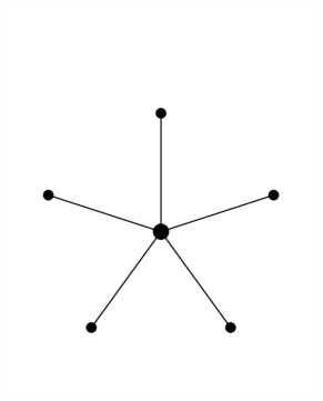
Figure 1: Sketch of a star graph with five bonds of equal length.

We will not allow any dependence of the scattering matrices $\mathcal{S}_{C}$ and $\mathcal{S}_{P}$ on the wave number $k$. Uniqueness of the wave function and the boundary conditions (49) and (52) lead to the quantization condition

$$\boldsymbol{\phi}_{\mathrm{in}}=\mathcal{S}_{P}\mathcal{L}(k)\mathcal{S}_{C}\mathcal{L}(k)\,\boldsymbol{\phi}_{\mathrm{in}}\equiv\mathcal{S}_{B}(k)\,\boldsymbol{\phi}_{\mathrm{in}}$$ (54)

where we introduced the bond scattering matrix $\mathcal{S}_{B}(k)$. Non-trivial solutions of these equations exist only when the wave number belongs to the discrete spectrum $k=k_{n}$ given by the zeros of the corresponding determinant

$$\mathrm{det}\left(\mathcal{S}_{B}(k_{n})-\mathbbm{1}\right)=0.$$ (55)

The density of states for the graph is defined as

$$d(k)=\frac{1}{g}\sum_{n=0}^{\infty}\delta(k-k_{n}),$$ (56)

where $g=2$ in systems with Kramers’ degeneracy (else $g=1$).

IV.2 The trace formula

Let us now write the density of states as a sum of its mean $d_{\mathrm{Weyl}}$ and an oscillating part $\delta d(k)$

$$d(k)=d_{\mathrm{Weyl}}+\delta d(k).$$ (57)

For both contributions one can give an exact semiclassical expression. The mean density of states is given by Weyl’s law

$$d_{\mathrm{Weyl}}=\frac{\mu\sum_{j}L_{j}}{g\pi}$$ (58)

and the oscillating part obeys the trace formula Kottos

$$\delta d(k)=\mathrm{Im}\,\frac{d}{dk}\sum_{n=1}^{\infty}\frac{1}{g\pi\,n}\,\mathrm{tr}\,\mathcal{S}_{B}(k)^{n}.$$ (59)

In the sequel we will consider star graphs where all bond lengths are equal $L_{j}=L$. In that case the bond scattering matrix is a periodic function of $k$

$$\mathcal{S}_{B}(k)=\mathcal{S}_{B}(k+\frac{\pi}{L})=\mathrm{e}^{\mathrm{i}2kL}\tilde{\mathcal{S}}_{B}$$ (60)

where

$$\tilde{\mathcal{S}}_{B}=\mathcal{S}_{B}(k=0)=\mathcal{S}_{P}\mathcal{S}_{C}$$ (61)

is the reduced bond scattering matrix. Thus, the spectrum is also periodic and the trace formula simplifies to

$$d(k)=\frac{\mu B\,L}{g\pi}+\frac{2L}{g\pi}\,\mathrm{Re}\,\sum_{n=1}^{\infty}\mathrm{e}^{\mathrm{i}2nkL}\,\mathrm{tr}\,{\tilde{\mathcal{S}}_{B}}^{n}.$$ (62)

The periodicity of the spectrum will not be relevant here as we are interested in features on the scale of a mean level spacing.

For equal bond lengths the trace formula can be derived in a few lines: Let $\mathrm{e}^{-\mathrm{i}\phi_{j}}$ ($j=1,\dots,\mu B$) be the eigenvalues of the unitary reduced bond scattering matrix $\tilde{\mathcal{S}}_{B}$. The quantization condition (55) is equivalent to $k=\frac{\phi_{j}}{2L}\,\mathrm{mod}\,\frac{\pi}{L}$ ($j=1,\dots,\mu B$) and the density of states is

$$\begin{split}d(k)&=\frac{1}{g}\sum_{j=1}^{\mu B}\sum_{n=-\infty}^{\infty}\delta(k-\frac{\phi_{j}}{2L}+n\frac{\pi}{L})\\ &=\frac{L}{g\pi}\sum_{n=-\infty}^{\infty}\mathrm{e}^{\mathrm{i}2nkL}\sum_{j=1}^{\mu B}\mathrm{e}^{-\mathrm{i}n\phi_{j}}.\end{split}$$ (63)

The mean density of states $d_{\mathrm{Weyl}}=\frac{\mu BL}{g\pi}$ is just the $n=0$ term in the sum over $n$ while the rest gives the trace formula for the oscillating part (the second line follows from the first by Poisson’s summation formula $\sum_{n=-\infty}^{\infty}\delta(x-n)=\sum_{n=-\infty}^{\infty}\mathrm{e}^{\mathrm{i}2\pi nx}$).

The trace formula (59) can be interpreted as a sum over periodic orbits $p$ on the graph. A periodic orbit $p=[(j_{1},\alpha_{1}),(j_{2},\alpha_{2}),\dots(j_{n},\alpha_{n})]$ of length $n$ is defined by a sequence of $n$ peripheral vertices $v_{j_{1}}v_{j_{2}}\dots v_{j_{n}}$ visited one after the other together with the specification of the wave component $\alpha_{j}$ between two vertices (cyclic permutations define the same orbit). A periodic orbit is primitive if it is not the repetition of a shorter periodic orbit. In terms of primitive periodic orbits $p$ and its repetitions the trace formula reads

$$\delta d(k)=\frac{2L}{g\pi}\sum_{\textrm{p.p.o.:}p}\sum_{r=1}^{\infty}n_{p}\left({A_{p}}\mathrm{e}^{\mathrm{i}W_{p}}\right)^{r}$$ (64)

where $n_{p}$ is the length of the primitive periodic orbit $A_{p}=\prod_{l=1}^{n_{p}}{a_{P}}^{(j_{l+1})}_{\alpha_{{l+1}}\alpha_{{l}}}{a_{C}}^{(\alpha_{l})}_{j_{l+1}j_{l}}$ is the amplitude of the primitive orbit and $W_{p}=2n_{p}Lk+\sum_{l=1}^{n_{p}}\left({w_{C}}^{(\alpha_{l})}_{j_{l+1}j_{l}}+{w_{P}}^{(j_{l+1})}_{\alpha_{{l+1}}\alpha_{{l}}}\right)$ its phase (“action”). Note, that we set $j_{n_{p}+1}=j_{1}$ and $\alpha_{n_{p}+1}=\alpha_{1}$.

The similarity of the sum over periodic orbits (64) to the semiclassical Gutzwiller trace formula is evident. However, while semiclassics, in general, is an approximation the semiclassical trace formula for quantum graphs is exact.

The trace formula will be our main tool in the analysis of universal spectral statistics. It will lead us to a simple expression for the form factors that can easily be averaged numerically. In the second paper of this series the trace formula will be in the center of an analytic approach to universality.

Since universality exists on the scale of the mean level spacing we will write $k=\kappa\Delta k$ where $\Delta k=\frac{g\pi}{\mu BL}$ is the mean level spacing. In terms of the rescaled wave number the trace formula is

$$d(\kappa)=1+\frac{2}{\mu B}\,\mathrm{Re}\,\sum_{n=1}^{\infty}\mathrm{e}^{\mathrm{i}2\pi\kappa\frac{gn}{\mu B}}s_{n}.$$ (65)

We have introduced the shorthand

$$s_{n}=\mathrm{tr}\,{\tilde{\mathcal{S}}_{B}}^{n}$$ (66)

for the $n$-th trace of the reduced bond scattering matrix.

The first-order form factor is obtained by a Fourier transform and a subsequent time average. It obeys the trace formula

$$K_{1}(\tau)=\frac{g}{\mu B}\overline{\sum_{n=1}^{\infty}\delta\left(|\tau|-\frac{gn}{\mu B}\right)K_{1,n}}$$ (67)

where the bar denotes a time average over a small time interval $\Delta\tau=\frac{g\Delta n}{\mu B}\ll 1$ and

$$K_{1,n}=\frac{2}{g}\,\left\langle s_{n}\right\rangle.$$ (68)

The brackets $\langle\cdot\rangle$ denote an average over an ensemble of graphs. This can be written more compactly as

$$K_{1}(\tau\equiv\frac{gn}{\mu B})=\overline{K_{1,n}}\equiv\frac{1}{\Delta n}\sum_{k=0}^{\Delta n-1}K_{1,n+k}$$ (69)

where the continuous time average has been replaced by an average over the discrete time $\tau\equiv\frac{gn}{\mu B}$.

The second-order form factor for a graph also obeys a trace formula which, after a spectral average over the central wave number, is given by

$$K_{2}(\tau\equiv\frac{gn}{\mu B})=\overline{K_{2,n}}$$ (70)

where

$$K_{2,n}=\frac{1}{g\mu B}\left\langle\left|s_{n}\right|^{2}\right\rangle.$$ (71)

If no spectral average is performed additional terms appear. These are irrelevant for the graphs in the Wigner-Dyson classes (they do not survive the subsequent ensemble average). Here, we will not consider the second-order form factor for graphs in the novel symmetry classes where the additional terms are relevant near the central energy $\epsilon_{0}=0$.

Though $K_{1,n}$ and $K_{2,n}$ do not involve a time average we will refer to them as (discrete time) form factors.

IV.3 Star graphs for all symmetry classes

We will now construct ensembles of star graphs for each symmetry class. The star graphs will be constructed in such a way that spectral fluctuations of the corresponding ergodic universality classes can be expected. Though we are not able to prove an equivalent conjecture we will give strong evidence.

The constructions of star graphs for each symmetry class are based on a proper choice of the central and peripheral scattering matrices $\mathcal{S}_{C}$ and $\mathcal{S}_{P}$. Both have to obey the right symmetry conditions (see section II).

As an example of star graphs in class $A$I that do not belong to the ergodic universality class let us mention Neumann star graphs. These have a one-component wave function ($\mu=1$) on the bonds, Dirichlet boundary conditions at the peripheral vertices such that $\mathcal{S}_{P}=-\mathbbm{1}$ and Neumann boundary conditions at the center, thus $\mathcal{S}_{C,kl}=\frac{2}{B}-\delta_{kl}$. Such graphs have been investigated first in Kottos and in more detail in gregonstars – in contrast to our approach the bond lengths were chosen different for each bond (and incommensurate). However, Neumann boundary conditions at the center favor backscattering and lead to non-universal (localization) effects gregonstars .

Our approach is different in as much as we allow for more general scattering matrices at the center and in as much as we will always consider an ensemble of graphs. The occurrence or non-occurrence of localization effects can be traced back to a gap condition on the matrix $\mathcal{T}_{ij}\equiv|\mathcal{S}_{C;ij}|^{2}$. This bistochastic matrix describes the corresponding “classical” probabilistic dynamics (equivalent to a Frobenius-Perron operator). In chaotic (ergodic) systems the Frobenius-Perron operator has a finite gap in the spectrum between the (unique) eigenvalue one and all other eigenvalues which describe the decay of the probability distribution. In Neumann star graphs this gap is small and vanishes in the limit $B\rightarrow\infty$ faster than $\frac{1}{B}$ which leads to non-ergodic spectral statistics.

In general one needs a multi-component wave function to introduce the different symmetries. The number of components $\mu$ has been chosen minimal under the additional assumptions that the components do not mix at the central vertex and that time-reversal is only broken at the peripheral vertices.

Though we explicitly choose the central and peripheral scattering matrices guided by simplicity and minimality, most of the results are much more general.

The central scattering can be chosen in a very simple way by using the symmetric $B\times B$ discrete Fourier transform matrix Tanner

$$\mathcal{S}_{\mathrm{DFT},kl}=\frac{1}{\sqrt{B}}\mathrm{e}^{\mathrm{i}2\pi\frac{kl}{B}}$$ (72)

or its complex conjugate for each component. An incoming wave on a given bond is scattered with equal probability to any bond which excludes localization effects. Indeed, the matrix $\mathcal{T}_{\mathrm{DFT},kl}=|\mathcal{S}_{\mathrm{DFT},kl}|^{2}=\frac{1}{B}$ has one eigenvalue $1$ while all other $B-1$ eigenvalues vanish (so the gap is maximal).

The bond scattering matrix $\mathcal{S}_{B}(k)=\mathcal{S}_{C}\mathcal{L}(k)\mathcal{S}_{P}\mathcal{L}(k)$ for each ensemble of graphs is constructed by demanding that the matrices $\mathcal{S}_{C}$, $\mathcal{S}_{P}$, and $\mathcal{L}(k)$ do all have the canonical forms of the desired symmetry class given in section II. Note, that for star graphs we are interested in the $k$ spectrum, so in the canonical forms for scattering matrices the energy $E$ has to be replaced by $k$. The ensemble of graphs is built by introducing some random phases into the peripheral scattering matrix.

IV.3.1 Star graphs in the Wigner-Dyson classes

Let us start with the simplest case: an ensemble of star graphs in class $A$I where a one-component wave-function suffices to incorporate the time-reversal symmetry which demands that the unitary matrices $\mathcal{S}_{C}$, $\mathcal{S}_{P}$, and $\mathcal{L}$ are all symmetric. Now, $\mathcal{S}_{P}$ and $\mathcal{L}(k)=\mathrm{e}^{\mathrm{i}kL}\mathbbm{1}$ are diagonal for $\mu=1$, and choosing

$$\text{$A$I}:\qquad\mathcal{S}_{C}=\mathcal{S}_{\mathrm{DFT}}$$ (73)

we meet all requirements. At the peripheral vertices we are free to choose one random phase $\beta_{k}$ for each peripheral vertex $j$ independently such that

$$\text{$A$I}:\qquad\mathcal{S}_{P,kl}=\delta_{kl}\mathrm{e}^{\mathrm{i}\beta_{k}}$$ (74)

where $0\leq\beta_{k}<2\pi$ is uniformly distributed.

Figure 2: Second-order form factor for star graphs in the Wigner-Dyson ensembles averaged over $10000$ realizations of with $B=100$ bonds (additional time average over an interval of length $8\frac{g}{\mu B}$). Dashed lines: prediction by Gaussian random-matrix theory. Full lines: numerically calculated form factor for graphs. Inlets: discrete time form factor $K_{2,n}$ as function of $\tau=n\frac{g}{\mu B}$ for the class $A$ and $A$I graphs. For the class $A$II graphs $K_{2,n}$ vanishes for odd $n$ – the inlet shows $\frac{K_{2,n}}{2}$ for even $n$.

For class $A$ we have to break time-reversal symmetry. This may be done by choosing a non-symmetric central scattering matrix for a one-component wave-function on the graph. As we like to keep the simplicity of the discrete Fourier transform matrix we choose another simple construction with a two-component wave function, a central $2B\times 2B$ scattering matrix

$$\text{$A$}:\qquad\mathcal{S}_{C}=\begin{pmatrix}\mathcal{S}_{\mathrm{DFT}}&0\\ 0&\mathcal{S}_{\mathrm{DFT}}\end{pmatrix},$$ (75)

and

$$\text{$A$}:\qquad\mathcal{S}_{P}=\frac{1}{\sqrt{2}}\begin{pmatrix}\mathcal{D}_{1}&\mathcal{D}_{2}\\ \mathcal{D}_{3}&\mathcal{D}_{4}\end{pmatrix}$$ (76)

for the peripheral scattering matrix. The diagonal matrices $\mathcal{D}_{j}$ are

$$\text{$A$}:\qquad\begin{array}[]{rl}\mathcal{D}_{1,kl}&=\delta_{kl}\mathrm{e}^{\mathrm{i}(\beta_{k}+\gamma_{k})}\\ \mathcal{D}_{2,kl}&=\delta_{kl}\mathrm{i}\mathrm{e}^{\mathrm{i}(\beta_{k}+\delta_{k})}\\ \mathcal{D}_{3,kl}&=\delta_{kl}\mathrm{i}\mathrm{e}^{\mathrm{i}(\beta_{k}-\delta_{k})}\\ \mathcal{D}_{4,kl}&=\delta_{kl}\mathrm{e}^{\mathrm{i}(\beta_{k}-\gamma_{k})}\end{array}$$ (77)

where the independent random phases $\beta_{k}$, $\gamma_{k}$, and $\delta_{k}$ are uniformly distributed.

For class $A$II a four-component wave-function is needed to incorporate time-reversal invariance with $\mathcal{T}^{2}=-\mathbbm{1}$ into our scheme for star graphs. Indeed, the number of components must be even as discussed above in II.3.1. In addition, we assumed that components do only mix at the peripheral vertices. Then, a $4\times 4$ scattering matrix at the peripheral vertices is the minimal matrix dimension that allows for component mixing as can be seen from the canonical form (16) of a $A$II scattering matrix. The diagonal matrix $\mathcal{L}(k)$ is a diagonal unitary matrix of the canonical form. All further requirements are met by choosing

$$\text{$A$II}:\qquad\mathcal{S}_{C}=\begin{pmatrix}\mathcal{S}_{\mathrm{DFT}}&0&0&0\\ 0&\mathcal{S}_{\mathrm{DFT}}&0&0\\ 0&0&\mathcal{S}_{\mathrm{DFT}}&0\\ 0&0&0&\mathcal{S}_{\mathrm{DFT}}\end{pmatrix}$$ (78)

for the central $4B\times 4B$ scattering matrix, and

$$\text{$A$II}:\qquad\mathcal{S}_{P}=\frac{1}{\sqrt{2}}\begin{pmatrix}0&\mathcal{D}_{1}&0&\mathcal{D}_{2}\\ \mathcal{D}_{3}&0&-\mathcal{D}_{2}&0\\ 0&-\mathcal{D}_{4}&0&\mathcal{D}_{3}\\ \mathcal{D}_{4}&0&\mathcal{D}_{1}&0\end{pmatrix}$$ (79)

for the peripheral scattering matrix. The diagonal matrices $\mathcal{D}_{j}$ are given by

$$\text{$A$II}:\qquad\begin{array}[]{rl}\mathcal{D}_{1,kl}&=\delta_{kl}\mathrm{e}^{\mathrm{i}(\beta_{k}+\gamma_{k})}\\ \mathcal{D}_{2,kl}&=\delta_{kl}\mathrm{e}^{\mathrm{i}(\beta_{k}+\delta_{k})}\\ \mathcal{D}_{3,kl}&=\delta_{kl}\mathrm{e}^{\mathrm{i}(\beta_{k}-\gamma_{k})}\\ \mathcal{D}_{4,kl}&=\delta_{kl}\mathrm{e}^{\mathrm{i}(\beta_{k}-\delta_{k})},\end{array}$$ (80)

where the independent random phases $\beta_{k}$, $\gamma_{k}$, and $\delta_{k}$ are uniformly distributed.

Ergodic spectral statistics may be expected for the three ensembles in The Wigner-Dyson classes. This is strongly supported by a numerical calculation of the second-order form factor (see figure 2).

IV.3.2 Chiral and Andreev star graphs

Figure 3: First-order form factor for Andreev star graphs in the classes $C$ and $C$I averaged over $10000$ realizations with $B=100$ bonds (additional time average over an interval of length $8\frac{g}{\mu B}$). Dashed lines: prediction by Gaussian random-matrix theory. Full lines: numerically calculated form factor for graphs. Inlets: discrete time form factor $\frac{K_{1,n}}{2}$ as function of $\tau=n\frac{g}{\mu B}$ for even $n$ ($K_{1,n}$ vanishes by construction for odd $n$).

Let us start with the Andreev star graphs for the classes $C$ and $C$I where the wave function can be chosen in the simplest case to have two components. The first will be called “electron” and the second “hole”. The transfer matrix $\mathcal{L}(k)$ and the central scattering matrix defined by

$$\left.\begin{array}[]{l}\text{$C$}\\ \text{$C$I}\end{array}\right\}:\qquad\mathcal{S}_{C}=\begin{pmatrix}\mathcal{S}_{\mathrm{DFT}}&0\\ 0&\mathcal{S}_{\mathrm{DFT}}^{*}\end{pmatrix}$$ (81)

obey the symmetry condition (27).

Figure 4: The first-order form factor for Andreev star graphs in the classes $D$ and $D$III (see figure 3 for details).

The peripheral scattering matrix may be chosen such that complete Andreev scattering (electron-hole conversion) takes place

$$\left.\begin{array}[]{l}\text{$C$}\\ \text{$C$I}\end{array}\right\}:\qquad\mathcal{S}_{P}=\frac{1}{\sqrt{2}}\begin{pmatrix}0&\mathcal{D}\\ -\mathcal{D}^{*}&0\end{pmatrix}$$ (82)

where the diagonal matrix $\mathcal{D}$ is

$$\text{$C$}:\qquad\mathcal{D}_{kl}=\delta_{kl}\,\mathrm{e}^{\mathrm{i}\beta_{k}}$$ (83)

for class $C$, and

$$\text{$C$I}:\qquad\mathcal{D}_{kl}=\delta_{kl}\,\mathrm{i}\sigma_{k}$$ (84)

for class $C$I. The random phases $\beta_{k}$ are uniformly distributed and $\sigma_{k}=\pm 1$ with equal probability.

For the Andreev classes $D$ and $D$III and as well for the three chiral classes $A$III, $BD$I, and $C$II a four-component wave function is needed. We will call the first (last) two components “electron” (“hole”).

​

​

Figure 5: The first-order form factor for chiral star graphs (see figure 3 for details).

The symmetry requirements (28), (29), (20), (21), and (22) are met by the transfer matrix $\mathcal{L}(k)$ and the central scattering matrix defined by

$$\left.\begin{array}[]{l}\scriptstyle\text{$D$}\\ \scriptstyle\text{$D$III}\\ \scriptstyle\text{$A$III}\\ \scriptstyle\text{$BD$I}\\ \scriptstyle\text{$C$II}\end{array}\right\}:\;\;\mathcal{S}_{C}=\begin{pmatrix}\mathcal{S}_{\mathrm{DFT}}&0&0&0\\ 0&\mathcal{S}_{\mathrm{DFT}}&0&0\\ 0&0&\mathcal{S}_{\mathrm{DFT}}^{*}&0\\ 0&0&0&\mathcal{S}_{\mathrm{DFT}}^{*}\end{pmatrix}.$$ (85)

In all five remaining classes we choose the peripheral scattering matrix such that complete Andreev scattering takes place. For $D$ and $D$III the simplest choice obeying the symmetry requirements are

$$\left.\begin{array}[]{l}\text{$D$}\\ \text{$D$III}\end{array}\right\}:\;\;\mathcal{S}_{P}=\frac{1}{\sqrt{2}}\begin{pmatrix}0&0&\mathcal{D}_{1}&\mathcal{D}_{2}\\ 0&0&-\mathcal{D}_{2}^{*}&\mathcal{D}_{1}^{*}\\ \mathcal{D}_{1}^{*}&\mathcal{D}_{2}^{*}&0&0\\ -\mathcal{D}_{2}&\mathcal{D}_{1}&0&0\\ \end{pmatrix}$$ (86)

where the diagonal matrices $\mathcal{D}_{j}$ are

$$\text{$D$}:\qquad\begin{array}[]{rl}\mathcal{D}_{1,kl}&=\delta_{kl}\,\mathrm{e}^{\mathrm{i}\beta_{k}}\\ \mathcal{D}_{2,kl}&=\delta_{kl}\,\mathrm{e}^{\mathrm{i}\gamma_{k}}\end{array}$$ (87)

for class $D$, and

$$\text{$D$III}:\qquad\begin{array}[]{rl}\mathcal{D}_{1,kl}&=\delta_{kl}\,\mathrm{e}^{\mathrm{i}\beta_{k}}\\ \mathcal{D}_{2,kl}&=\delta_{kl}\,\mathrm{i}\sigma_{k}\end{array}$$ (88)

for class $D$III. The random phases $\beta_{k}$ and $\gamma_{k}$ are uniformly distributed and $\sigma_{k}=\pm 1$ with equal probability.

The simplest choice for peripheral scattering matrices in the chiral classes is

$$\left.\begin{array}[]{l}\text{$A$III}\\ \text{$BD$I}\\ \text{$C$II}\end{array}\right\}:\;\mathcal{S}_{P}=\frac{1}{\sqrt{2}}\begin{pmatrix}0&0&\mathcal{D}_{1}&\mathcal{D}_{2}\\ 0&0&\mathcal{D}_{3}&-\mathcal{D}_{1}\\ \mathcal{D}_{4}&\mathcal{D}_{5}&0&0\\ \mathcal{D}_{6}&-\mathcal{D}_{4}&0&0\end{pmatrix}.$$ (89)

The diagonal matrices $\mathcal{D}_{j}$ have to be chosen according to the requirements of each symmetry class. For class $A$III they are

$$\text{$A$III}:\qquad\begin{array}[]{rl}\mathcal{D}_{1,kl}&=\delta_{kl}\sigma_{k}\\ \mathcal{D}_{2,kl}&=\delta_{kl}\mathrm{e}^{\mathrm{i}\beta_{k}}\\ \mathcal{D}_{3,kl}&=\delta_{kl}\mathrm{e}^{-\mathrm{i}\beta_{k}}\\ \mathcal{D}_{4,kl}&=\delta_{kl}\tau_{k}\\ \mathcal{D}_{5,kl}&=\delta_{kl}\mathrm{e}^{\mathrm{i}\gamma_{k}}\\ \mathcal{D}_{6,kl}&=\delta_{kl}\mathrm{e}^{-\mathrm{i}\gamma_{k}}\end{array}$$ (90)

where $\tau_{k},\sigma_{k}=\pm 1$ with equal probability and the phases $\beta_{k}$ and $\gamma_{k}$ are uniformly distributed. The $BD$I star graphs can be obtained from the $A$III case by the additional restrictions

$$\text{$BD$I}:\qquad\tau_{k}=\sigma_{k}\qquad\text{and}\qquad\gamma_{k}=-\beta_{k}.$$ (91)

Finally, for class $C$II the peripheral scattering matrix is defined by

$$\text{$C$II}:\qquad\begin{array}[]{rl}\mathcal{D}_{1,kl}&=\delta_{kl}\sigma_{k}\\ \mathcal{D}_{2,kl}&=\delta_{kl}\mathrm{e}^{\mathrm{i}\beta_{k}}\\ \mathcal{D}_{3,kl}&=\delta_{kl}\mathrm{e}^{-\mathrm{i}\beta_{k}}\\ \mathcal{D}_{4,kl}&=-\delta_{kl}\sigma_{k}\\ \mathcal{D}_{5,kl}&=-\delta_{kl}\mathrm{e}^{\mathrm{i}\beta_{k}}\\ \mathcal{D}_{6,kl}&=-\delta_{kl}\mathrm{e}^{-\mathrm{i}\beta_{k}}\end{array}$$ (92)

We have checked numerically that the first-order form factor for the constructed Andreev and chiral star graphs obeys the corresponding prediction by Gaussian random-matrix theory (see figures 3,4, and 5).

- (1) E.P. Wigner, Ann. Math. 67, 325 (1958).
- (2) F.J. Dyson, J. Math. Phys. 3, 140, 1199 (1962).
- (3) C.E. Porter (ed.), Statistical Theories of Spectra, (Academic, New York 1965).
- (4) M.L. Mehta, Random Matrix Theory and the Statistical Theory of Spectra, (Academic, New York 1967, 2nd edition 1991).
- (5) T. Guhr, A. Müller-Groeling, and H.A. Weidenmüller, Phys. Rep. 299, 189 (1998).
- (6) O. Bohigas, M.J. Giannoni, and C. Schmit, Phys. Rev. Lett. 52, 1 (1984).
- (7) J.J.M. Verbaarschot and I. Zahed, Phys. Rev. Lett. 70, 3852 (1993); J.J.M. Verbaarschot, ibid 72, 2531 (1994).
- (8) A. Altland and M.R. Zirnbauer, Phys. Rev. B 55, 1142 (1997).
- (9) M.R. Zirnbauer, J. Math. Phys. 37, 4989 (1996).
- (10) T. Kottos and U. Smilansky, Phys. Rev. Lett 79, 4794 (1997); Ann. Phys. 274, 76 (1999).
- (11) S. Gnutzmann, and B. Seif, to be published.
- (12) S. Gnutzmann, B. Seif, F. von Oppen, and M. Zirnbauer, Phys. Rev. E 67, 046225 (2003).
- (13) B. Seif, dissertation thesis (Köln 2003).
- (14) Ph. Jacquod, H. Schomerus, and C.W.J. Beenakker Phys. Rev. Lett. 90, 207004 (2003).
- (15) Y.V. Fyodorov and A.D. Mirlin, Phys. Rev. Lett. 67, 2405 (1991).
- (16) J.A. Melsen, P.W. Brouwer, K.M. Frahm, and C.W.J. Beenakker, Europhys. Lett. 35, 7 (1996).
- (17) M.C. Gutzwiller, J. Math. Phys. 12, 343 (1971)
- (18) T. Nagao and K. Slevin, J. Math. Phys. 34, 2317 (1993).
- (19) T. Wettig, habilitation thesis (Heidelberg 1998).
- (20) D.A. Ivanov, J. Math. Phys. 43, 126 (2002).
- (21) M. Abramowitz,and I.A. Stegun, Handbook of Mathematical Functions (Dover, New York, 1965).
- (22) J.P. Keating, Nonlinearity 4, 277 (1991); Nonlinearity 4, 309 (1991).
- (23) E.B. Bogomolny, B. Georgeot, M.J. Giannoni, and C. Schmit, Phys. Rep. 291, 219 (1997).
- (24) N. Argaman, Y. Imry, and U. Smilansky, Phys. Rev. B 47 4440.
- (25) N. Argaman, F. Dittes, E. Doron, J. Keating, A. Kitaev, M. Sieber and U. Smilansky, Phys. Rev. Lett. 71, 4326 (1993).
- (26) O. Agam, B.L. Altshuler, A.V. Andreev, Phys. Rev. Lett. 75, 4389 (1995).
- (27) M. Sieber, and K. Richter, Phys. Scr. T 90, 128 (2001); M. Sieber, J. Phys. A 35, L613-L619 (2002).
- (28) G. Berkolaiko, and J.P. Keating, J. Phys. A 32,7827 (1999); G. Berkolaiko, E.B. Bogomolny, and J.P. Keating,J. Phys. A 34, 335 (2001).
- (29) G. Tanner, J. Phys. A 34, 8485 (2001).