Trapping in quantum chains

Abstract

A quantum breather on a translationally invariant one-dimensional anharmonic lattice is an extended Bloch state with two or more particles in a strongly correlated state. We discuss several effects that break the lattice symmetry and lead to spatial localization of the breather.

PACS: 63.20.Pw

Keywords: Anharmonic quantum lattices, Quantum breathers, Quantum lattice solitons

1 Introduction

The localization of energy by nonlinearity in classical lattices has been much studied in the last 20 years. The corresponding localized states, known as intrinsic localized modes or discrete breathers, have been the subject of intense theoretical and experimental investigation [1]. Corresponding results on the quantum equivalent of discrete classical breathers are less numerous, c.f. [2, 3] for some theoretical results and [4] for some experimental work. Studies of quantum modes on small lattices may be relevant to studies of quantum dots and quantum computing (c.f. [5]).

In this paper, we present some results related to quantum lattice problems, in particular in one dimensional lattices with a small number of quanta. We study a periodic lattice with $f$ sites containing bosons, described by the quantum discrete nonlinear Schrödinger equation (QDNLS), a quantum version of the discrete nonlinear Schrödinger equation (also know as the Boson Hubbard model). The DNLS equation describes a particularly simple model for a lattice of coupled anharmonic oscillators, and it has been used to describe the dynamics of a great variety of systems [6]. The corresponding quantum Hamiltonian is given by

$$\hat{H}=-\sum_{j=1}^{f}\frac{1}{2}\gamma_{j}b_{j}^{\dagger}b_{j}^{\dagger}b_{j}b_{j}+\epsilon_{j}b_{j}^{\dagger}(b_{j-1}+b_{j+1}),$$ (1)

where $b_{j}^{\dagger}$ and $b_{j}$ are standard bosonic operators, $\gamma_{j}/\epsilon_{j}$ is the ratio of anharmonicity to nearest neighbor hopping energy, and the chain is subject to periodic boundary conditions with period $f$. Initially we consider the case where the chain is translationally invariant, i.e. $\gamma_{j}=\gamma$ and $\epsilon_{j}=\epsilon$ are independent of $j$. In general we take $\epsilon=1$.

The Hamiltonian (1) has an important conserved quantity, the number $N=\sum_{j=1}^{f}b_{j}^{\dagger}b_{j}$, which enables the total Hamiltonian to be block-diagonalised and greatly simplifies the analysis. In this letter we restrict ourselves to the simplest nontrivial case $N=2$, though many of the results are valid for larger values on $N$. The $N=2$ bound states corresponds to bound two-vibron states, as observed experimentally in several systems [7].

In QDNLS case, we use a number state basis, $|\psi_{n}\rangle=[n_{1},n_{2},...,n_{f}]$, where $n_{i}$ represents the number of quanta at site $i$ ($N=\sum n_{i}$). A general wave function is $|\Psi_{n}\rangle=\sum_{n}c_{n}|\psi_{n}\rangle$.

In homogeneous quantum lattices with periodic boundary conditions, it is possible to block–diagonalize the Hamiltonian operator using eigenfunctions of the translation operator with fixed value of the momentum $k$ [2].

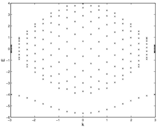
Figure 1: Eigenvalues $E(k)$ for QDNLS model with periodic boundary conditions. $N=2$, $f=19$, $\gamma=4$.

As shown in Fig. 1, if the anharmonicity parameter is high enough, there exists an isolated eigenvalue for each $k$ which corresponds to a localized eigenfunction. By this we mean there is a high probability of finding the two quanta on the same site, but due to the translational invariance of the system, an equal probability of finding these two quanta at any site of the system. In these cases, some analytical expressions can be obtained in some asymptotic limits (solutions of this problem go back to the 30’s, for recent discussions see [6, 2, 8]).

In particular, working at $k=0$ for simplicity, the ground state unnormalized eigenfunction is

$$|\Psi\rangle=[20\dots 0]+[020\dots 0]+\dots+[0\dots 02]+O(\gamma^{-1}),$$

i.e. on a lattice of length $f$, the unnormalized coefficients $c_{i}$ of the first $f$ terms are equal to unity and the rest are $O(\gamma^{-1})$. In the other extreme of complete spatial localization, one of these $c_{i}$ would be unity and the rest zero. In this letter we consider how these components change as the translational invariance of the lattice is broken in various ways.

One simple way that translational invariance can be broken is by considering a finite chain with no-flux boundary conditions. The Hamiltonian operator now cannot be block-diagonalized using eigenvectors of the translation operator. In this case, the computational effort increases, but it is still possible to calculate the all the eigenvalues and eigenvectors of the Hamiltonian operator, if $f$ and $N$ are small enough, by using algebraic manipulation methods and numerical eigenvalue solvers.

The existence of local inhomogeneities or impurities in a system can affect the nonlinear localized modes considerably. Also, in systems with both nonlinearity and impurities, it is important to understand the interplay between these two sources of localization. For these cases we break translational invariance by making one or more of the $\gamma_{j}$ or the $\epsilon_{j}$ depend on $j$. This may occur because of localized impurities, or because the chain geometry becomes non-uniform. Two examples of non-uniform geometries are shown in Fig. 2.

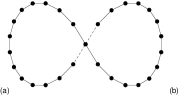
Figure 2: Two non-uniform chain geometries

Fig. 2a shows a circular chain twisted into a figure-of-eight, so that two sites on the chain, which are distant measured along the length of the chain, become spatially close. This toy model for a globular protein was studied in [9], where it was shown that moving breathers described by the classical DNLS equation could become trapped at the cross-over point. In the quantum case such a geometry can be modeled by adding a term such as

$$\alpha_{\ell,m}(b_{\ell}^{\dagger}b_{m}+b_{m}^{\dagger}b_{\ell}),$$ (2)

to the Hamiltonian, where $\ell$ and $m$ are the two sites brought close together by the twist, and $\alpha_{\ell,m}$ is the separation distance relative to the unit length of the unperturbed chain. This can be considered as a special case of a chain with long-range coupling. See also [10] for a more realistic protein simulation, and [11] for other discussions on the effects of chain geometry on moving breathers.

The bent chain in Fig. 2b shows another possible geometry which has been studied recently in the classical DNLS case. In this case we have an abrupt bend which is simulated by adding an additional term as in (2) but where $m=m_{0}-1,\ell=m_{0}+1$, where $m_{0}$ is the vertex of the bend. By varying the values of $\alpha_{\ell,m}=\alpha$, all angles between 0 and $\pi$ can be simulated approximately. The influence of this geometry has been analyzed in the DNLS context in [12], and in nonlinear Klein–Gordon systems in [13]. This geometry is of interest in nonlinear photonic crystals waveguides and circuits [14].

Localization due to random variation of the lattice parameters has long been studied in the harmonic model since the pioneering work of Anderson [15]. Our interest is to see what new localization effects the anharmonic terms bring to the model, and to what extent the anharmonic effects enhance the Anderson-like localization effect when this is present in the harmonic model ($\gamma_{i}=0$). See also the discussions in [16].

Most of our findings are not specific to the QDNLS model, for example we have repeated our calculations using the attractive fermionic Hubbard model with two particles of opposite spins. Details will be given elsewhere. Although all the models we consider have a conserved number, in general they are not quantum integrable.

We now consider the effects introduced above in more detail.

2 Localization in an straight chain with impurities

In this version of our model, in order to explore the interplay between the localization induced by the nonlinearity and the influence of a impurity in these localized states, we introduce a local inhomogeneity in the anharmonic parameter. To isolate the effect of the impurity of other effects related to the finite size of the chain, we retain the periodic boundary conditions. The anharmonicity parameter is $\gamma_{\ell}=\gamma_{\text{im}}$, and $\gamma_{j}=\gamma$ for $j\neq\ell$.

In the homogeneous system ($\gamma_{\text{im}}=\gamma$), with $\gamma$ large enough, as discussed above, the ground state is a localized in the sense that there exist a high probability to find the two quanta on the same site, but with equal probability at any site of the chain. For the chain with a point impurity, we plot in Fig. 3 the coefficients of some of the components of the ground state wave function for various values of $\gamma_{\text{im}}$.

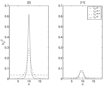
Figure 3: QDNLS model with point impurity, $\gamma=4$, $N=2$, $f=19$.

The left hand figure shows the coefficients of the $[20\dots],[020\dots],\dots$ components. As $\gamma_{\text{im}}$ increases, these coefficients start from an initial spatially uniform distribution, but then localize around the site of the impurity, in this case at $\ell=10$. At the largest value of $\gamma_{\text{im}}$ shown, over 60% of the wave function is in the state $[0\dots 020\dots]$, with the two bosons at site 10.

The right hand figure shows the corresponding coefficients of the $[110\dots],[0110\dots],\dots$ components. Again some localization is found as $\gamma_{\text{im}}$ increases, but this effect is much weaker for these components. Other components are even smaller.

In Fig. 4, we plot the size of the first three components of the type $[2],[11],[101]$ respectively, centred around site 10, as a function of $\gamma_{\text{im}}-\gamma$. The localization increases very rapidly with the magnitude of the impurity.

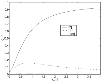
Figure 4: Some components of the wave function corresponding to the ground state, $N=2,f=19$, $\gamma=4$.

Note that there is no Anderson-like effect in this case as the harmonic terms are homogeneous.

3 The twisted chain

For the twisted chain as shown in Fig. 2a, the only extra parameter is $\alpha_{m,\ell}$, the strength of the long range coupling between the two spatially adjacent sites $m$ and $\ell$. As an example we consider the case $\alpha_{m,\ell}=1,f=19,m=5$, and $\ell=15$. Fig. 5 shows two sets of components of the ground state wave function, plotted as a function of $\gamma$.

Figure 5: QDNLS model with twisted chain, $\gamma=4.0$, $N=2$, $f=19$

The components here are the same as those plotted in Fig. 3, with a crossover point at $m=5,\ell=15$. A breather localized at the crossover point will show an enhanced coefficient corresponding to localization at the two points of the chain which come together. With $\gamma=0$, we see some small localization effect at sites $m$ and $\ell$ for the $[2]$ coefficients at the crossover points, corresponding to a harmonic Anderson-like effect. However for nonzero $\gamma$ we see that this effect is strongly enhanced. The coefficient of the $[11]$ component show a weaker localization as before. Similar results are obtained for other values of $\alpha_{m,\ell}$, with the strength of the localization depending on the size of $\alpha_{m,\ell}$. These trapped quantum states simulate the trapping of the classical mobile breather studied in [9].

4 The Bent Chain

For the bent QDNLS chain Fig. 2, we follow the classical DNLS treatment [12]. We consider the Hamiltonian (1) on a finite lattice with the additional term (2). The parameter $\alpha$ is related to the wedge angle $\theta$ through $\alpha=\frac{1}{2}(1-\cos\theta)^{-1}$, and we take the site of the vertex to be $m_{0}=\frac{1}{2}(f+1)$.

Fig. 6 shows the coefficients of the $[2],[11],[101]$ components of the wave function for various values of $\theta$.

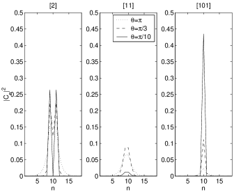
Figure 6: QDNLS bent chain model, $N=2$, $f=19$, $\gamma=4$.

Fig. 7 shows some components of the ground state wave function corresponding to the neighbors of the vertex, for both $\gamma=0$ and $\gamma=4$. If the angle $\theta$ is close to $\pi$, the behavior is similar to the straight chain. The ground state is weakly localized around the center (vertex) of the chain. As $\theta$ decreases, the localization around the vertex increases, and when this angle is small enough, the largest components of the wave function in the ground state consists of states localized around the vertex and the two connected neighboring sites. In the limit $\theta\rightarrow 0$, the lattice becomes a T-junction, a model of interest in its own right. It is interesting that the localization in the anharmonic model exhibits a maximum at $\theta\approx 0.5$, whereas in the harmonic case the maximum is at $\theta=0$. Also the enhancement due to the anharmonic terms goes to zero as $\theta\rightarrow 0$.

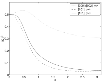
Figure 7: QNLS bent chain, $N=2,f=19$, various $\gamma$.

In this paper, we have considered only a long–range interaction between the two vertices of the chain. We have also studied more realistic models with long–range interaction between all neighbors in the chain. Qualitatively the same localization phenomena is observed: a full description will be given elsewhere.

References

- [1] S. Flach and C.R. Willis, Phys. Rep. 295, 181 (1998); Physica D 119, special volume edited by S. Flach and R.S. Mackay (1999): P.G. Kevrekidis, K.Ø. Rasmussen and A.R. Bishop, Int. J. Mod. Phys. B, 15, 2833 (2001); focus issued edited by Yu. S. Kivshar and S. Flach, Chaos 13, 586 (2003), Localization and Energy Transfer in Nonlinear Systems, eds L. Vázquez, R. S. MacKay, M. P. Zorzano (World Scientific, Singapore, 2003).
- [2] A.C. Scott, J.C. Eilbeck and H. Gilhøj, Physica D 78, 194 (1994).
- [3] V. Fleurov, Chaos 13, 676 (2003); R.S. MacKay, Physica A 288, 174 (2000).
- [4] F. Fillaux, C.J. Carlile and G.J. Kearley, Phys. Rev. B 58, 11416 (1998); B.I. Swanson et al. Phys. Rev. Lett. 82, 3288 (1999); T. Asano et al., Phys. Rev. Lett. 84, 5880 (2000); L.S. Schulman et. al., Phys. Rev. Lett. 88, 224101, (2002).
- [5] Xiaoqin Li et al., Science 301, 809 (2003).
- [6] A.C. Scott, Nonlinear Science (OUP, Oxford 1999).
- [7] P. Jakob, Appl. Phys. A: Mater. Sci. Proc. 75, 45 (2002).
- [8] J.C. Eilbeck, in Localization and Energy Transfer in Nonlinear Systems, World Scientific, Singapore, 177 (2003).
- [9] J.C. Eilbeck, in Computer Analysis for Life Science, eds. C. Kawabata and A.R Bishop, 12 (Ohmsha: Tokyo 1986).
- [10] H. Feddersen, Phys Lett A 154, 391 (1991).
- [11] P.G. Kevrekidis, B.A. Malomed and A.R. Bishop, Phys. Rev. E 66, 046621 (2002); I. Baena, A. Saxena and J.M. Sancho, Phys. Rev. E 65, 036611 (2002); J. Cuevas, F. Palmero, J.F.R. Archilla and F.R. Romero, Phys. Lett. A 299, 221 (2002).
- [12] P.L. Christiansen, Y.B. Gaididei and S.F. Mingaleev, J. Phys. Condens. Matter 13, 1181 (2001); Yu.S. Kivshar, P.G. Kevrekidis and S. Takeno, Phys. Lett. A 307, 287 (2003).
- [13] J. Cuevas and P.G. Kevrekidis, Preprint (2003).
- [14] S.F. Mingaleev and Yu.S. Kivshar, Opt. Photonics News 13, 48 (2002).
- [15] P.W Anderson, Phys. Rev. 109, 1492 (1958).
- [16] J.F.R Archilla, R.S. MacKay, and J.L. Marin, Physica D 134, 406 (1999); G. Kopidakis and S. Aubry, Physica D 139, 247 (1999).