Shear dispersion along circular pipes is affected by bends, but the torsion of the pipe is negligible

Abstract

The flow of a viscous fluid along a curving pipe of fixed radius is driven by a pressure gradient. For a generally curving pipe it is the fluid flux which is constant along the pipe and so I correct fluid flow solutions of Dean (1928) and Topakoglu (1967) which assume constant pressure gradient. When the pipe is straight, the fluid adopts the parabolic velocity profile of Poiseuille flow; the spread of any contaminant along the pipe is then described by the shear dispersion model of Taylor (1954) and its refinements by Mercer, Watt et al. (1994,1996). However, two conflicting effects occur in a generally curving pipe: viscosity skews the velocity profile which enhances the shear dispersion; whereas in faster flow centrifugal effects establish secondary flows that reduce the shear dispersion. The two opposing effects cancel at a Reynolds number of about $15$. Interestingly, the torsion of the pipe seems to have very little effect upon the flow or the dispersion, the curvature is by far the dominant influence. Lastly, curvature and torsion in the fluid flow significantly enhance the upstream tails of concentration profiles in qualitative agreement with observations of dispersion in river flow.

1 Introduction

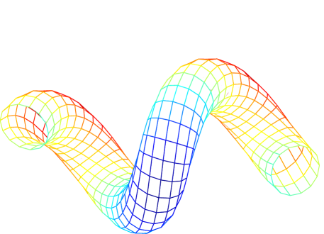
Figure 1: perspective figure of a helical pipe as an example of the curving pipes containing fluid flow and contaminant dispersion that is modelled herein. On the right is a schematic diagram of the orthogonal curvilinear coordinate system local to the curving centre line of the pipe: $u$ points along the centre line and $s$ measures axial distance.

Consider the dispersion of a contaminant, with diffusivity $\kappa_{c}$, in the steady laminar flow, velocity field $q$, of a Newtonian fluid of density $\rho$ and kinematic viscosity $\nu$ in an arbitrarily curving pipe of radius $a$ such as the helical pipe shown in Figure 1. The flow is pumped by an overall pressure drop which maintains a fixed fluid flux along the pipe; that is, a constant mean velocity $U$ is maintained irrespective of curvature. Non-dimensionalise quantities with respect to the pipe radius $a$, the cross-pipe diffusion time $a^{2}/\kappa_{c}$, and the reference pressure $\rho\nu U/a$. The Navier-Stokes and continuity equations for the steady, incompressible fluid flow then become

$${\cal R}\mbox{\boldmath$q$}\cdot\mbox{\boldmath$\nabla$}\mbox{\boldmath$q$}=-\mbox{\boldmath$\nabla$}p+\nabla^{2}\mbox{\boldmath$q$}\quad\mbox{and}\quad\mbox{\boldmath$\nabla$}\cdot\mbox{\boldmath$q$}=0\,,$$ (1)

where ${\cal R}=aU/\nu$ is the Reynolds number. The contaminant evolves according to the non-dimensional advection-diffusion equation

$$\frac{\partial c}{\partial t}+{\cal P}\mbox{\boldmath$q$}\cdot\mbox{\boldmath$\nabla$}c=\nabla^{2}c\,,$$ (2)

where ${\cal P}=aU/\kappa_{c}$ is the Peclet number. In typical liquids the Peclet number is much larger than the Reynolds number as their ratio, the Schmidt (or Prandtl) number $\sigma={\cal P}/{\cal R}=\nu/\kappa_{c}$, is normally large: approximately $10^{3}$ for the diffusion of material in liquids [28, p1119, e.g.]; although only about $8$ for the diffusion of heat [1, p597]; whereas in typical gases the Schmidt number is roughly $1$ and so the Peclet and Reynolds numbers are comparable. The analysis is interpreted with these two cases in mind of the Schmidt number being either ${\cal O}\big{(}1000\big{)}$ or ${\cal O}\big{(}1\big{)}$.

Here we analyse the flow and dispersion in an arbitrarily curving circular pipe. Most analysis of dispersion assumes a curved pipe is toroidal [28, 23, 14, 6, e.g.] and most experiments are performed in helical pipes [33, e.g.] (see further discussion by Berger et al. [3]). Neglecting molecular diffusivity, dispersion in toroidal flow has been characterised from analytic formulae by Ruthven [28] and numerical solutions by McConalogue [20] using the residence time of different streamlines. Interestingly, using similar ideas Jones [15] deduced a regime of anomalous dispersion in a twisted but piecewise toroidal pipe. The fluid flow in helical pipes has been the subject of recent analysis [12, 34, 19, 38, e.g.], whereas the flow in arbitrarily curving and twisting pipes has received little attention although Pedley [24] accounted for leading order effects of variable curvature but ignored torsion, and Gammack & Hydon [11] investigate flow in pipes with exponentially varying curvature and torsion. Here I take these analyses further by simultaneously determining the fluid flow and the dispersion in arbitrarily curving circular pipes. The analysis is restricted to parameter regimes where the fluid flow is laminar—because of the induced secondary circulation, laminar flow is stable to higher Reynolds numbers in a curving pipe [33, 3]. The results thus will also be important in the flow and dispersion in microfluidic channels [13, e.g.].

In §2.1 we establish an orthogonal coordinate system based upon the arbitrarily curving geometry of the circular pipe, although requiring that the curvature of the centre line varies smoothly. Let the centre line of the pipe be described by $\mbox{\boldmath$R$}(s)$ where $s$ measures arclength along the centre line. Then a useful set of vectors for space in the vicinity of the pipe are the unit tangent $\mbox{\boldmath$u$}(s)=\mbox{\boldmath$R$}^{\prime}$ of the centre curve, unit normal $\mbox{\boldmath$p$}(s)$ and the unit binormal $\mbox{\boldmath$b$}(s)$ (see Figure 1). These vectors and the curvature $\kappa(s)$ and torsion $\tau(s)$ of the pipe are all connected by the Frenet formulae [17, §8.7,e.g.]

$$\mbox{\boldmath$u$}^{\prime}=\kappa\mbox{\boldmath$p$}\,,\quad\mbox{\boldmath$p$}^{\prime}=-\kappa\mbox{\boldmath$u$}+\tau\mbox{\boldmath$b$}\,,\quad\mbox{\boldmath$b$}^{\prime}=-\tau\mbox{\boldmath$p$}\,.$$ (3)

Throughout this article I use a dash to denote $\partial/\partial s$. In a thin pipe the non-dimensional velocity is approximately Poiseuille flow, $u\approx 2(1-r^{2})$. However, there are corrections of ${\cal O}\big{(}\kappa\big{)}$ due to the curvature which are determined by solving the Navier-Stokes equations (1) for the fluid flow, see §2 where low order expressions agree with the careful analysis of the flow in helical pipes by Tuttle [34].

Centre manifold theory provides a rationale to form low-dimensional models of dynamics as I elaborated in the overview [27]. Here we model the long-time evolution of the large scale dispersion of contaminant along the pipe. Models of “long-waves” or “slowly varying in space” dynamics are justified in the centre manifold approach by requiring resolved longitudinal spatial structures to have small wavenumber [25]. With this proviso, diffusion acts relatively quickly across the pipe to cause the contaminant concentration to be approximately constant in any cross-section: to leading order $c\approx C(s,t)$ where $C=\bar{c}$ is an average over a pipe cross-section. The centre manifold analysis then systematically accounts for how variations along the pipe are affected by the varying velocity profile to disperse the contaminant. We thus deduce in §3, as a generalisation of Taylor’s model [30, 31], the advection-diffusion model

$$\frac{\partial C}{\partial t}\approx-{\cal P}\frac{\partial C}{\partial s}+\frac{\partial\ }{\partial s}\left(D\frac{\partial C}{\partial s}\right)\,,$$ (4)

where for the case of a pipe of circular cross-section the effective diffusivity

$$D \!\!\!=\!\!\! \left(1+\frac{\kappa^{2}}{4}\right)+\frac{{\cal P}^{2}}{48}\left[1+\kappa^{2}\left(\frac{863}{120}-\frac{7267{\cal R}^{2}}{241920}+\frac{599{\cal R}^{4}}{48384000}-\frac{2569\sigma^{2}{\cal R}^{4}}{68428800}\right)\right]$$ (5)

$${}+{\cal O}\big{(}\kappa^{4},\delta\big{)}\,.$$

That is, the shear dispersion in a straight pipe, $D={\cal P}^{2}/48$, is in a curved pipe modified by a factor approximately

$$1+\kappa^{2}\left[7.2-3.0\left(\frac{{\cal R}}{10}\right)^{2}+(0.12-0.38\sigma^{2})\left(\frac{{\cal R}}{10}\right)^{4}\right]\,,$$

As found by others, secondary circulation caused by fluid inertia depresses the effective dispersion, by about $\kappa^{2}[3.0({\cal R}/10)^{2}+0.38\sigma^{2}({\cal R}/10)^{4}]$ , but only for Reynolds numbers sufficiently large. In slow viscous flow, pipe curvature actually enhances the effective dispersion by about $7.2\kappa^{2}$—an effect that has apparently often been neglected [33, p317] in experimental determination of dispersion coefficients.

• For dispersion in gas flow, with ${\cal O}\big{(}1\big{)}$ Schmidt number $\sigma$, the dispersion is depressed by secondary circulation only if ${\cal R}$ is greater than about $15$ as otherwise the viscous enhancement is stronger. Remarkably, if the Schmidt number $\sigma$ is small, less than about $0.5$, inertial effects in the fluid flow enhance the effective dispersion for ${\cal R}$ greater than about $50$.

• For dispersion in liquids, with say ${\cal O}\big{(}1000\big{)}$ Schmidt number $\sigma$, the term in $\kappa^{2}{\cal R}^{4}\sigma^{2}$ dominates the other terms for Reynolds number greater than about $0.5$. Hence, in liquids and due to secondary circulations due to inertia, I reaffirm the reduction in effective dispersion.

Since the Dean number ${\mathfrak{D}}=2\sqrt{\kappa}{\cal R}$ this last is the shear dispersion correction verified by Nunge [23] and Johnson [14] as being significant for ${\mathfrak{D}}^{2}\sigma$ greater than about $100$. A limitation of the expression (5) is that it predicts a physically unrealisable negative effective diffusivity for large enough Reynolds number. In most cases, Schmidt number $\sigma$ larger than $1$, the term in $\kappa^{2}\sigma^{2}{\cal R}^{2}$ dominates the correction. Hence to maintain a positive diffusion coefficient the Dean number ${\mathfrak{D}}<25/\sqrt{\sigma}$ or equivalently $\sigma{\mathfrak{D}}^{2}<650$ . The expression (5) is a low order approximation to the correct curve, describing the downwards curving shape on the left side of Figure 3 of Johnson [14], but needing the higher order corrections described in §3.4 to describe the dispersion coefficient at higher Dean number.

For lower Reynolds number the qualitative deductions above vary from those of Nunge [23] because their dispersion coefficient is different, see their equation (76). In particular, I predict that shear dispersion is frequently enhanced for gases, the reverse conclusion to that of Erdogan [9] and later Nunge [23, pp.363,375]. I argue that the differences occur because all previous work, based upon the fluid flow solutions of Dean [8, 7] and Topakoglu [32], have assumed that the pressure gradient is fixed in the expansion in curvature $\kappa$—an adequate assumption for flow in a torus or helix where the curvature and the torsion are constant. But in a pipe of generally varying curvature and torsion, as developed here, it is the mean fluid flux which is fixed along the pipe, not the pressure gradient. Since, for a constant pressure gradient the fluid flux varies with curvature and torsion—generally first decreasing with increasing torsion then later increasing with torsion, see Yamamoto [36] and its correction [37]—it follows that the mean pressure gradient (24) varies along a generally curving pipe. To check my computer algebra program (listed in Appendix A) I temporarily fixed the pressure gradient in a helical pipe and found the resulting dispersion coefficient to be exactly equivalent to that given by Nunge [23], equation (76), except that the one term in ${\cal R}^{2}\sigma\kappa^{2}$ (my $\kappa$ is their $1/\lambda$) is zero in my results—I conjecture theirs is in error in this term. Because of the requirement to fix the fluid flux I recommend the use of (5) instead of the earlier published models of shear dispersion.

The error of ${\cal O}\big{(}\delta\big{)}$ in the shear dispersion coefficient given by (5) encompasses modifications due to torsion $\tau$ and to variations in curvature $\kappa$ along the pipe: the parameter $\delta$ corresponds to the parameter $\eta$ in Gammack & Hydon’s analysis of exponentially varying pipes, $\kappa\propto e^{\eta s}$. The torsion only affects the dispersion coefficient at ${\cal O}\big{(}\kappa^{2}\tau^{2}\big{)}$, as see §3, and so does not appear in (5). The effects of axial variations are reformulated as memory of the effective dispersion coefficient some distance upstream. Such memory effects in shear dispersion in varying channels were first recognised by Smith [29].

Using computer algebra it is also straightforward to determine both higher order corrections to the dispersion coefficient and high-order terms in the advection-diffusion equation itself. These terms may be either used to refine the approximations, or to give good estimates of the errors in a lower-order approximation. Earlier work by Mercer & Roberts [21] gave a sharp estimate for the limit of spatial resolution in a straight circular pipe.

2 The fluid flow

The first task is to find the laminar viscous fluid flow in the curving pipe. The focus of the paper is the dispersion in the pipe by the flow, but there are enough interesting and relevant features in the fluid flow itself to be discussed briefly here—in particular this section confirms aspects of my analysis by reproducing many results of other authors about steady laminar flow in curved and twisted pipes.

We assume that the flow is steady as appropriate to flow driven by a constant pressure drop through a fixed pipe. However, to maintain everywhere constant fluid flux, the mean pressure gradient, ${\bar{p}}^{\prime}$, varies with the curvature of the pipe as given in (24).

2.1 The orthogonal curvilinear coordinate system

Expressions for the flow are derived in an orthogonal curvilinear coordinate system matched to the geometry of the circular pipe. The orthogonal coordinate system has been used by Germano [12], Kao [16], Liu [19] and Yamamoto [36, 37] to investigate the structure of the fluid flow in helical pipes up to Dean numbers of $2,000$, and is well known in hydromagnetodynamics. One difference here is that we do not assume the pipe is helical, instead we allow arbitrary variations in the curvature and torsion of the pipe—the one important restriction is that the curvature and torsion must vary only slowly along the tube. Such slow variations along the pipe were also assumed by Murata [22] in their analysis of the flow in tubes bent sinusoidally in a plane, and Pedley [24] in a leading approximation to the effects of curvature. As shown schematically in Figure 1, positions in space are labeled by $(s,r,\vartheta)$ and have position vector

$$\mbox{\boldmath$r$}=\mbox{\boldmath$R$}(s)+r\cos\theta\,\mbox{\boldmath$p$}+r\sin\theta\,\mbox{\boldmath$b$}\,,\quad\mbox{where}\quad\theta=\vartheta+\phi(s)$$ (6)

measures the angle from the plane of the normal $p$ to the point $r$; thus $\theta=0$ corresponds to the inside of the local bend whereas $\theta=\pm\pi$ corresponds to the outside. However, due to torsion in the shape of the pipe the reference plane of the orthogonal coordinate system must twist along the pipe by an amount $\phi(s)$ where

$$\frac{d\phi}{ds}=-\tau\,.$$

The unit vectors and scale factors of this orthogonal coordinate system are then

$$\begin{array}[]{ll}h_{s}=1-\kappa r\cos\theta\,,&\mbox{\boldmath$e$}_{s}=\mbox{\boldmath$u$}\,,\\ h_{r}=1\,,&\mbox{\boldmath$e$}_{r}=\phantom{-}\cos\theta\,\mbox{\boldmath$p$}+\sin\theta\,\mbox{\boldmath$b$}\,,\\ h_{\vartheta}=r\,,&\mbox{\boldmath$e$}_{\vartheta}=-\sin\theta\,\mbox{\boldmath$p$}+\cos\theta\,\mbox{\boldmath$b$}\,.\end{array}$$ (7)

Note that all expressions for fluid and concentration fields are written in terms of $\theta$, the angle relative to the local direction of curvature of the bent pipe—because it is this angle that primarily determines the shape of the local fields—but all equations are written in terms of the angular coordinate in the orthogonal system, namely $\vartheta$; remember that $\theta$ varies with $\vartheta$ and $s$ according to (6). Observe the scale factors are all positive provided $0<r<1/\kappa$ and so the coordinate system is well defined for unit radius pipes provided the non-dimensional centre line curvature $\kappa<1$ . Let the velocity field, with components the axial velocity $u$, the radial velocity $v$, and the angular velocity $w$, be denoted by

$$\mbox{\boldmath$q$}=u\mbox{\boldmath$e$}_{s}+v\mbox{\boldmath$e$}_{r}+w\mbox{\boldmath$e$}_{\vartheta}\,.$$

Then, noting it is convenient to compute the viscous dissipation term via the vorticity (as does Tuttle [34, p548]),

$$\nabla^{2}\mbox{\boldmath$q$}=-\mbox{\boldmath$\nabla$}\times\mbox{\boldmath$\omega$}\,,\quad\mbox{\boldmath$\omega$}=\mbox{\boldmath$\nabla$}\times\mbox{\boldmath$q$}\,,$$

standard formulae apply for computing components of the Navier-Stokes equations (1) [1, Appendix B, e.g.]:

$$\omega_{s} = \frac{1}{r}\left(\frac{\partial(rw)}{\partial r}-\frac{\partial v}{\partial\vartheta}\right)\,,$$ (8)

$$\omega_{r} = \frac{1}{rh_{s}}\left(\frac{\partial(h_{s}u)}{\partial\vartheta}-\frac{\partial(rw)}{\partial s}\right)\,,$$ (9)

$$\omega_{\vartheta} = \frac{1}{h_{s}}\left(\frac{\partial v}{\partial s}-\frac{\partial(h_{s}u)}{\partial r}\right)\,,$$ (10)

$$0 = \frac{1}{h_{s}}\frac{\partial p}{\partial s}+\frac{1}{r}\left(\frac{\partial(r\omega_{\vartheta})}{\partial r}-\frac{\partial\omega_{r}}{\partial\vartheta}\right)$$ (11)

$${}+{\cal R}\left(\frac{u}{h_{s}}\frac{\partial u}{\partial s}+v\frac{\partial u}{\partial r}+\frac{w}{r}\frac{\partial u}{\partial\vartheta}+\frac{uv}{h_{s}}\frac{\partial h_{s}}{\partial r}+\frac{uw}{rh_{s}}\frac{\partial h_{s}}{\partial\vartheta}\right)\,,$$

$$0 = \frac{\partial p}{\partial r}+\frac{1}{rh_{s}}\left(\frac{\partial(h_{s}\omega_{s})}{\partial\vartheta}-\frac{\partial(r\omega_{\vartheta})}{\partial s}\right)$$ (12)

$${}+{\cal R}\left(\frac{u}{h_{s}}\frac{\partial v}{\partial s}+v\frac{\partial v}{\partial r}+\frac{w}{r}\frac{\partial v}{\partial\vartheta}-\frac{w^{2}}{r}-\frac{u^{2}}{h_{s}}\frac{\partial h_{s}}{\partial r}\right)\,,$$

$$0 = \frac{1}{r}\frac{\partial p}{\partial\vartheta}+\frac{1}{h_{s}}\left(\frac{\partial\omega_{r}}{\partial s}-\frac{\partial(h_{s}\omega_{s})}{\partial r}\right)$$ (13)

$${}+{\cal R}\left(\frac{u}{h_{s}}\frac{\partial w}{\partial s}+v\frac{\partial w}{\partial r}+\frac{w}{r}\frac{\partial w}{\partial\vartheta}-\frac{u^{2}}{rh_{s}}\frac{\partial h_{s}}{\partial\vartheta}+\frac{vw}{r}\right)\,,$$

$$0 = \frac{1}{rh_{s}}\left(\frac{\partial(ru)}{\partial s}+\frac{\partial(rh_{s}v)}{\partial r}+\frac{\partial(h_{s}w)}{\partial\vartheta}\right)\,.$$ (14)

These are solved with a fixed fluid flux and with zero velocity on the pipe walls: $u=v=w=0$ on $r=1$ . The computer algebra program in Appendix A solves these equations iteratively.

There are some subtleties in the geometry of the coordinate system. As discussed by Zabielski [38, §2.2], observe that because of the twist in a helical pipe the axial unit vector $u$ is not everywhere tangent to the lines of helical symmetry—the $s$-coordinate curves are not curves of helical symmetry. Thus be careful in interpreting cross-flow velocities $v$ and $w$ because in one view they will involve a small component of the relatively large velocity along the lines of helical symmetry. In an alternative presented by Tuttle [34], the twist in the coordinate system caused by torsion generates an effect similar to that caused by a coordinate system rotating in time. However, here we consider flow in a generally curving pipe with no large scale symmetry, so the only definite longitudinal direction is the local unit vector $u$ and we thus discuss $v$ and $w$ as cross-flow velocities, as does Gammack & Hydon [11]. Similarly, in helical symmetry one cannot find a cross-section plane normal to the lines of helical symmetry [38, p300] so an arbitrary decision is needed. As is conventional for helical pipes and as simplest for generally curving pipes, we conventionally take a cross-section to be normal to the centreline of the pipe. In these cross-sections the pipe is circular.

2.2 Slow Stokes flow

Solving the fluid equations using the computer algebra program in Appendix A I deduce the Stokes flow field, ${\cal R}=0$, is

$$u = \left(1-r^{2}\right)\left[2+\kappa{\textstyle\frac{3}{2}}r\cos\theta+\kappa^{2}{\textstyle\frac{5}{8}}r^{2}\cos 2\theta-\kappa^{2}{\textstyle\frac{11}{48}}(1-3r^{2})\right]$$ (15)

$$\quad{}+{\cal O}\big{(}\kappa^{3},\delta^{2},{\cal R}\big{)}\,,$$

$$v = {\textstyle\frac{1}{3}}\left(1-r^{2}\right)^{2}\left[\cos\theta\,\kappa^{\prime}+\sin\theta\,\kappa\tau\right]$$ (16)

$${}+{\textstyle\frac{1}{96}}r\left(1-r^{2}\right)^{2}\left[(38+43\cos 2\theta)\kappa\kappa^{\prime}+43\sin 2\theta\,\kappa^{2}\tau\right]$$

$${}+{\cal O}\big{(}\kappa^{3},\delta^{2},{\cal R}\big{)}\,,$$

$$w = {\textstyle\frac{1}{6}}\left(1-r^{2}\right)\left(2-r^{2}\right)\left[-\sin\theta\,\kappa^{\prime}+\cos\theta\,\kappa\tau\right]$$ (17)

$${}+{\textstyle\frac{1}{96}}r\left(1-r^{2}\right)\left[(43-29r^{2})(\cos 2\theta\,\kappa^{2}\tau-\sin 2\theta\,\kappa\kappa^{\prime})+(6-2r^{2})\kappa^{2}\tau\right]$$

$${}+{\cal O}\big{(}\kappa^{3},\delta^{2},{\cal R}\big{)}\,,$$

$${\bar{p}}^{\prime} = -8+{\textstyle\frac{1}{6}}\kappa^{2}+{\cal O}\big{(}\kappa^{3},\delta^{2},{\cal R}\big{)}\,,$$ (18)

$$p = \bar{p}-{\textstyle\frac{1}{3}}r\left(1-3r^{2}\right)\left[\cos\theta\,\kappa^{\prime}+\sin\theta\,\kappa\tau\right]$$ (19)

$${}-{\textstyle\frac{1}{24}}\left(5+4r^{2}-21r^{4}\right)\kappa\kappa^{\prime}-{\textstyle\frac{1}{24}}r^{2}\left(9-26r^{2}\right)\left[\cos 2\theta\,\kappa\kappa^{\prime}+\sin 2\theta\,\kappa^{2}\tau\right]$$

$${}+{\cal O}\big{(}\kappa^{3},\delta^{2},{\cal R}\big{)}\,,$$

where $\delta$ is used to denote the order of magnitude of derivatives of the quantities varying slowly along the pipe. For example, $\kappa^{\prime}$ and $\tau=-\phi^{\prime}$ are thus ${\cal O}\big{(}\delta\big{)}$.

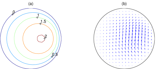
Figure 2: (a) contours of axial velocity $u$ of the viscously dominated Stokes flow in a helical pipe with curvature $\kappa=0.8$ (chosen so large to accentuate the modifications); (b) corresponding torsion induced cross-pipe fluid velocities to leading order in the torsion. The plots are evaluated from the asymptotic solution with errors ${\cal O}\big{(}\kappa^{5}\big{)}$.

See that, for example, the Stokes flow in a torus ($\kappa=\mbox{const}$ and $\tau=0$) is simply one of axial flow, see Figure 2(a), in an adjusted mean pressure gradient as all other components vanish. The axial velocity maximum is shifted to the inside of the curve (to the right in Figure 2(a)) and is increased slightly. In contrast to flows at significant Reynolds number, the pressure gradient around a curve is less than that in a straight pipe presumably because the bulk of the fluid travels a shorter path than the centre line—this agrees with Larrain [18] who used computer algebra to also find high order approximations to the flow in a coiled pipe.

The cross-pipe velocities in a helical pipe are indicated in Figure 2(b) where the torsion induces velocities proportional to those shown in the figure; the generally upwards velocity matching the upwards twist of positive torsion. Observe that torsion, $\tau$, and variations in curvature, $\kappa^{\prime}$, only affect the cross-stream velocities and do not influence the axial velocity $u$ to this order. Conversely, observe that this Stokes flow does not have cross-pipe circulation—the strong viscosity eliminates inertia. Instead the curvature of the pipe just skews and alters the velocity field. For curvature $\kappa\neq 0$ the maximum of the axial velocity $u$ increases and moves towards the inner wall of the pipe. This last effect, though seemingly small even for the large curvature of $\kappa=0.8$ used in Figure 2, is enough to have a strong influence on the shear dispersion as seen in (5).

2.3 Laminar flow at finite Reynolds number

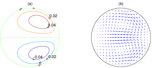
Figure 3: (a) axial velocity $u$ contours of the inertial corrections to Poiseuille flow in a helical pipe with curvature $\kappa=0.5$ to leading order in the torsion $\tau$ of the helix; (b) corresponding inertia induced cross-pipe fluid velocities independent of the torsion. The plots are evaluated from an asymptotic solution with errors ${\cal O}\big{(}\kappa^{5}\big{)}$.

Incorporating the terms representing the advection of fluid momentum into the computer algebra program of Appendix A leads to effects parametrised by the Reynolds number ${\cal R}$. I find that the fluid fields given previously in (15–19) are modified by the addition of the following terms:

$$u = \cdots+\frac{{\cal R}}{144}r\left(1-r^{2}\right)\left(29+5r^{2}-3r^{4}\right)\left[\cos\theta\,\kappa^{\prime}+\sin\theta\,\kappa\tau\right]$$ (20)

$${}-\frac{{\cal R}^{2}}{1440}r\left(1-r^{2}\right)\left(19-21r^{2}+9r^{4}-r^{6}\right)\cos\theta\,\kappa$$

$${}+\frac{{\cal R}^{3}}{1814400}r\left(1-r^{2}\right)\left(2969-4381r^{2}+3249r^{4}-1301r^{6}\right.$$

$$\left.\quad{}+274r^{8}-20r^{10}\right)\left[\cos\theta\,\kappa^{\prime}+\sin\theta\,\kappa\tau\right]+{\cal O}\big{(}\kappa^{2},\delta^{2}\big{)}\,,$$

$$v = \cdots-\frac{{\cal R}}{72}\left(1-r^{2}\right)^{2}\left(4-r^{2}\right)\cos\theta\,\kappa$$ (21)

$${}+\frac{{\cal R}^{2}}{8640}\left(1-r^{2}\right)^{2}\left(13-15r^{2}+7r^{4}-r^{6}\right)\left[\cos\theta\,\kappa^{\prime}+\sin\theta\,\kappa\tau\right]$$

$${}+{\cal O}\big{(}\kappa^{2},\delta^{2}\big{)}\,,$$

$$w = \cdots+\frac{{\cal R}}{72}\left(1-r^{2}\right)\left(4-23r^{2}+7r^{4}\right)\sin\theta\,\kappa$$ (22)

$${}+\frac{{\cal R}^{2}}{8640}\left(1-r^{2}\right)\left(13-224r^{2}+266r^{4}-124r^{6}\right.$$

$$\left.\quad{}+17r^{8}\right)\left[-\sin\theta\,\kappa^{\prime}+\cos\theta\,\kappa\tau\right]+{\cal O}\big{(}\kappa^{2},\delta^{2}\big{)}\,,$$

$$p = \cdots-\frac{{\cal R}}{3}r\left(9-6r^{2}+2r^{4}\right)\cos\theta\,\kappa$$ (23)

$${}+\frac{{\cal R}^{2}}{2160}r\left(101-120r^{2}+90r^{4}-30r^{6}+3r^{8}\right)\left[\cos\theta\,\kappa^{\prime}+\sin\theta\,\kappa\tau\right]$$

$${}+{\cal O}\big{(}\kappa^{2},\delta^{2}\big{)}\,,$$

where “$\cdots$” denote the terms already given for Stokes flow in (15–19). The modifications to the cross-pipe velocities that are proportional to ${\cal R}\kappa(={\mathfrak{D}}^{2}/4{\cal R})$, plotted in Figure 3, agree with those of the Dean flow as used by Johnson [14, p330], in their work on dispersion. The cross-pipe velocity field exhibits circulation across the pipe induced by the pipe curvature because of fluid inertia. The term in the axial velocity $u$ proportional to $\kappa{\cal R}^{2}={\mathfrak{D}}^{2}/4$ also agrees with that of Johnson & Kamm. These terms in the velocity fields are those previously found for the “loosely coiled limit” [3, p467] when curvature $\kappa$ is negligible by itself but the Dean number ${\mathfrak{D}}=2\sqrt{\kappa}{\cal R}$ is significant. The above expressions appear to agree precisely with the expressions (58–61) carefully obtained by Tuttle [34] for low Reynolds number flow in a helical pipe—the only differences lie in various factors of two due to the different non-dimensionalisation and because my angular velocity $w$ is in a “space-centred” coordinate system whereas Tuttle’s $\Phi$ is “body centred”. Lastly, the components of the physical fields (15–23) involving $\sin\theta$ and $\cos\theta$ cross-sectional structures agree with those of Hammack & Hydon [11, p363], but their formulae have none of the components in $\sin 2\theta$, $\cos 2\theta$, nor a modification to the mean pressure gradient as in (24). Observe in all of the formulae (16–23) that torsion coupled to curvature, $\kappa\tau$, appears to have the same effect as longitudinal gradients of curvature, $\kappa^{\prime}$, but the fluid fields are rotated in angle by $90^{\circ}$. The above expressions are the first to combine torsion and general variations in curvature.

With fixed fluid flux, the mean pressure gradient, to one higher order in curvature than the fields above, is

$${\bar{p}}^{\prime} = -8+\left({\textstyle\frac{1}{6}}-{\textstyle\frac{11}{540}}{\cal R}^{2}-{\textstyle\frac{1541}{32659200}}{\cal R}^{4}\right)\kappa^{2}$$ (24)

$${}\quad+\left({\textstyle\frac{23}{80}}{\cal R}+{\textstyle\frac{1433}{241920}}{\cal R}^{3}+{\textstyle\frac{6191}{410572800}}{\cal R}^{5}\right)\kappa\kappa^{\prime}+{\cal O}\big{(}\kappa^{3},\delta^{2}\big{)}\,.$$

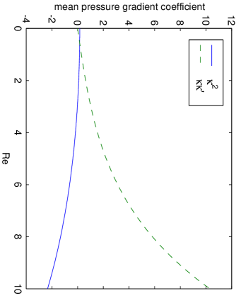
Figure 4: coefficients in the expression (24) for the mean pressure gradient as a function of the centreline curvature $\kappa$ and its gradient $\kappa^{\prime}$.

See from the coefficients plotted in Figure 4, that although the pressure gradient is lessened by curvature for low Reynolds number, for Reynolds number approximately ${\cal R}>3$ there is an increased pressure gradient loss in a curving pipe. This is attributed to the greater mixing caused by the induced cross-pipe circulation. Also see that a region of tightening curvature, increasing $\kappa^{2}$, has a lesser drop in pressure gradient relative to that for a toroidal pipe, whereas conversely a lessening in the curvature, decreasing $\kappa^{2}$, has a higher drop in the pressure gradient. This effect is interpreted as a “memory” in the mean pressure gradient of the upstream conditions: retaining just the highest order terms in ${\cal R}$ the mean pressure gradient

$${\bar{p}}^{\prime} \approx -8-{\textstyle\frac{1541}{32659200}}{\cal R}^{4}\kappa^{2}+{\textstyle\frac{6191}{821145600}}{\cal R}^{5}2\kappa\kappa^{\prime}$$ (25)

$$\approx -8-{\textstyle\frac{1541}{32659200\times 16}}\left.{\mathfrak{D}}^{4}\right|_{s-{4337}{\cal R}/{271216}}\,,$$

where the evaluation of the Dean number at an effective distance upstream of approximately ${\cal R}/6$ pipe radii seems to show the typical distance necessary for the fluid flow to develop in order to accord with the curvature of the pipe. This agrees qualitatively with experiments on a pipe with a finite bend as discussed by Berger et al. [3, p494], where the influence of the bend on the mean pressure gradient extends far downstream. This upstream memory also matches nicely with the commonly quoted distance, $l_{s}\approx\frac{1}{4}a{\cal R}$ [10] and [3, p488], required for flow entering a straight pipe to become fully developed, and with the observation by Murata [22, §4], that the flow in a sinusoidally bent pipe has a lag in its adaptation to the local conditions, the lag increasing with increasing Reynolds number.

The above formulae for both viscous and inertia effects of curvature and torsion are only of low-order. Computer algebra computes the velocity field to as high an order as is necessary for the demands of modelling the dispersion in the pipe, described in the next section. Van Dyke [3, p475] has shown the asymptotic expansions of the fluid flow field converge for Dean number ${\mathfrak{D}}<96.8/4\sqrt{2}=17.1$ (for negligible $\kappa$ but finite ${\mathfrak{D}}$). However, I have not explored this issue as here we are primarily concerned with the advection-diffusion model (2) of the dispersion and its asymptotic approximations.

3 Advection-dispersion along the curving pipe

Having determined the fluid flow within the pipe, I now address the advection and longitudinal dispersion within the pipe. We solve the advection-diffusion equation (2) for the evolving concentration $c(s,r,\vartheta,t)$ of contaminant within the fluid. Writing the concentration in terms of the cross-pipe average $C(s,t)$ and its derivatives I use centre manifold techniques to construct the Taylor model (4), and its higher order generalisations, of the advection-dispersion in the bent and twisted pipe.

3.1 The concentration field within the pipe

Using the coordinate system described in §2.1, the advection-diffusion equation (2) for the evolution of the concentration of the contaminant is

$$\frac{\partial c}{\partial t}+{\cal P}\left(\frac{u}{h_{s}}\frac{\partial c}{\partial s}+v\frac{\partial c}{\partial r}+\frac{w}{r}\frac{\partial c}{\partial\vartheta}\right)$$

$$=\frac{1}{rh_{s}}\left[\frac{\partial}{\partial s}\left(\frac{r}{h_{s}}\frac{\partial c}{\partial s}\right)+\frac{\partial}{\partial r}\left(rh_{s}\frac{\partial c}{\partial r}\right)+\frac{\partial}{\partial\vartheta}\left(\frac{h_{s}}{r}\frac{\partial c}{\partial\vartheta}\right)\right]\,.$$ (26)

This is solved with no flux through the circular walls of the pipe: $\partial c/\partial r=0$ on $r=1$ .

The computer algebra program (Appendix A) simultaneously determines from the contaminant conservation equation (26) the dynamics on the low-dimensional centre manifold, namely the Taylor model (4). Over a cross-pipe diffusion time the concentration field evolves to be, for example, approximately

$$c = C-{\cal P}\frac{\partial C}{\partial s}\frac{1}{24}\left(2-6r^{2}+3r^{4}\right)+{\cal P}\frac{\partial C}{\partial s}\kappa\cos\theta\,\left[-\frac{1}{6}\left(4r-3r^{3}+r^{5}\right)\right.$$ (27)

$$\quad\left.\quad{}+\frac{{\cal R}^{2}}{172800}\left(256r-285r^{3}+200r^{5}-75r^{7}+15r^{9}-r^{11}\right)\right.$$

$$\quad\left.\quad{}+\frac{\sigma{\cal R}^{2}}{34560}\left(68r-120r^{3}+130r^{5}-75r^{7}+21r^{9}-2r^{11}\right)\right]$$

$$\quad{}+{\cal O}\big{(}\kappa^{2},\delta^{2}\big{)}\,.$$

To this order neither torsion nor gradients of curvature affect the concentration field within the pipe, but this is not surprising as one order of $\delta$ is counted in $\partial C/\partial s$ leaving no scope for derivatives of the curvature $\kappa$ to be involved in the above terms. Expressions for the concentration field to the next order in either the curvature $\kappa$ or longitudinal derivatives $\delta$ are algebraically formidable and are not recorded.

From such expressions, the computer algebra determines the mean flux of contaminant through a cross-section of the pipe:

$$F(C,s)=\overline{uc-\frac{1}{h_{s}}\frac{\partial c}{\partial s}}\,,$$

where the overbar denotes the average over a cross-section. Then by conservation of contaminant, the model for the evolution of the contaminant is known to follow $C_{t}=-F_{s}$ . Using the flux $F$ like this I determine the right-hand side of the model to one order higher in axial derivatives, $\delta$, than would otherwise be possible.

3.2 Arbitrary curvature causes upstream memory

The error of ${\cal O}\big{(}\delta\big{)}$ in the shear dispersion coefficient given by (5) encompasses modifications due to both torsion $\tau$ and to variations along the pipe in the curvature $\kappa$. The torsion only affects the dispersion coefficient at ${\cal O}\big{(}\kappa^{2}\tau^{2}\big{)}$ and so does not show up in (5).

Variations in curvature along the pipe ($\kappa^{\prime}\neq 0$) cause the effective dispersion coefficient to become, using ${\mathfrak{R}}$ to denote the scaled Reynolds number ${\cal R}/10$ and remembering ${\cal P}={\cal R}\sigma$,

$$D \!\!\!=\!\!\! 1+\frac{1}{4}\kappa^{2}+\frac{7}{48}\left(\kappa\kappa^{\prime}\right)^{\prime}-\frac{7}{96}\left(\kappa^{2}\tau^{2}+{\kappa^{\prime}}^{2}\right)$$ (28e)

$${}+\frac{{\cal P}^{2}}{48}\left[1+\kappa^{2}\left(-{\textstyle\frac{64225}{171072}}{\mathfrak{R}}^{4}\sigma^{2}+{\textstyle\frac{2995}{24192}}{\mathfrak{R}}^{4}-{\textstyle\frac{36335}{12096}}{\mathfrak{R}}^{2}+{\textstyle\frac{863}{120}}\right)\right]$$

$${}+{\cal P}\kappa\kappa^{\prime}\left[{\mathfrak{R}}^{6}\left({\textstyle\frac{9050586625}{26900729856}}\sigma^{4}+{\textstyle\frac{246093875}{1630347264}}\sigma^{3}-{\textstyle\frac{6234774125}{53801459712}}\sigma^{2}-{\textstyle\frac{1760495125}{40351094784}}\sigma\right)\right.$$

$$\quad\left.{}+{\mathfrak{R}}^{4}\left(-{\textstyle\frac{1068925}{2322432}}\sigma^{3}+{\textstyle\frac{33738035}{20901888}}\sigma^{2}+{\textstyle\frac{2310385}{4478976}}\sigma\right)\right.$$

$$\quad\left.{}+{\mathfrak{R}}^{2}\left(-{\textstyle\frac{383695}{96768}}\sigma^{2}+{\textstyle\frac{19465}{12096}}\sigma+{\textstyle\frac{985}{12096}}\right)\right.$$

$$\quad\left.{}-{\textstyle\frac{13}{32}}\right]$$

$$+{\cal P}^{2}(\kappa^{2}\tau^{2}+{\kappa^{\prime}}^{2})\left[{\mathfrak{R}}^{6}\left({\textstyle\frac{2542365125}{58692501504}}\sigma^{4}-{\textstyle\frac{1039029345155}{126541033242624}}\sigma^{2}-{\textstyle\frac{5542735225}{3515028701184}}\right)\right.$$

$$\quad\left.{}+{\mathfrak{R}}^{4}\left({\textstyle\frac{14791164485}{33108590592}}\sigma^{2}+{\textstyle\frac{739414405}{11036196864}}\right)\right.$$

$$\quad\left.{}+{\mathfrak{R}}^{2}\left(-{\textstyle\frac{7181}{9072}}\sigma^{2}+{\textstyle\frac{7619671}{41803776}}\right)\right.$$

$$\quad\left.{}-{\textstyle\frac{5357}{55296}}\right]$$

$$+{\cal P}{\mathfrak{R}}(\kappa\kappa^{\prime})^{\prime}\left[{\mathfrak{R}}^{6}\left(-{\textstyle\frac{2219783253125}{3012881743872}}\sigma^{5}-{\textstyle\frac{3007270625375}{9038645231616}}\sigma^{4}+{\textstyle\frac{7670650920025}{63270516621312}}\sigma^{3}\right.\right.$$

$$\qquad\left.\left.{}+{\textstyle\frac{2879131496575}{23726443732992}}\sigma^{2}+{\textstyle\frac{396673566125}{15817629155328}}\sigma\right)\right.$$

$$\quad\left.{}+{\mathfrak{R}}^{4}\left({\textstyle\frac{318184675}{306561024}}\sigma^{4}-{\textstyle\frac{3159503125}{752467968}}\sigma^{3}-{\textstyle\frac{9765145925}{16554295296}}\sigma^{2}-{\textstyle\frac{2663242675}{5518098432}}\sigma\right)\right.$$

$$\quad\left.{}+{\mathfrak{R}}^{2}\left({\textstyle\frac{40508065}{4644864}}\sigma^{3}-{\textstyle\frac{3081595}{1548288}}\sigma^{2}-{\textstyle\frac{3844625}{2612736}}\sigma-{\textstyle\frac{16835}{373248}}\right)\right.$$

$$\quad\left.{}+{\textstyle\frac{32413}{27648}}\sigma-{\textstyle\frac{191}{1728}}\right]+{\cal O}\big{(}\kappa^{4},\delta^{3}\big{)}\,,$$

In this large but comprehensive expression observe:

(28e)

gives the molecular diffusivity along the pipe in the presence of the bending and twisting of the pipe when there is no flow;

(28e)

gives the usual shear enhanced dispersion in a straight pipe, ${\cal P}^{2}/48$, modified by the leading order (quadratic) effects of pipe curvature (these were the terms of the shear dispersion discussed in the Introduction (5);

(28e)

gives the leading order effects on the dispersion due to variations in curvature along the pipe;

(28e)

gives the leading order effect of torsion on the dispersion, namely quadratic but moderated by the multiplication by $\kappa^{2}$;

(28e–28e)

through ${\kappa^{\prime}}^{2}$ and $\kappa^{\prime\prime}$ terms, gives the second order effects of the variations in curvature.

It is intriguing to see that the effects of torsion and second order gradients of curvature factorise as shown in (28e–28e). I suggest the reason for this factorisation is due to two effects: firstly, upstream “memory” of the dispersion, to be discussed later, involves

$$\left.\kappa^{2}\right|_{s-\xi}=\kappa^{2}-2\xi\kappa\kappa^{\prime}+\xi^{2}(\kappa\kappa^{\prime})^{\prime}+{\cal O}\big{(}\xi^{3}\big{)}$$

which may explain the appearance of the combination $(\kappa\kappa^{\prime})^{\prime}$; and secondly, curvature gradients and torsion, $\kappa^{\prime}$ and $\kappa\tau$ respectively, both create the same but orthogonal structures in the fluid flow as commented after (20–23).

For large Schmidt number $\sigma$

(typical for material dispersion in liquids) there are two distinguished limits of the above expression for the effective dispersion coefficient, the second being a subset of the first.

• Firstly, for large Schmidt number $\sigma$ the highest powers of $\sigma$ dominate. However, in various subexpressions they appear in combination with the Reynolds number ${\cal R}=10{\mathfrak{R}}$. Thus there is a distinguished limit with large $\sigma$ and small ${\cal R}$ in which ${\cal R}^{2}\sigma$ is of order $1$ . In terms of the magnitude $\delta$ of the slow axial variations, an appropriate scaling is that the fluid flow is slow, ${\cal R}\sim\delta$, the Schmidt number large enough, $\sigma\sim 1/\delta^{2}$, so that the Peclet number is also large, ${\cal P}\sim 1/\delta$, then the effective diffusion coefficient is large, $D\sim 1/\delta^{2}$. Using these orders of magnitude, introducing the order $1$ parameter $\alpha={\cal R}{\cal P}/100={\cal R}^{2}\sigma/100$ and evaluating fractions, the leading order terms in the dispersion coefficient (28) are

  $$D \!\!\!\approx\!\!\! .02083\,{\cal P}^{2}+(.1498-.007821\,\alpha^{2}){\cal P}^{2}\kappa^{2}$$ (29)

  $${}+(-.03965-.004603\,\alpha+.003364\,\alpha^{2}){\cal P}^{3}\kappa\kappa^{\prime}$$

  $${}+(-.007916+.0004332\,\alpha^{2}){\cal P}^{4}(\kappa^{2}\tau^{2}+{\kappa^{\prime}}^{2})$$

  $${}+(.008721+.001038\,\alpha-.0007368\,\alpha^{2}){\cal P}^{4}(\kappa\kappa^{\prime})^{\prime}\,.$$

• Secondly, for a typical Schmidt number $\sigma$ bigger than $10^{3}$ or so, and for any flow with Reynolds number ${\cal R}$ bigger than about $1$, then the parameter $\alpha$ will be bigger than about $10$ and the above expression (29) will be dominated by the quadratic powers in $\alpha$. That is, the dispersion coefficient

  $${D} \!\!\!\approx\!\!\! \left(\frac{{\cal P}}{10}\right)^{2}\left\{2.083+\left(\frac{{\cal R}^{2}\sigma}{100}\right)^{2}\left[-0.7821\,\kappa^{2}+3.364\,\frac{{\cal P}}{10}\kappa\kappa^{\prime}\vphantom{\left(\frac{{\cal P}}{10}\right)^{2}}\right.\right.$$ (30)

  $$\left.\left.{}+\left(\frac{{\cal P}}{10}\right)^{2}\left(4.332\,(\kappa^{2}\tau^{2}+{\kappa^{\prime}}^{2})-7.368\,(\kappa\kappa^{\prime})^{\prime}\right)\right]\right\}.$$

We noted in (25) that the mean pressure gradient in the fluid flow at any location was appropriate to the curvature some distance upstream. Similar memory effects are seen in the dispersion coefficient. The subexpression $-0.7821\,\kappa^{2}+0.3364\,{\cal P}\kappa\kappa^{\prime}$ appearing in the first line of (30) is equivalent to simply $-0.7821\,\kappa^{2}$ evaluated at a distance $\xi=0.2151\,{\cal P}$ upstream from any particular location. I do not attempt to complicate this memory effect any further by trying to include the second order term $(\kappa\kappa^{\prime})^{\prime}$, as there are a plethora of possibilities, but for the purposes of discussion I assume both $\kappa\kappa^{\prime}$ and $(\kappa\kappa^{\prime})^{\prime}$ terms are attributable to upstream memory. The ratio of the coefficients of $\kappa\kappa^{\prime}$ and $\kappa^{2}$ in (29) similarly quantify the upstream memory for low Reynolds number flows as shown in Figure 5. Such memory effects in shear dispersion in varying channels were first recognised by Smith [29].

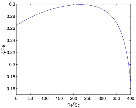
Figure 5: in a generally curving pipe the effective dispersion has the value appropriate to the curvature a distance $\xi$ upstream.

From the coefficient approximations (29) and (30) see that torsion and curvature gradients generally enhance dispersion along the pipe except for low Reynolds numbers, ${\cal R}^{2}\sigma<427.4$ , when they make the dispersion coefficient smaller. However, the effect torsion has upon the dispersion coefficient seems small because not only is the effect quadratic in the torsion $\tau$, it is also ameliorated by the multiplication by the curvature squared. However, ignoring the $\kappa\kappa^{\prime}$ terms and noting that $\kappa^{\prime}=\kappa(\log\kappa)^{\prime}$, I write (30) as

$${D} \!\!\!\approx\!\!\! \left(\frac{{\cal P}}{10}\right)^{2}\left\{2.083\vphantom{\frac{{\cal P}}{10}}\right.$$ (31)

$$\left.{}-0.7821\left(\frac{\kappa{\cal R}^{2}\sigma}{100}\right)^{2}\left[1-\left(\frac{{\cal P}}{10}\right)^{2}5.539\,(\tau^{2}+{(\log\kappa)^{\prime}}^{2})\right]\right\}.$$

This suggests that torsion, or proportional gradients of curvature, greater than about $4/{\cal P}$ may cause the dispersion coefficient $D$ to increase with curvature $\kappa$, instead of decreasing. That torsion could eliminate the increased mixing due to secondary circulations seems unlikely so I predict higher order terms in the torsion $\tau$ would limit its influence on the dispersion.

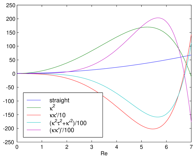
Figure 6: coefficients of the dispersion coefficient $D$ for water at $15^{\circ}\mbox{C}$ given by (32). For higher Reynolds number the highest powers in ${\cal R}$ dominate the coefficients.

For the dispersion of heat in water

with a Prandtl number of $\sigma=8.1$ at $15^{\circ}\mbox{C}$ the dispersion coefficient (28) reduces to

$$D=1.3669\,{\cal R}^{2}+1$$

$${}+\kappa^{2}\left(-.003350\,{\cal R}^{6}-.04106\,{\cal R}^{4}+9.830\,{\cal R}^{2}+.25\right)$$

$${}+\kappa\kappa^{\prime}\left(.01232\,{\cal R}^{7}-.1090\,{\cal R}^{5}-2.01\,{\cal R}^{3}-3.291\,{\cal R}\right)$$

$${}+(\kappa^{2}\tau^{2}+{\kappa^{\prime}}^{2})\left(.01220\,{\cal R}^{8}+.1928\,{\cal R}^{6}-33.95\,{\cal R}^{4}-6.356\,{\cal R}^{2}-.07292\right)$$

$${}+(\kappa\kappa^{\prime})^{\prime}\left(-.02191\,{\cal R}^{8}+.1777\,{\cal R}^{6}+36.39\,{\cal R}^{4}+7.602\,{\cal R}^{2}+.1458\right).$$ (32)

For Reynolds number ${\cal R}>7$ the highest powers in ${\cal R}$ dominate; see Figure 6 for the dependence on smaller ${\cal R}$. Observe: for Reynolds number ${\cal R}>6.95$ curvature enhances the dispersion of heat and vice-versa; whereas for ${\cal R}>6.74$ torsion and curvature gradients reduce the dispersion and vice-versa.

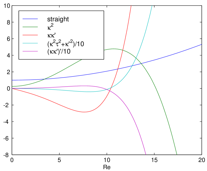
Figure 7: coefficients of the dispersion coefficient $D$ for water at $15^{\circ}\mbox{C}$ given by (33). For higher Reynolds number the highest powers in ${\cal R}$ dominate the coefficients.

For the dispersion of heat in air

with a Prandtl number of $\sigma=0.71$ at $15^{\circ}\mbox{C}$ and recalling that ${\mathfrak{R}}={\cal R}/10$, the dispersion coefficient (28) reduces to

$$D=1.080\,{\mathfrak{R}}^{2}+1$$

$${}+\kappa^{2}\left(-.07649\,{\mathfrak{R}}^{6}-3.244\,{\mathfrak{R}}^{4}+7.767\,{\mathfrak{R}}^{2}+.25\right)$$

$${}+\kappa\kappa^{\prime}\left(.3979\,{\mathfrak{R}}^{7}+7.462\,{\mathfrak{R}}^{5}-5.871\,{\mathfrak{R}}^{3}-2.925\,{\mathfrak{R}}\right)$$

$${}+(\kappa^{2}\tau^{2}+{\kappa^{\prime}}^{2})\left(.3011\,{\mathfrak{R}}^{8}+15.48\,{\mathfrak{R}}^{6}-11.82\,{\mathfrak{R}}^{4}-5.022\,{\mathfrak{R}}^{2}-.07292\right)$$

$${}+(\kappa\kappa^{\prime})^{\prime}\left(-.7615\,{\mathfrak{R}}^{8}-13.98\,{\mathfrak{R}}^{6}+8.055\,{\mathfrak{R}}^{4}+5.282\,{\mathfrak{R}}^{2}+.1458\right)\,.$$ (33)

For Reynolds number ${\cal R}>15$ the highest powers in ${\cal R}$ dominate; see Figure 7 for the dependence on smaller ${\cal R}$. Observe: for Reynolds number ${\cal R}>15.18$ curvature enhances the dispersion of heat and vice-versa; whereas for ${\cal R}>10.35$ torsion and curvature gradients reduce the dispersion and vice-versa.

3.3 Skewness is very sensitive to curvature

Computer algebra straightforwardly determines high order terms in the advection-diffusion equation (2). Chatwin [4] investigated the relatively slow approach to normality in shear dispersion. Here expect the variations in pipe curvature and torsion to distort any normal profile. Hence expect such variations to have a large effect on skewness.

The third order modification to the Taylor model of dispersion is

$$\frac{\partial C}{\partial t}\approx-{\cal P}\frac{\partial C}{\partial s}+\frac{\partial\ }{\partial s}\left(D\frac{\partial C}{\partial s}\right)+\frac{\partial\ }{\partial s}\left(E\frac{\partial^{2}C}{\partial s^{2}}\right)\,,$$ (34)

where the skewness coefficient

$$E \!\!\!=\!\!\! -\frac{{\cal P}^{3}}{2880}$$ (35e)

$${}+{\cal P}\kappa^{2}\left[{\mathfrak{R}}^{6}\left({\textstyle\frac{3241338875}{107602919424}}\sigma^{4}+{\textstyle\frac{1104359125}{35867639808}}\sigma^{2}\right)-{\textstyle\frac{4085615}{20901888}}{\mathfrak{R}}^{4}\sigma^{2}\right.$$

$$\left.\quad{}+{\mathfrak{R}}^{2}\left({\textstyle\frac{68855}{96768}}\sigma^{2}+{\textstyle\frac{985}{12096}}\right)-{\textstyle\frac{13}{32}}\right]$$

$${}+\kappa\kappa^{\prime}\left[{\mathfrak{R}}^{8}\left(-{\textstyle\frac{5943982203125}{9038645231616}}\sigma^{6}-{\textstyle\frac{1183708683125}{2259661307904}}\sigma^{5}-{\textstyle\frac{12012557065375}{9038645231616}}\sigma^{4}\right.\right.$$

$$\left.\left.\qquad{}-{\textstyle\frac{4304114889625}{5931610933248}}\sigma^{3}\right)\right.$$

$$\left.\quad{}+{\mathfrak{R}}^{6}\left({\textstyle\frac{1250362375}{1379524608}}\sigma^{5}+{\textstyle\frac{820657375}{64665216}}\sigma^{4}+{\textstyle\frac{14670875}{4138573824}}\sigma^{3}+{\textstyle\frac{1214048125}{4138573824}}\sigma^{2}\right)\right.$$

$$\left.\quad{}+{\mathfrak{R}}^{4}\left(-{\textstyle\frac{11414525}{290304}}\sigma^{4}+{\textstyle\frac{1917625}{193536}}\sigma^{3}-{\textstyle\frac{25984475}{5225472}}\sigma^{2}-{\textstyle\frac{84175}{93312}}\sigma\right)\right.$$

$$\left.\quad{}+{\mathfrak{R}}^{2}\left({\textstyle\frac{17795}{1152}}\sigma^{2}-{\textstyle\frac{955}{432}}\sigma\right)+{\textstyle\frac{7}{12}}\right]$$

$${}+{\cal P}(\kappa^{2}\tau^{2}+{\kappa^{\prime}}^{2})\left[{\mathfrak{R}}^{8}\left({\textstyle\frac{254564364353125}{1434131710083072}}\sigma^{6}-{\textstyle\frac{9130311425570375}{34419161041993728}}\sigma^{4}\right.\right.$$

$$\left.\left.\qquad{}-{\textstyle\frac{545957180588375}{29041167129182208}}\sigma^{2}\right)\right.$$

$$\left.\quad{}+{\mathfrak{R}}^{6}\left({\textstyle\frac{9773515705025}{2259661307904}}\sigma^{4}+{\textstyle\frac{241252377733475}{759246199455744}}\sigma^{2}\right)\right.$$

$$\left.\quad{}+{\mathfrak{R}}^{4}\left(-{\textstyle\frac{1227346555}{114960384}}\sigma^{4}-{\textstyle\frac{24438946685}{16554295296}}\sigma^{2}-{\textstyle\frac{159535}{2128896}}\right)\right.$$

$$\left.\quad{}+{\mathfrak{R}}^{2}\left({\textstyle\frac{1325215}{258048}}\sigma^{2}-{\textstyle\frac{118243}{580608}}\right)+{\textstyle\frac{801}{2560}}\right]$$

$${}+{\cal P}(\kappa\kappa^{\prime})^{\prime}\left[{\mathfrak{R}}^{8}\left(-{\textstyle\frac{26098554271144375}{206514966251962368}}\sigma^{6}+{\textstyle\frac{10015284615625}{204875958583296}}\sigma^{5}\right.\right.$$

$$\left.\left.\qquad{}+{\textstyle\frac{83884205830882375}{206514966251962368}}\sigma^{4}+{\textstyle\frac{68444215116292625}{464658674066915328}}\sigma^{3}+{\textstyle\frac{44871973001125}{691456360218624}}\sigma^{2}\right)\right.$$

$$\left.\quad{}+{\mathfrak{R}}^{6}\left({\textstyle\frac{71359651375}{6025763487744}}\sigma^{5}-{\textstyle\frac{516258977875}{111588212736}}\sigma^{4}-{\textstyle\frac{596762793925}{2875932573696}}\sigma^{3}\right.\right.$$

$$\left.\left.\qquad{}-{\textstyle\frac{2958969842375}{23007460589568}}\sigma^{2}-{\textstyle\frac{62332574575}{1977203644416}}\sigma\right)\right.$$

$$\left.\quad{}+{\mathfrak{R}}^{4}\left({\textstyle\frac{48287105}{3784704}}\sigma^{4}-{\textstyle\frac{480287515}{172440576}}\sigma^{3}+{\textstyle\frac{4233379915}{2759049216}}\sigma^{2}+{\textstyle\frac{89672375}{459841536}}\sigma+{\textstyle\frac{159535}{2128896}}\right)\right.$$

$$\left.\quad{}+{\mathfrak{R}}^{2}\left(-{\textstyle\frac{23023685}{4644864}}\sigma^{2}+{\textstyle\frac{2964127}{4644864}}\sigma+{\textstyle\frac{501107}{2322432}}\right)-{\textstyle\frac{2257}{5760}}\right]+{\cal O}\big{(}\kappa^{4},\delta^{3}\big{)}\,.$$

The skewness coefficient for flow in a straight pipe, $-{\cal P}^{3}/2880$ from (35e), is well known [5]. One outstanding puzzle in the field of dispersion is that in rivers one observes contaminant concentrations with long tails upstream (not downstream) [2, e.g.]. But theoretical models predict either only a weak enhancement of upstream tails or more confoundedly, as the above negative skewness coefficient implies for straight pipe flow, a weak downstream tail. However, as we now see, curvature effects, presumably induced by the secondary flows, significantly change the skewness coefficient thereby enhancing the upstream tail of a contaminant release. With the caveat that this derivation is for pipes, not rivers, this is a qualitative improvement in the theoretical model compared with observations.

For large Schmidt number $\sigma$

(typical for the dispersion of material in liquids), and similar to the dispersion coefficient $D$, there are two distinguished limits of the above expression for the skewness coefficient.

• Firstly, in terms of the magnitude $\delta$ of the slow axial variations, the appropriate scaling is that the fluid flow is slow, ${\cal R}\sim\delta$, the Schmidt number large enough, $\sigma\sim 1/\delta^{2}$, so that the Peclet number is also large, ${\cal P}\sim 1/\delta$, then the skewness coefficient is large, $E\sim 1/\delta^{3}$. Recalling the parameter $\alpha={\cal R}{\cal P}/100={\cal R}^{2}\sigma/100$ and evaluating fractions, the leading order terms in the skewness coefficient (35) are

  $$E \approx -\frac{{\cal P}^{3}}{2880}\left[1-\kappa^{2}\left(.8675\,\alpha^{2}+20.49\right)\right.$$ (36)

  $$\left.\quad{}+{\cal P}\kappa\kappa^{\prime}\left(.1894\,\alpha^{2}-.2610\,\alpha+11.32\right)\right.$$

  $$\left.\quad{}+{\cal P}^{2}(\kappa^{2}\tau^{2}+{\kappa^{\prime}}^{2})\left(-.05112\,\alpha^{2}+3.075\right)\right.$$

  $$\left.\quad{}+{\cal P}^{2}(\kappa\kappa^{\prime})^{\prime}\left(.03640\,\alpha^{2}-.003411\,\alpha-3.674\right)\right]$$

• Secondly, for a typical Schmidt number $\sigma$ bigger than $10^{3}$ or so, and for any flow with Reynolds number ${\cal R}$ bigger than about $2$, then the parameter $\alpha$ will be bigger than about $40$ and the above skewness coefficient (36) is dominated by the quadratic powers in $\alpha$:

  $${E} \approx \frac{{\cal P}^{3}}{2880}\left\{-1+\left(\frac{{\cal R}^{2}\sigma}{100}\right)^{2}\left[0.8675\,\kappa^{2}-1.894\,\frac{{\cal P}}{10}\kappa\kappa^{\prime}\right.\right.$$ (37)

  $$\left.\left.{}+\left(\frac{{\cal P}}{10}\right)^{2}\left(5.112\,(\kappa^{2}\tau^{2}+{\kappa^{\prime}}^{2})-3.640\,(\kappa\kappa^{\prime})^{\prime}\right)\right]\right\}.$$

  In this regime, even small curvature, through the $\kappa^{2}$ term, will cause the skewness coefficient to become positive, possibly large, and so lead to concentration tails upstream (qualitatively as observed in rivers). Torsion in the pipe leads to the same upstream tails.

Recognise another upstream memory effect. The subexpression $0.8675\,\kappa^{2}-0.1894\,{\cal P}\kappa\kappa^{\prime}$ appearing in the first line of (37) is equivalent to simply $0.8675\,\kappa^{2}$ evaluated at a distance $\xi=0.1092\,{\cal P}$ upstream from any particular location. This upstream memory is approximately half that of the dispersion coefficient.

For the dispersion of heat in water

with a Prandtl number of $\sigma=8.1$ at $15^{\circ}\mbox{C}$ the skewness coefficient (35) reduces to

$$E=-0.1845\,{\cal R}^{3}$$

$${}+\kappa^{2}\left(-3.291\,{\cal R}+3.788\,{\cal R}^{3}-.01039\,{\cal R}^{5}+.001067\,{\cal R}^{7}\right)$$

$${}+\kappa\kappa^{\prime}\left(.5833+9.956\,{\cal R}^{2}-16.43\,{\cal R}^{4}+.08625\,{\cal R}^{6}-.002101\,{\cal R}^{8}\right)$$

$${}+(\kappa^{2}\tau^{2}+{\kappa^{\prime}}^{2})\left(2.534\,{\cal R}+27.28\,{\cal R}^{3}-37.30\,{\cal R}^{5}+.1509\,{\cal R}^{7}+.003968\,{\cal R}^{9}\right)$$

$${}+(\kappa\kappa^{\prime})^{\prime}\left(-3.174\,{\cal R}-25.91\,{\cal R}^{3}+43.37\,{\cal R}^{5}-.1589\,{\cal R}^{7}-.002604\,{\cal R}^{9}\right).$$ (38)

For Reynolds number ${\cal R}>11$ the highest powers in ${\cal R}$ dominate. Observe that for these Reynolds numbers both curvature and torsion may easily reverse the sign of of the skewness paramater $E$ through the combination

$$+{\cal R}^{7}\left[.001067\,\kappa^{2}+.003968\,{\cal R}^{2}(\kappa^{2}\tau^{2}+{\kappa^{\prime}}^{2})\right]\,.$$

Again this effect promotes upstream tails in the dispersion. Although the terms in $\kappa\kappa^{\prime}$ and $(\kappa\kappa^{\prime})^{\prime}$ may keep $E$ negative, we prefer to interpret these as representing upstream memory.

For the dispersion of heat in air

with a Prandtl number of $\sigma=0.71$ at $15^{\circ}\mbox{C}$ and recalling that ${\mathfrak{R}}={\cal R}/10$, the dispersion coefficient (35) reduces to

$$E=-0.1242\,{\mathfrak{R}}^{3}$$

$${}+\kappa^{2}\left(-2.884\,{\mathfrak{R}}+3.124\,{\mathfrak{R}}^{3}-0.6995\,{\mathfrak{R}}^{5}+0.1645\,{\mathfrak{R}}^{7}\right)$$

$${}+\kappa\kappa^{\prime}\left(0.5833+6.217\,{\mathfrak{R}}^{2}-9.592\,{\mathfrak{R}}^{4}+3.537\,{\mathfrak{R}}^{6}-0.7762\,{\mathfrak{R}}^{8}\right)$$

$${}+(\kappa^{2}\tau^{2}+{\kappa^{\prime}}^{2})\left(2.221\,{\mathfrak{R}}+16.93\,{\mathfrak{R}}^{3}-25.07\,{\mathfrak{R}}^{5}+8.940\,{\mathfrak{R}}^{7}-0.3844\,{\mathfrak{R}}^{9}\right)$$

$${}+(\kappa\kappa^{\prime})^{\prime}\left(-2.782\,{\mathfrak{R}}-12.99\,{\mathfrak{R}}^{3}+22.94\,{\mathfrak{R}}^{5}-9.478\,{\mathfrak{R}}^{7}+1.287\,{\mathfrak{R}}^{9}\right)\,.$$ (39)

For Reynolds number ${\cal R}>40$ the highest powers in ${\cal R}$ dominate. Observe that for such larger Reynolds number the sign of the skewness coefficient changes sign sensitively depending upon the torsion $\tau$, curvature $\kappa$, and its gradients.

3.4 Higher order curvature affects the dispersion

Computer algebra also straightforwardly determines even higher order corrections to the dispersion coefficient. These terms may be used, for example, to give estimates of the errors in the earlier approximations. However, the algebraic expressions quickly become extremely complicated. We just extend the analysis to the next order in curvature, but no higher order in gradients, to obtain the following correction to the dispersion coefficient (28):

$$D = \cdots+{\textstyle\frac{1}{8}}\kappa^{4}$$ (40)

$$+\frac{{\cal P}^{2}\kappa^{4}}{48}\left[{\cal R}^{8}\left({\textstyle\frac{6959456407}{3094629863915520000}}\sigma^{4}+{\textstyle\frac{148720297230839}{464658674066915328000000}}\sigma^{2}\right.\right.$$

$$\qquad\left.\left.-{\textstyle\frac{11319036743801}{14297189971289702400000}}\right)\right.$$

$$\quad\left.+{\cal R}^{6}\left({\textstyle\frac{21839753491553}{12654103324262400000}}\sigma^{2}+{\textstyle\frac{1800408289399}{2711593569484800000}}\right)\right.$$

$$\quad\left.+{\cal R}^{4}\left(-{\textstyle\frac{24648813997}{64377815040000}}\sigma^{2}+{\textstyle\frac{5096950451}{21459271680000}}\right)\right.$$

$$\quad\left.-{\textstyle\frac{4685593}{348364800}}{\cal R}^{2}+{\textstyle\frac{13829}{9216}}\right]+{\cal O}\big{(}\kappa^{6},\delta\big{)}\,;$$

or approximately

$$D \approx \cdots+{\textstyle\frac{1}{8}}\kappa^{4}$$ (41)

$${}+\frac{{\cal P}^{2}\kappa^{4}}{48}\left[\left(\frac{{\cal R}}{10}\right)^{8}\left(0.22\sigma^{4}+0.032\sigma^{2}-0.079\right)\right.$$

$$\quad\left.{}+\left(\frac{{\cal R}}{10}\right)^{6}\left(1.7\sigma^{2}+0.66\right)+\left(\frac{{\cal R}}{10}\right)^{4}\left(-3.8\sigma^{2}+2.4\right)\right.$$

$$\quad\left.{}-1.3\left(\frac{{\cal R}}{10}\right)^{2}+1.5\right]+{\cal O}\big{(}\kappa^{6},\delta\big{)}\,.$$

I also computed the dispersion coefficient to the next correction, with errors ${\cal O}\big{(}\kappa^{8},\delta\big{)}$. Then recalling the Dean number ${\mathfrak{D}}=2\sqrt{\kappa}{\cal R}$, the dominant terms for the coefficient of dispersion of material in liquids, large Schmidt number $\sigma$, are:

$$D \approx \frac{{\cal P}^{2}}{48}\left[1-0.3754\left(\frac{{\mathfrak{D}}^{2}\sigma}{400}\right)^{2}+0.2249\left(\frac{{\mathfrak{D}}^{2}\sigma}{400}\right)^{4}-0.1388\left(\frac{{\mathfrak{D}}^{2}\sigma}{400}\right)^{6}\right.$$

$$\left.{}\vphantom{\frac{{\mathfrak{D}}^{2}\sigma}{400}}+{\cal O}\big{(}{\mathfrak{D}}^{16}\sigma^{8}\big{)}\right]\,.$$

This expression is valid for small enough ${\mathfrak{D}}^{2}\sigma$ . Using the additional information [14, §4.3] that the limit at large ${\mathfrak{D}}^{2}\sigma$ is approximately $0.20$ , I construct the following Padé approximant in terms of $\alpha={{\mathfrak{D}}^{2}\sigma}/{400}$

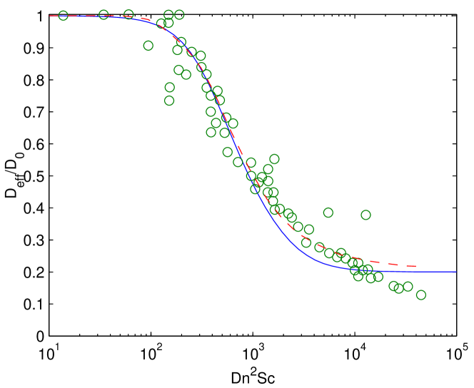
Figure 8: comparison of the Padé approximant (42) (solid) with experimental estimates (circles) collated by Johnson [14], Fig. 9, and the predictions (dashed line) of their spectral method based on Poiseuille flow.

$$D\approx\frac{{\cal P}^{2}}{48}\times\frac{1+0.3068\,\alpha^{2}+0.007811\,\alpha^{4}}{1+0.6822\,\alpha^{2}+0.03905\,\alpha^{4}}\,.$$ (42)

See in Figure 8 that this expression for the dispersion coefficient matches reasonably well with experiments over the whole range of ${\mathfrak{D}}^{2}\sigma$ .

4 Conclusion

Computer algebra handles the considerable details of deriving the complicated expressions describing dispersion in generally curving pipes, §A. Fixing one of the fluid flux or the mean pressure gradient affects the dispersion, §1, and throughout I present results for the appropriate case of fixed fluid flux. The Padé approximation (42) for the dispersion in a constant curvature pipe is reasonably accurate over the entire range of Dean numbers. When the pipe’s curvature and torsion vary, much of the effects of variations upon the dispersion may be recast as an upstream memory. Overall, torsion $\tau$ in the pipe seems to have little effect on the dynamics except for a sensitivity, in combination with the curvature $\kappa$, of the skewness, §3.3. The skewness coefficient is very sensitive to curvature, hence is easily made positive, and which may thus explain the observations of long upstream tails in the dispersion of material in rivers.

Appendix A Computer algebra derivation

Computer algebra is a very powerful means to derive asymptotic expansions. In order for other people to reproduce and verify the results recorded herein, I list here the core of the program used to derive the asymptotic expansions; obtain the full program by request.

The computer algebra program was written in reduce to calculate the asymptotic expansions of the centre manifold models described in this article.

There is a lot of detail to the computer algebra program. However, the key to the correctness of the results is the coding of the governing equations which forms the key part of the core printed here. The algorithm iteratively drives to zero the residuals of these equations, see Roberts [26] for a generic description of the algorithm. Thus the details about how the residuals are reduced are not vital, only that they are correctly computed and ultimately zero.

comment Find the flow in an arbitrarily curving pipe,
Simultaneously determine the shear dispersion in such a flow:
eps=magnitude of curvature terms,
del=magnitude of axial derivatives and of torsion.
;
depend kap,s; % curvature
depend tau,s; % torsion
% local coordinate system is (s,r,th), tp=th+phi(s)
depend tp,s,th;
let { df(tp,s)=>-tau, df(tp,th)=>1 };
hs:=1-eps*kap*r*cos(tp);
hr:=1;
ht:=r;
% trigonometry rules OK
let { sin(~a)*cos(~b) => (sin(a+b)+sin(a-b))/2
    , cos(~a)*cos(~b) => (cos(a-b)+cos(a+b))/2
    , sin(~a)*sin(~b) => (cos(a-b)-cos(a+b))/2
    , cos(~a)^2       => (1+cos(2*a))/2
    , sin(~a)^2       => (1-cos(2*a))/2
    };
% mean over a cross section (mult by r to use)
depend r,rt;depend tp,rt;
operator mean; linear mean;
let { mean(r^~m*cos(~n),rt) => 0
    , mean(r^~m*sin(~n),rt) => 0
    , mean(r^~m,rt) => 2/(m+1)
    , mean(r,rt) => 1
    };
% operators to solve for updates
...
% initial approximations
u:=2*(1-r^2) +eps*3/2*kap*(r-r^3)*cos(tp);
v:=0;
w:=0;
% pressure = ps + p
% = (local mean gradient) + (zero mean fluctuation)
ps:=-8; p:=0;
% concentration of tracer, mean c.
depend c,s,t;
let df(c,t)=>g;
cc:=c;
g:=0;
pe:=re*sc; % Peclet number = Reynolds * Schmidt
rh:=1; % approx reciprocal of axial scale factor hs
% iterate until residuals are negligible
let { eps^3=>0, del^5=>0 }; % truncate the asymptotics
repeat begin
    % reciprocal of scale factor
    eqr:=hs*rh-1;
    rh:=rh-eqr;
    % vorticity
    oms:=(df(r*w,r)-df(v,th))/r;
    omr:=(df(hs*u,th)-del*df(r*w,s))*rh/r;
    omt:=(del*df(v,s)-df(hs*u,r))*rh;
    % Navier-Stokes equation
    nss:=rh*(ps+del*df(p,s)) +(df(r*omt,r)-df(omr,th))/r
        +re*( del*u*df(u,s)*rh+v*df(u,r)+w*df(u,th)/r
             +u*df(hs,r)*v*rh+u*df(hs,th)*w*rh/r );
    nsr:=df(p,r)    +(df(hs*oms,th)-del*df(r*omt,s))*rh/r
        +re*( del*u*df(v,s)*rh+v*df(v,r)+w*df(v,th)/r
             -w^2/r-df(hs,r)*u^2*rh );
    nst:=df(p,th)/r +(del*df(omr,s)-df(hs*oms,r))*rh
        +re*( del*u*df(w,s)*rh+v*df(w,r)+w*df(w,th)/r
             -u^2*df(hs,th)*rh/r+v*w/r );
    % continuity equation
    cty:=(del*df(r*u,s)+df(r*hs*v,r)+df(hs*w,th))*rh/r;
...
    % equation for tracer evolution
    ceq:= df(cc,t) +pe*( del*u*df(cc,s)*rh+v*df(cc,r)+w*df(cc,th)/r )
         -(del^2*df(rh*r*df(cc,s),s)+df(r*hs*df(cc,r),r)
            +df(hs/r*df(cc,th),th))*rh/r;
    cmean:=mean(r*hs*cc,rt)-c;
    ...
end until (eqr=0)and(nss=0)and(nsr=0)and(nst=0)
       and(cty=0)and(ceq=0)and(cmean=0);
% check subsiduary conditions
uwall:=sub(r=1,u);
vwall:=sub(r=1,v);
wwall:=sub(r=1,w);
umean:=mean(r*u,rt);
pmean:=mean(r*p,rt);
cwall:=sub(r=1,df(cc,r));
cflux:=mean(r*(u*pe*cc-del*rh*df(cc,s)),rt);
end;

Observe that the pressure is decomposed into a mean gradient and a cross-pipe fluctuating component. There is code to adjust the mean pressure gradient to ensure a constant mean fluid flux. To adapt to the traditional fixed pressure gradient in a helical or toroidal pipe, one just needs to omit the modifications. However, the results are then inappropriate to a pipe with varying curvature or torsion.

References

- [1] G. K. Batchelor. An Introduction to Fluid Dynamics. CUP, 1979.
- [2] T. Beer and P. C. Toung. Longitudinal dispersion in natural streams. J. Environmental Eng, 109:1049–1067, 1983.
- [3] S. A. Berger, L. Talbot, and L.-S. Yao. Flow in curved pipes. Ann. Rev. Fluid Mech., 15:461–512, 1983.
- [4] P. C. Chatwin. The approach to normality of the concentration distribution of a solute in a solvent flowing along a straight pipe. J. Fluid Mech, 43:321–352, 1970.
- [5] P. C. Chatwin and C. M. Allen. Mathematical models of dispersion in rivers and estuaries. Annu. Rev. Fluid Mech., 17:119–149, 1985.
- [6] P. Daskopoulos and A. M. Lenhoff. Flow in curved ducts: bifurcation structure for stationary ducts. J. Fluid Mech., 203:125–148, 1989.
- [7] W. R. Dean. Note on the motion of fluid in a curved pipe. Phil. Mag., 4:208–223, 1927.
- [8] W. R. Dean. The stream-line motion of fluid in a curved pipe. Phil. Mag., 5:673–695, 1928.
- [9] M. E. Erdogan and P. C. Chatwin. The effects of curvature and buoyancy on the laminar dispersion of solute in a horizontal tube. J. Fluid Mech., 29:465–484, 1967.
- [10] D. Fargie and B. W. Martin. Developing flow in a pipe of circular cross section. Proc. Roy. Soc. Lond. A, 321:461–476, 1971.
- [11] D. Gammack and P. E. Hydon. Flow in pipes with non-uniform curvature and torsion. J. Fluid Mech., 433:357–382, 2001.
- [12] M. Germano. On the effect of torsion on a helical pipe flow. J. Fluid Mech., 125:1–8, 1982.
- [13] Sandip Ghosal. Lubrication theory for electro-osmotic flow in a microfluidic channel of slowly varying cross-section and wall charge. J. Fluid Mech., 459:103–128, 2002.
- [14] M. Johnson and R. D. Kamm. Numerical studies of steady flow dispersion at low Dean number in a gently curving tube. J. Fluid Mech., 172:329–345, 1986.
- [15] S. W. Jones and W. R. Young. Shear dispersion and anomalous diffusion by chaotic advection. J. Fluid Mech., 280:149–172, 1994.
- [16] H. C. Kao. Torsion effects on fully developed flow in a helical pipe. J. Fluid Mech., 184:335–356, 1987.
- [17] E. Kreyszig. Advanced engineering mathematics. Wiley, 8th edition, 1999.
- [18] J. Larrain and C. F. Bonilla. Theoretical analysis of pressure drop in the laminar flow of fluid in a coiled pipe. Trans. Soc. Rheol., 14:135–147, 1970.
- [19] S. Liu and J. Masliyah. Axially invariant laminar flow in helical pipes with finite pitch. J. Fluid Mech., 251:315–353, 1993.
- [20] D. J. McConalogue. The effects of secondary flow on the laminar dispersion of an injected substance in a curved tube. Proc. Roy. Soc. Lond. A, 315:99–113, 1970.
- [21] G. N. Mercer and A. J. Roberts. A complete model of shear dispersion in pipes. Jap. J. Indust. Appl. Math., 11:499–521, 1994.
- [22] S. Murata, Y. Miyake, and T. Inaba. Laminar flow in a curved pipe with varying curvature. J. Fluid Mech., 73:735–752, 1976.
- [23] R. J. Nunge, T.-S. Lin, and W. N. Gill. Laminar dispersion in curved tubes and channels. J. Fluid Mech., 51:363–383, 1972.
- [24] T. J. Pedley. Fluid mechanics of large blood vessels. C.U.P., 1980.
- [25] A. J. Roberts. The application of centre manifold theory to the evolution of systems which vary slowly in space. J. Austral. Math. Soc. B, 29:480–500, 1988.
- [26] A. J. Roberts. Low-dimensional modelling of dynamics via computer algebra. Computer Phys. Comm., 100:215–230, 1997.
- [27] A. J. Roberts. Low-dimensional modelling of dynamical systems applied to some dissipative fluid mechanics. In Rowena Ball and Nail Akhmediev, editors, Nonlinear dynamics from lasers to butterflies, volume 1 of Lecture Notes in Complex Systems, chapter 7, pages 257–313. World Scientific, 2003.
- [28] D. M. Ruthven. The residence time distribution for ideal laminar flow in helical tubes. Chem Eng Sci, 26:1113–1121, 1971.
- [29] R. Smith. Longitudinal dispersion coefficients for varying channels. J. Fluid Mech., 130:299–314, 1983.
- [30] G. I. Taylor. Dispersion of soluble matter in solvent flowing slowly through a tube. Proc. Roy. Soc. Lond. A, 219:186–203, 1953.
- [31] G. I. Taylor. Conditions under which dispersion of a solute in a stream of solvent can be used to measure molecular diffusion. Proc. Roy. Soc. Lond. A, 225:473–477, 1954.
- [32] H. C. Topakoglu. Steady laminar flows of an incompressible viscous fluid in curved pipes. J. Math. Mech., 16:1321–1338, 1967.
- [33] R. N. Trivedi and K. Vasudeva. Axial dispersion in laminar flow in helical coils. Chem Engrg. Sci., 30:317–325, 1975.
- [34] E. R. Tuttle. Laminar flow in twisted pipes. J. Fluid Mech., 219:545–570, 1990.
- [35] S. D. Watt and A. J. Roberts. The construction of zonal models of dispersion in channels via matching centre manifolds. J. Austral. Maths. Soc. B, 38:101–125, 1996.
- [36] K. Yamamoto, S. Yanase, and T. Yoshida. Torsion effect on the flow in a helical pipe. Fluid Dyn. Res., 14:259–273, 1994.
- [37] K. Yamamoto, S. Yanase, and T. Yoshida. Erratum: Torsion effect on the flow in a helical pipe. Fluid Dyn. Res., 24:309–311, 1999.
- [38] L. Zabielski and A. J. Mestel. Steady flow in a helically symmetric pipe. J. Fluid Mech., 370:297–320, 1998.