Traveling solitons in the damped driven nonlinear Schrödinger equation

Abstract

The well known effect of the linear damping on the moving nonlinear Schrödinger soliton (even when there is a supply of energy via the spatially homogeneous driving) is to quench its momentum to zero. Surprisingly, the zero momentum does not necessarily mean zero velocity. We show that two or more parametrically driven damped solitons can form a complex traveling with zero momentum at a nonzero constant speed.

All traveling complexes we have found so far, turned out to be unstable. Thus, the parametric driving is capable of sustaining the uniform motion of damped solitons, but some additional agent is required to stabilize it.

I Introduction

The amplitude of a nearly-harmonic wave propagating in a nonlinear dispersive medium satisfies a nonlinear Schrödinger equation. Confining ourselves to the generic, cubic, nonlinearity of the ‘focusing’ type, the resulting nonlinear Schrödinger equation is of the form

$$i\Psi_{t}+\Psi_{xx}+2|\Psi|^{2}\Psi=-i\gamma\Psi;\quad\gamma>0.$$ (1)

The $-i\gamma\Psi$ term in the right-hand side accounts for dissipative losses (which were assumed to be small in the derivation of eq.(1).) In the underlying physical system the dissipation is compensated by pumping the energy into the system, in one way or another. The pumping is modeled by adding a driving term to the right-hand side of eq.(1).

Like a simple pendulum, the distributed system can be driven externally or parametrically. The typical form of the corresponding amplitude equation is

$$i\Psi_{t}+\Psi_{xx}+2|\Psi|^{2}\Psi=he^{i\Omega t}-i\gamma\Psi,$$ (2)

and

$$i\Psi_{t}+\Psi_{xx}+2|\Psi|^{2}\Psi=h{\overline{\Psi}}e^{2i\Omega t}-i\gamma\Psi,$$ (3)

respectively. (The overline in the right-hand side of (3) indicates complex conjugation.) Both the externally and parametrically driven nonlinear Schrödinger equations arise in a great variety of physical contexts. In particular, the parametric equation (3) describes the nonlinear Faraday resonance in a vertically oscillating water tank Miles ; ElphickMeron1 ; Faraday and the effect of phase-sensitive amplifiers on solitons in optical fibers optics . The same equation controls the magnetization waves in an easy-plane ferromagnet exposed to a combination of a static and microwave field BBK and the amplitude of synchronized oscillations in vertically vibrated pendula lattices pendula .

Both equations (2) and (3) exhibit soliton solutions RoySoc ; Smirnov ; boundary , Miles ; ElphickMeron1 ; BBK , stable and unstable Smirnov ; BBK , which can also form (stable and unstable) multisoliton complexes Malomed ; BSA ; BZ . All localized solutions that have been found so far, were non-propagating. In fact, it is widely accepted that the nonlinear Schrödinger solitons simply cannot travel in the presence of dissipation. This perception is based on the rate equation

$$\dot{P}=-2\gamma P,$$ (4)

which is straightforward from (2) and (3). Here $P$ is the total field momentum,

$$P=\frac{i}{2}\int_{-\infty}^{\infty}(\overline{\Psi}_{x}\Psi-\Psi_{x}\overline{\Psi})dx.$$ (5)

In the undamped case ($\gamma=0$) the momentum is conserved; however if $\gamma>0$, $P$ decays to zero and this seems to suggest that a solitary wave, initially moving with a nonzero velocity, will have to slow down and eventually stop KN_PRB .

Another indication that only quiescent solitons are possible in the damped-driven Schrödinger equation, comes ostensibly from the singular ElphickMeron1 ; ElphickMeron2 and Inverse Scattering-based perturbation theory RoySoc ; KivsharMalomed ; Shesnovich . Here we should mention however that these techniques are well developed only in the one-soliton sector and in the case of several well separated solitons. They either make use of the smallness of the perturbation in the right-hand side of (2)-(3) ElphickMeron1 ; RoySoc ; KivsharMalomed or utilize an explicit form of the perturbed soliton (to study its stability and bifurcation) Shesnovich . In any case, the resulting finite-dimensional system of equations for the parameters of the soliton and radiations, leads to the conclusion that the soliton’s velocity has to decay to zero as $t\to\infty$.

Meanwhile, the moving solitary waves could play a significant role in a variety of physical situations modeled by the damped-driven nonlinear Schrödinger equations. Stable traveling waves could compete with non-propagating localized attractors; unstable ones might arise as long-lived transients and intermediate states in spatiotemporal chaotic regimes. Both types of moving solitary waves could mediate energy dissipation in damped-driven systems. One more reason for not rejecting the unstable solutions outright is their possible persistence within the (directly or parametrically driven) Ginzburg-Landau equations of which the Schrödinger equations (2)-(3) are special cases Ginzburg_Landau . The diffusion and nonlinear damping (the terms $ic_{1}\Psi_{xx}$ and $-ic_{2}|\Psi|^{2n}\Psi$, to be added to the right-hand side of (2)-(3)) are known to have a stabilizing effect on the Ginzburg-Landau pulses; hence the unstable Schrödinger solitons may gain stability as they are continued to nonzero positive $c_{1}$ and $c_{2}$.

The purpose of this paper is to show that the damped-driven nonlinear Schrödinger equations do support solitary waves traveling with nonzero velocities. For the demonstration of this fact we confine our study to the parametrically driven Schrödinger only. The externally driven equation is left as an object of future research.

Two complementary strategies will be pursued to achieve our goal. First, in section III, we consider the motionless damped solitons ($V=0$, $\gamma\neq 0$) and derive the condition under which they can be continued to nonzero velocity. Having identified values of $\gamma$ for which this condition is satisfied, we perform the numerical continuation obtaining a branch of solitary waves with nonzero $V$ and $\gamma$. Our second approach is presented in section IV; the idea is to continue undamped traveling waves ($\gamma=0$, $V\neq 0$) to nonzero dampings. We show that this is only possible if the traveling wave has zero momentum. For complexes with $P=0$, we then carry out the numerical continuation in $\gamma$. In section V we discuss the consistency of results obtained within these two complementary approaches.

We examined, numerically, stability of all solutions obtained within both approaches. The general framework of the stability analysis is outlined in section II. Results of this analysis are presented along with results of the numerical continuation. Finally, section VI summarizes conclusions of our study.

II Mathematical Preliminaries

For purposes of this paper we transform equation (3) to an autonomous form. First, we normalize the driving frequency $\Omega$ to unity; after that, the substitution $\Psi(x,t)=e^{it}\psi(x,t)$ takes eq.(3) to

$$i\psi_{t}+\psi_{xx}+2|\psi|^{2}\psi-\psi=h\overline{\psi}-i\gamma\psi.$$ (6)

This is the representation of the parametrically driven damped nonlinear Schrödinger equation that we are going to work with in this paper. We confine ourselves to uniformly traveling solutions of the form

$$\psi(x,t)=\psi(x-Vt)\equiv\psi(\xi),$$ (7)

where $\psi(\xi)\rightarrow 0$ as $|\xi|\rightarrow\infty$. These satisfy an ordinary differential equation

$$-iV\psi_{\xi}+\psi_{\xi\xi}+2|\psi|^{2}\psi-\psi=h\overline{\psi}-i\gamma\psi.$$ (8)

The analytical part of this paper deals mainly with identifying those of the previously found solutions of (8) with $V=0$ or $\gamma=0$ which can be continued in $V$ and $\gamma$, respectively. The actual continuation will be carried out numerically. Our numerical method employs a predictor-corrector continuation algorithm with a fourth-order accurate Newtonian solver. Typically, the infinite line was approximated by an interval $(-100,100)$. The discretization step size was typically $0.005$. The numerical tolerance was set to be $10^{-10}$; that is, the grid solution would be deemed accurate if the difference between the left- and right-hand sides in (8) were smaller than $10^{-10}$.

Along with the continuation of solutions in $V$ and $\gamma$, we will be analyzing their stability to small perturbations. To this end, we linearize equation eq.(6) in the co-moving frame of reference. Letting $\psi(x,t)=u(\xi)+iv(\xi)+\delta\psi(\xi,t)$, where $u$ and $v$ are the real and imaginary part of the solution that we are linearizing about, and assuming that the linear perturbation depends on time exponentially:

$$\delta\psi(\xi,t)=e^{\lambda t}\left[\delta u(\xi)+i\delta v(\xi)\right],$$

we arrive at an eigenvalue problem

$${\cal H}_{0}\,{\vec{y}}=(\lambda+\gamma)J\,{\vec{y}},$$ (9)

where the operator ${\cal H}_{0}$ is defined by

$${\cal H}_{0}=\left(\begin{array}[]{lr}-\partial_{\xi}^{2}+1+h-6u^{2}-2v^{2}&-V\partial_{\xi}-4uv\\ V\partial_{\xi}-4uv&-\partial_{\xi}^{2}+1-h-6v^{2}-2u^{2}\end{array}\right),$$ (10)

the skew-symmetric matrix $J$ is

$$J=\left(\begin{array}[]{lr}0&-1\\ 1&0\end{array}\right),$$

and the column vector ${\vec{y}}(\xi)=(\delta u,\delta v)^{T}$. The eigenvalue problem (9) was solved by expanding $\delta u$ and $\delta v$ over a Fourier basis, typically with 500 modes, on the interval $(-50,50)$.

The last point that we need to touch upon in this preliminary section, is the integrals of motion of eq.(3), or, more precisely, the quantities which are conserved in the absence of dissipation. When $\gamma=0$, the equation (3) conserves the momentum (given by eq.(5) where one only needs to replace $\Psi\to\psi$), and energy,

$$E=\int_{-\infty}^{\infty}(|\psi_{x}|^{2}+|\psi|^{2}-|\psi|^{4}+h\ {\rm Re}\,\psi^{2})\,dx.$$ (11)

In the damped case, the momentum decays according to the rate equation (4) while the energy satisfies

$$\dot{E}=2\gamma\left(\int_{-\infty}^{\infty}|\psi|^{4}dx-E\right).$$ (12)

III Continuation of damped solitons to nonzero velocities

III.1 Continuability criterion

Our first strategy is to attempt to continue stationary solutions with nonzero $\gamma$ to nonzero $V$. Two basic soliton solutions, denoted $\psi_{+}$ and $\psi_{-}$, are available explicitly:

$$\psi_{\pm}(x)=e^{-i\theta_{\pm}}A_{\pm}\,{\rm sech\/}\left(A_{\pm}x\right);$$ (13)

$$A_{\pm}=\sqrt{1\pm\sqrt{h^{2}-\gamma^{2}}},$$

$$\theta_{+}=\frac{1}{2}\arcsin\frac{\gamma}{h},\quad\theta_{-}=\frac{\pi}{2}-\theta_{+}.$$

The two solitons can form a variety of stationary complexes. These are denoted, symbolically, $\psi_{(++)}$, $\psi_{(--)}$, $\psi_{(+-+)}$, $\psi_{(-+-)}$, and so on BZ . Let $\psi_{0}(x)$ be a particular complex; we want to find out whether it can be continued in $V$. Assuming there is a solution $\psi(\xi;V)$ such that $\psi(\xi;0)\equiv\psi_{0}(\xi)$ $(=\psi_{0}(x))$, we expand $\psi(\xi;V)$ in powers of $V$ as

$$\left.\psi(\xi;V)=e^{-i\theta}\right\{u_{0}(\xi)+iv_{0}(\xi)\left.+V[u_{1}(\xi)+iv_{1}(\xi)]+V^{2}[u_{2}(\xi)+iv_{2}(\xi)]+...\right\},$$ (14)

where the constant phase $\theta$ will be chosen at a later stage. We also expand $h$ and $\gamma$: $h=h_{0}+h_{1}V+...$, $\gamma=\gamma_{0}+\gamma_{1}V+...$. Substituting into (8), the order $V^{1}$ gives

$${\cal L}\left(\begin{array}[]{l}u_{1}\\ v_{1}\end{array}\right)=\left(\begin{array}[]{c}v_{0}^{\prime}\\ -u_{0}^{\prime}\end{array}\right)+{\cal B}\left(\begin{array}[]{c}u_{0}\\ v_{0}\end{array}\right),$$ (15)

where the operator ${\cal L}$ has the form

$${\cal L}=\left(\begin{array}[]{lr}-\partial_{x}^{2}+1+h_{0}\cos 2\theta-6u_{0}^{2}-2v_{0}^{2}&\gamma_{0}+h_{0}\sin 2\theta-4u_{0}v_{0}\\ -\gamma_{0}+h_{0}\sin 2\theta-4u_{0}v_{0}&-\partial_{x}^{2}+1-h_{0}\cos 2\theta-2u_{0}^{2}-6v_{0}^{2}\end{array}\right);$$ (16)

the constant matrix ${\cal B}$ is given by

$${\cal B}=\left(\begin{array}[]{lr}-h_{1}\cos 2\theta&-\gamma_{1}-h_{1}\sin 2\theta\\ \gamma_{1}-h_{1}\sin 2\theta&h_{1}\cos 2\theta\end{array}\right),$$

and the primes over $u_{0}$ and $v_{0}$ indicate derivatives with respect to $x$. (In (15) and (16) we have replaced $\xi$ with $x$ as $\xi$ coincides with $x$ for $V=0$.) According to Fredholm’s alternative, eq.(15) has a bounded solution $u_{1}(x),v_{1}(x)$ iff the vector in the right-hand side is orthogonal to the kernel of the Hermitean-conjugate operator ${\cal L}^{\dagger}$:

$$\int(y,w)\,\left(\begin{array}[]{c}v_{0}^{\prime}\\ -u_{0}^{\prime}\end{array}\right)dx+\int(y,w)\,{\cal B}\left(\begin{array}[]{c}u_{0}\\ v_{0}\end{array}\right)dx=0.$$ (17)

Here ${\vec{y}}(x)=(y,w)^{T}$ is the eigenvector of ${\cal L}^{\dagger}$ associated with the zero eigenvalue: ${\cal L}^{\dagger}{\vec{y}}=0$. That the operator ${\cal L}^{\dagger}$ has a zero eigenvalue follows from the fact that the operator ${\cal L}$ has one — namely, the translation eigenvalue corresponding to the eigenvector $(u_{0}^{\prime},v_{0}^{\prime})^{T}$. Eq.(17) gives a necessary continuability condition of damped quiescent solitons to nonzero velocities.

III.2 Noncontinuability of the ‘building blocks’

It is quite easy to check that when $\gamma_{0}\neq 0$, the individual $\psi_{+}$ and $\psi_{-}$ solitons (the basic ‘building blocks’ of which all complexes are constructed) are not continuable to nonzero $V$. Choosing $\theta=\theta_{+}$ for the $\psi_{+}$ soliton and $\theta=\theta_{-}$ for the $\psi_{-}$ (where $\theta_{\pm}$ are to be computed from the bottom formula in (13) with $\gamma=\gamma_{0}$ and $h=h_{0}$), we get $v_{0}(x)=0$, $\gamma_{0}-h_{0}\sin 2\theta=0$ and so the $2\times 2$ matrix ${\cal L}$, eq.(16), becomes upper triangular. The zero mode of ${\cal L}^{\dagger}$ can now be readily found.

Consider, for instance, the $\psi^{+}$ case. The zero mode satisfies

$$\left(\begin{array}[]{lr}-\partial_{x}^{2}+A_{+}^{2}-6u_{0}^{2}&0\\ 2\gamma_{0}&-\partial_{x}^{2}+A_{-}^{2}-2u_{0}^{2}\end{array}\right)\left(\begin{array}[]{c}y\\ w\end{array}\right)=0,$$

hence $y(x)=u_{0}^{\prime}(x)$ and $w(x)$ is found from

$$(-\partial_{x}^{2}+A_{-}^{2}-2u_{0}^{2})w=-2\gamma u_{0}^{\prime}(x).$$ (18)

Using the explicit expression for $u_{0}(x)$, $u_{0}(x)=A_{+}{\rm sech\/}(A_{+}x)$, the operator in the left-hand side of (18) can be written as $A_{+}^{2}(L_{0}-\epsilon)$, where $\epsilon=2h_{0}\cos(2\theta_{+})/A_{+}^{2}$; $L_{0}$ is given by

$$L_{0}=-\partial_{X}^{2}+1-2{\rm sech\/}^{2}X,$$

and $X=A_{+}x$. The operator $L_{0}$ has familiar spectral properties; in particular it has a single discrete eigenvalue $E_{0}=0$ associated with an even eigenfunction $z_{0}={\rm sech\/}X$, while its continuous spectrum occupies the semi-axis $E_{k}\geq 1$. Consequently, for $0<\epsilon<1$ (that is, for $h_{0}<\sqrt{1+\gamma_{0}^{2}}$), the operator $L_{0}-\epsilon$ is invertible and a bounded solution $w(x)$ of (18) exists and is unique. It can be found explicitly, but this is not really necessary for our purposes. All we need to know is that, since $L_{0}$ is a parity-preserving operator, $w(x)$ has the same parity as the right-hand side in (18), i.e. it is an odd function. For that reason the second integral in equation (17) vanishes and the necessary continuability condition reduces to

$$\gamma\int u_{0}^{\prime}(x)(L_{0}-\epsilon)^{-1}u_{0}^{\prime}(x)dx=0.$$ (19)

This quadratic form can be easily evaluated by expanding $u_{0}^{\prime}(x)$ over eigenfunctions of the operator $L_{0}$:

$$u_{0}^{\prime}(x)=\int_{-\infty}^{\infty}U(k)z_{k}(X)dk,$$

where $L_{0}z_{k}(X)=(1+k^{2})z_{k}(X)$. (The ‘discrete’ eigenfunction $z_{0}(X)$ does not appear in the expansion as it has the opposite parity to $u_{0}^{\prime}(x)$.) Utilizing the orthonormality of the eigenfunctions, the continuability condition (19) is transformed into

$$\gamma\int\frac{|U(k)|^{2}}{k^{2}+1-\epsilon}dk=0.$$ (20)

As $\epsilon<1$, this condition can obviously not be satisfied (unless $\gamma=0$).

In the case of the $\psi_{-}$ soliton the analysis is similar. In this case the continuability condition (20) is replaced by

$$\gamma\int\frac{|U(k)|^{2}}{k^{2}+(1-\epsilon)^{-1}}dk=0,$$

and this cannot be met for the same reason as eq.(20).

III.3 Continuation of the complexes

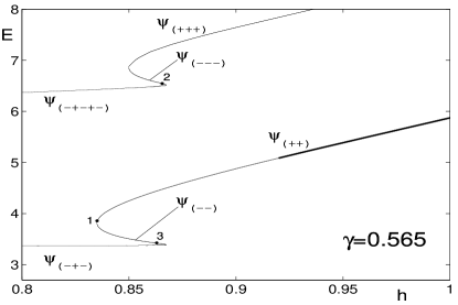
Figure 1: A fragment of the bifurcation diagram for stationary multisoliton complexes (adapted from BZ .) Shown is the energy (11) of the complex as a function of $h$. The bottom branch pertains to symmetric two-soliton complexes $\psi_{(++)}$ and $\psi_{(--)}$ and a three-soliton solution $\psi_{(-+-)}$; the top branch includes the three-soliton states $\psi_{(+++)}$ and $\psi_{(---)}$, as well as a five-soliton solution $\psi_{(-+-+-)}$. The thick curve corresponds to stable and thin curves to unstable solutions. The black dots indicate points where the integral (21) equals zero and therefore moving solitons are allowed to bifurcate off.

Turning to the complexes of the solitons $\psi_{+}$ and $\psi_{-}$, the phase of the complex varies with $x$ and therefore the matrix ${\cal L}$ cannot be made triangular no matter how we choose the constant $\theta$ in (14). For this reason, aggravated by the fact that the multisoliton solutions are not available explicitly, the continuability condition (17) cannot be verified analytically. Resorting to the help of computer, we evaluated the eigenfunction ${\vec{y}}(x)$ associated with the zero eigenvalue of the operator ${\cal L}^{\dagger}$ numerically. (Here we set $\theta=\theta_{+}$).

All damped soliton complexes found in BZ , were symmetric; that is, the corresponding $u$ and $v$ are even functions of $x$. Therefore, the operator ${\cal L}^{\dagger}$ whose potential part is made up of $u(x)$ and $v(x)$, is parity preserving and all its eigenfunctions pertaining to non-repeated eigenvalues are either even or odd. As we move along a continuous branch of solutions, the parity of the eigenfunction has to change continuously. Since the parity equals either $+1$ (for even functions) or $-1$ (for odd functions), the only opportunity left to it by the continuity argument, is to remain constant on the entire branch. For that reason it is sufficient to determine the parity of the eigenfunction for one specific value of $h$ — and we will know it at all other points. Our numerical calculation shows that the eigenfunction ${\vec{y}}(x)$ is odd on all branches reported in BZ . Consequently, the second term in (17) is always zero and we only need to evaluate the first term.

The vanishing of the term involving coefficients $h_{1}$ and $\gamma_{1}$ in eq.(17) implies that it was not really necessary to expand $h$ and $\gamma$ in powers of $V$. This fact has a simple geometric interpretation. As we will see below, for the fixed $\gamma$ the continuable solutions occur only at isolated values of $h$; hence they exist only for $h$ and $\gamma$ lying on continuous curves in the $(h,\gamma)$-plane. Each curve results from an intersection of some surface in the three-dimensional $(h,\gamma,V)$-space and the $V=0$-plane. The fact that one does not have to alter $h$ and $\gamma$ when continuing the solution to nonzero $V$, indicates that these surfaces are orthogonal to the $V=0$ plane along their curves of intersection.

Having found the solution $\psi(x)=u(x)+iv(x)$ at representative points along each branch, we obtained the eigenfunction ${\vec{y}}(x)$ at these points and evaluated what remains of the integral (17):

$$\int(yv_{0}^{\prime}-wu_{0}^{\prime})\,dx\equiv I(h).$$ (21)

The integral $I$ is a continuous function of $h$, and it was not difficult to find points on the curve at which it changes from positive to negative values, or vice versa.

We examined two branches of multisoliton solutions obtained previously BZ (Fig.1). The integral $I(h)$ was found to change its sign at three points, marked by black dots in Fig.1. (Although it may seem from the figure that $I$ equals zero right at the turning points, in the actual fact zeros of $I$ do not exactly coincide with the turning points.) We were indeed able to numerically continue our solutions in $V$ from each of these three points. Results are presented in Fig.2, (a)-(c).

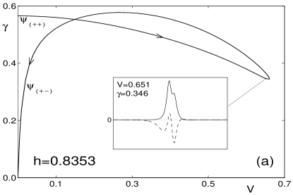
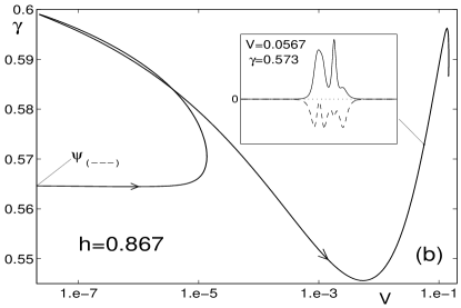
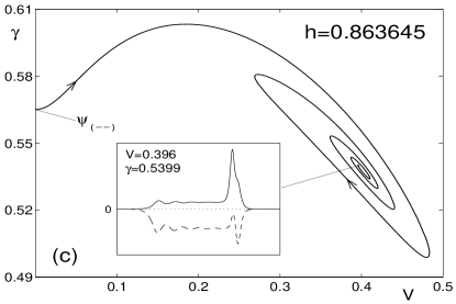
Figure 2: Bifurcation curves branching off the points marked by black dots in Fig.1. The curves illustrate the relation between the value of the damping $\gamma$ and velocity $V$ at which the wave may travel for that $\gamma$. Each curve begins at the point $\gamma=0.565$ on the vertical axis. The insets show representative solutions at internal points of each branch. (Solid line: real part; dashed line: imaginary part.) Note the logarithmic scale of $V$ in (b). Here, and in all other diagrams, arrows indicate our direction of continuation.

The point ‘1’ in Fig.1 corresponds to the stationary complex $\psi_{(++)}$ and lies just above the turning point where the $\psi_{(++)}$ turns into $\psi_{(--)}$. (The turning point has $h=0.83504217$ while $I(h)=0$ for $h=0.8353$.) This solution has four positive real eigenvalues in the spectrum of the associated linearized operator and hence is unstable. The $\gamma(V)$ curve which results from the continuation of this solution in $V$, is shown in Fig.2(a). As $V$ grows from zero, the solution looses its even symmetry (see the inset to Fig.2(a)) while the four positive eigenvalues collide, pairwise, and become two complex conjugate pairs with positive real parts. After reaching a maximum velocity of approximately 0.65, the curve turns back toward $V=0$, with $\gamma$ first growing but then also turning toward $\gamma=0$. The solution transforms into a (strongly overlapped) $\psi_{(+-)}$ complex. As $V$ and $\gamma$ tend to their zero values, the separation between the $\psi_{+}$ and $\psi_{-}$ constituent solitons in the complex grows to infinity. The spectrum becomes the union of the eigenvalues of the individual $\psi_{+}$ and $\psi_{-}$ solitons; in particular, it includes a complex-conjugate pair with positive real part, and a positive real eigenvalue. Thus the entire branch shown in Fig.2(a) is unstable.

One more comment that we need to make here, concerns the validity of the continuation scenario presented in Fig.2(a) for other values of $h$. Note that if we chose a smaller value of $\gamma$ in Fig.1, the value of $h$ corresponding to the point ‘1’ would also be smaller. (For example, for $\gamma=0.548$ the integral $I(h)$ vanishes at the point $h=0.82$.) For this smaller $h$ the final product of the continuation turns out to be not a pair of infinitely separated stationary $\psi_{+}$ and $\psi_{-}$ but a totally different complex. This is discussed below in section V; see also Figs.4(c) and 5.

Another branch bifurcates off at the point marked ‘2’ in Fig.1. Here $h=0.867$. The corresponding $\gamma(V)$ diagram is displayed in Fig.2(b). As we move along the branch departing from $V=0$, the original stationary complex $\psi_{(---)}$ transforms into a solution displaying three widely separated peaks in its real part: one corresponding to a strongly overlapping complex $\psi_{(-+-)}$; the next one to the $\psi_{+}$ and the last one to the $\psi_{-}$ soliton. After passing a turning point, the curve is reapproaching, tangentially, the $V=0$-axis. However, having reached $V=2.2\times 10^{-8}$, it suddenly turns back and the velocity starts to grow again. The separation between the solitons decreases and the solution can now be interpreted as a strongly overlapping four-soliton complex $\psi_{(+++-)}$ (shown in the inset to Fig.2(b)). As we continue further, the four constituent solitons regroup into two complexes, $\psi_{(++)}$ and $\psi_{(+-)}$. The distance between the two complexes grows rapidly and, for certain finite $V$ and $\gamma$ (at the endpoint of the curve in Fig.2(b)) becomes infinite. At this point we have two coexisting solutions, $\psi_{(++)}$ and $\psi_{(+-)}$, and so this point corresponds to the point of self-intersection of the curve shown in Fig.2(a). Continuing the two solutions, separately, from the endpoint of the curve in Fig.2(b), we reproduce the diagram of Fig.2(a) for a slightly different value of $h$ (i.e. for $h=0.867$.)

The entire branch shown in Fig.2 (b) is unstable. The start-off stationary solution $\psi_{(---)}$ has three positive real eigenvalues in its spectrum; one of these persists for all $V$ and $\gamma$ while the other two collide and form a complex-conjugate pair with a positive real part.

The branch continuing from the point ‘3’ in Fig.1, for which $h=0.863645$, leads to the least expected solutions. The resulting $\gamma(V)$ curve is shown in Fig.2(c). For points lying on the ‘spiral’ part of the curve, the function $\psi(x)$ is equal to a constant in a relatively large but finite region, and zero outside that region. (See the inset to Fig.2(c).) The constant is $\psi^{(0)}=(A_{-}/\sqrt{2})e^{-i\theta_{-}}$; it defines a stationary spatially uniform solution to eq.(6). (This flat background is unstable with respect to the continuous spectrum perturbations. Figuratively speaking, our pulse solution $\psi(x)$ represents a ‘droplet’ of the unstable phase in the stable one.) On one side (at the rear of the pulse) the zero background is connected to the background $\psi^{(0)}$ by a kink-like interface. In the front of the pulse, the interface has the character of a large-amplitude excitation, with the shape reminding the $\psi_{(+-)}$ complex. As the curve $\gamma(V)$ spirals toward its ‘focus’ in Fig.2(c), the length of the region where $\psi(x)=\psi^{(0)}$ is growing. The entire branch is unstable; the start-off $\psi_{(--)}$ solution already has two real positive eigenvalues in its spectrum and more appear as we move along the branch. Those additional positive eigenvalues are remnants of the ‘unstable’ interval of the continuous spectrum of the flat nonzero solution $\psi^{(0)}$.

IV Continuation of traveling waves to nonzero dampings

IV.1 Continuability conditions

When $\gamma=0$, the equation (8) has a plethora of localized solutions with nonzero $V$ Baer , and our second strategy will be to attempt to continue these undamped traveling waves to nonzero $\gamma$. We start with establishing the necessary and sufficient conditions for such a continuation.

A set of the necessary conditions can be easily derived using two integral characteristics of equation (6), the momentum

$$P=(i/2)\int(\overline{\psi}_{x}\psi-\psi_{x}\overline{\psi})dx,$$ (22)

and energy (11). No matter whether $\gamma$ equals zero or not, the uniformly traveling solitary waves (i.e. solutions of the form (7)) satisfy $\dot{P}=\dot{E}=0$. Using these relations in eqs.(4) and (12) with $\gamma\neq 0$, we get

$$P=0,$$ (23)

and

$$E=\int|\psi|^{4}dx.$$ (24)

Equations (23)-(24) have to be satisfied by the undamped solutions continuable to nonzero $\gamma$.

In fact, eqs.(23) and (24) are not independent. Indeed, multiplying Eq.(8) by $\overline{\psi}$, adding its complex conjugate and integrating, gives an identity

$$E-\int|\psi|^{4}dx=VP.$$ (25)

Letting $P=0$ in (25), eq.(24) immediately follows. Thus we can keep equation $P=0$ as the only necessary condition for the continuability to nonzero $\gamma$; eq.(24) is satisfied as soon as eq.(23) is in place.

It turns out that $P=0$ is also a sufficient condition. To show this, we expand the field $\psi=u+iv$ in powers of $\gamma$:

$$u=u_{0}+\gamma u_{1}+\gamma^{2}u_{2}+...,\quad v=v_{0}+\gamma v_{1}+\gamma^{2}v_{2}+...,$$

substitute into (8) and equate coefficients of like powers. (We could have also expanded $h$ and $V$ in $\gamma$, but, similarly to the continuation in $V$ described in the previous section, the terms with coefficients $h_{1}$ and $V_{1}$ cancel out of the resulting continuability condition.) At the order ${\cal O}(\gamma^{1})$, we obtain:

$${\cal H}_{0}\left(\begin{array}[]{l}u_{1}\\ v_{1}\end{array}\right)=\left(\begin{array}[]{r}-v_{0}\\ u_{0}\end{array}\right).$$ (26)

Here the hermitian operator ${\cal H}_{0}$ is as in (10) where we only need to attach zero subscripts to $u$ and $v$:

$${\cal H}_{0}=\left(\begin{array}[]{lr}-\partial_{\xi}^{2}+1+h-6u_{0}^{2}-2v_{0}^{2}&-V\partial_{\xi}-4u_{0}v_{0}\\ V\partial_{\xi}-4u_{0}v_{0}&-\partial_{\xi}^{2}+1-h-2u_{0}^{2}-6v_{0}^{2}\end{array}\right).$$ (27)

Since the operator ${\cal H}_{0}$ has a zero eigenvalue, with the translation mode as an associated eigenvector, equation (26) is only solvable if its right-hand side is orthogonal to $(u^{\prime}_{0},v^{\prime}_{0})$:

$$\int(u^{\prime}_{0},v^{\prime}_{0})\left(\begin{array}[]{r}-v_{0}\\ u_{0}\end{array}\right)\,d\xi\phantom{=}=0.$$ (28)

(Here the prime indicates the derivative with respect to $\xi$.) The expression in the left-hand side of (28) coincides with equation (22) written in terms of the real and imaginary part of $\psi$, and so the solvability condition (28) is simply $P=0$.

Now assume that $P$ is equal to zero so that a bounded solution to equation (26) exists. All traveling waves found in Baer have even real and odd imaginary parts: $u_{0}(-x)=u_{0}(x)$, $v_{0}(-x)=-v_{0}(x)$. Noticing that the diagonal elements of the operator ${\cal H}_{0}$ are parity-preserving while the off-diagonal elements change their sign under the $\xi\to-\xi$ reflection, we conclude that $u_{1}(x)$ is odd and $v_{1}(x)$ is even.

Proceeding to the order ${\cal O}(\gamma^{2})$, we have

$${\cal H}_{0}\left(\begin{array}[]{l}u_{2}\\ v_{2}\end{array}\right)=\left(\begin{array}[]{r}-v_{1}+u_{0}[6u_{1}^{2}+2v_{1}^{2}]+4v_{0}u_{1}v_{1}\\ u_{1}+v_{0}[2u_{1}^{2}+6v_{1}^{2}]+4u_{0}u_{1}v_{1}\end{array}\right).$$ (29)

The top entry in the right-hand side of (29) is even and the bottom one odd; hence the right-hand side is orthogonal to the null vector $(u_{0}^{\prime},v_{0}^{\prime})$ and a bounded solution $u_{2}(\xi),v_{2}(\xi)$ exists. This time the $u$-component is even and the $v$-component odd: $u_{2}(-\xi)=u_{2}(\xi)$, $v_{2}(-\xi)=-v_{2}(\xi)$.

It is not difficult to verify that this parity alternation property guarantees the boundedness of $u_{n}(\xi)$ and $v_{n}(\xi)$ for all $n$. Therefore, equation (8) has a localized solution ($\psi(\xi)\to 0$ as $|\xi|\to\infty$) for sufficiently small $\gamma$. Thus if we have an undamped soliton traveling with zero momentum, it can be continued to nonzero values of $\gamma$.

IV.2 Continuable solutions: the bifurcation diagram of the undamped nonlinear Schrödinger

In this subsection we review the $P(V)$ dependence for the undamped solitons and solitonic complexes Baer . Of interest, of course, are points where the graph crosses the $V$-axis, i.e. where $P(V)=0$.

The simplest solutions arising for $V=0$ are, obviously, our stationary fundamental solitons $\psi_{+}$ and $\psi_{-}$. These are given by eqs.(13) where one only needs to set $\gamma=0$:

$$\psi_{+}(x)=A_{+}{\rm sech}\,(A_{+}x),\quad\psi_{-}(x)=iA_{-}{\rm sech}\,(A_{-}x),$$

with $A^{2}_{\pm}=1\pm h$. Both $\psi_{+}$ and $\psi_{-}$ have zero momenta and therefore, are continuable to nonzero $\gamma$. However, the continuation does not produce any traveling waves in this case; all we get is our static damped solitons $\psi_{\pm}$, eq.(13).

Next, both $\psi_{+}$ and $\psi_{-}$ admit continuation to nonzero $V$ (for the fixed $\gamma=0$) Baer . As $V$ is increased to

$$c=\sqrt{2+2\sqrt{1-h^{2}}},$$

the width of the soliton $\psi_{-}$ increases, its amplitude decreases and the soliton gradually transforms into the trivial solution, $\psi\equiv 0$. On the resulting branch, the momentum vanishes only for $V=0$ and $V=c$ and therefore, no damped branches can bifurcate off the traveling $\psi_{-}$ soliton.

We now turn to the soliton $\psi_{+}$. When $h<0.28$, its fate is similar to that of the $\psi_{-}$: as $V\rightarrow c$, the soliton spreads out and merges with the zero solution. The momentum equals zero only at two points, $V=0$ and $V=c$; for $0<V<c$, the momentum is positive.

For $h>0.28$, the transformation of the $\psi_{+}$ is more promising from the present viewpoint (see the dashed curve in Fig.3). As $V$ is increased from zero, the momentum grows, then the branch turns back toward the $V=0$ axis. For some $V<0$ the momentum reaches its maximum and then decreases to zero. The point $V=V_{1}$ where $P(V_{1})=0$ is of interest to us as a branch of damped solitons can bifurcate off at this point (and it really does, see subsection IV.4.) Continuing beyond $V_{1}$, the curve $P(V)$ turns toward $V=0$ and then, after one more turning point, we have another zero crossing: $P(V_{2})=0$. This is how far we have managed to advance in our previous work Baer .

At this point we need to mention that the $\psi_{+}$ and $\psi_{-}$ are not the only quiescent solitons for $\gamma=0$. The dashed $P(V)$ curve in Fig.3 is seen to have one more intersection with the $P$ axis, apart from the one at the origin. The corresponding solution represents a symmetric strongly overlapping complex of the $\psi_{+}$ and $\psi_{-}$ solitons and was coined “twist” (symbolically $\psi_{T}$) in Baer . The twist soliton arises both for $h$ greater and smaller than $0.28$. In the former region the twist obtains from the $V$-continuation of the $\psi_{+}$ soliton while for $h<0.28$, it is not connected to the $\psi_{+}$. (See the solid curve in Fig.3.) The continuation of the twist in $V$ in the case $h<0.28$ gives rise to a new branch of the undamped solutions which has a point of intersection with the $P=0$ axis, at some $V=V_{1}$. A damped traveling wave is bifurcating off at this value of velocity; see the next subsection. We are using the same notation $V_{1}$ in the small- and large-$h$ case in Fig.3 to emphasize the similarity of the resulting $\gamma(V)$ curves in the two cases (forthcoming).

Returning to the case of large $h$, the entire dashed curve in Fig.3 corresponds to symmetric solutions: $\psi(-\xi)={\overline{\psi}}(\xi)$. It turns out that there are also non-symmetric solutions; these were missed in Baer . The real part of a non-symmetric solution is not even and imaginary part not odd. In particular, a pair of asymmetric solutions arise in a pitchfork bifurcation of the complex $\psi_{(TT)}$; see the dash-dotted offshoot from the dashed curve in Fig.3. (The two asymmetric solutions are related by the transformation $\psi(\xi)\to{\overline{\psi}}(-\xi)$; they obviously have equal momenta and hence are represented by the same curve.) Continuing the asymmetric branch we have the third zero crossing, at $V=V_{3}$. When continued to positive $P$, the asymmetric solution acquires the form of a complex of $\psi_{-}$ and $\psi_{T}$ solitons, with the inter-soliton separation growing as $P$ is increased. (Note that although the dashed and dash-dotted curve end at nearby points, they are not connected.) Our numerical analysis shows that branches of damped solitons do indeed detach at $V_{1}$, $V_{2}$ and $V_{3}$; these will be described in the next two subsections.

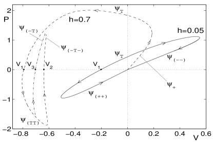
Figure 3: The momentum of the undamped traveling wave as a function of its velocity (a combined and advanced version of two diagrams from Baer ). The dashed and dash-dotted curves pertain to the case of large driving strengths (here exemplified by $h=0.7$). The starting point $P=V=0$ of the dashed curve corresponds to the stationary undamped $\psi_{+}$ soliton, which then transforms to the twist, then to a bound state of two twists and then to a complex of a twist and two $\psi_{-}$ solitons. (This curve appeared in Baer .) The dash-dotted offshoot is our new contribution to the diagram; it corresponds to an asymmetric solution, $\psi_{(-T)}$, detaching from the $\psi_{(TT)}$ curve. The solid curve pertains to the case of small driving amplitudes (here $h=0.05$). (This curve also appeared in Baer .) The points of its intersection with the $P$-axis correspond to stationary twist solitons; continuing each of these counterclockwise gives rise to a bound state of two $\psi_{+}$’s, while when continued clockwise each twist transforms into a complex of two $\psi_{-}$’s. More solution curves can be generated by the mapping $V\to-V$, $P\to-P$.

IV.3 Numerical continuation: Small driving amplitudes

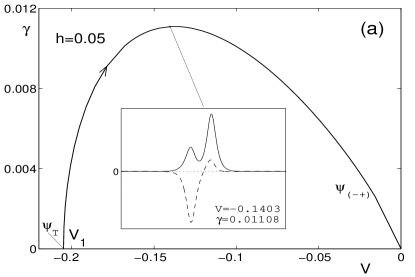
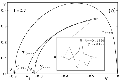
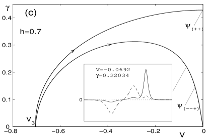
Figure 4: Results of the numerical continuation of the undamped traveling solitons to nonzero $\gamma$. (a): small $h$; (b),(c): large $h$. The inset displays a representative solution at one of the internal points of the curve. (Solid line: real part; dashed line: imaginary part.) Each curve shown has a positive-velocity counterpart which arises by the mirror reflection $V\to-V$ of the figure.

For small $h$, $h<0.28$, our continuation departs from the twist soliton moving with the velocity $V_{1}$ (the point of intersection of the solid curve with the horizontal axis in Fig.3.) The real part of this solution is even and imaginary part odd: $\psi(-x)={\overline{\psi}}(x)$. As we continue to nonzero $\gamma$, this symmetry is lost; a typical profile at the internal points looks like a non-symmetric complex of the $\psi_{-}$ and $\psi_{+}$ and is displayed in the inset to Fig.4(a). The rest of Fig.4(a) shows the resulting $\gamma(V)$ dependence. As $\gamma$ grows, the negative velocity of the traveling wave decreases in modulus. However the damping cannot be increased beyond a certain limit value; as we reach it, the $\gamma(V)$-curve turns down (Fig.4(a)). As $V$ and $\gamma$ tend to zero, the separation between the $\psi_{-}$ and $\psi_{+}$ solitons in the complex grows without bounds.

These transformations of the solution are reflected by the behavior of the linearized eigenvalues in the eigenvalue problem (9). At the point $V=V_{1}$, $\gamma=0$ of the $\gamma(V)$ curve, the twist solution has a quadruplet of complex eigenvalues $\pm\lambda,\pm{\overline{\lambda}}$ which dissociates into two pairs of complex-conjugate eigenvalues $\lambda_{1},{\overline{\lambda}_{1}}$ and $\lambda_{2},{\overline{\lambda}_{2}}$ (with ${\rm Re}\,\lambda_{1}<0$ and ${\rm Re}\,\lambda_{2}>0$) as $\gamma$ deviates from zero. As we move toward the maximum of the curve, the imaginary parts of $\lambda_{1}$ and $\lambda_{2}$ decrease and the four complex eigenvalues move onto the real axis. At the point of maximum one of the resulting two positive eigenvalues crosses to the negative real axis, but the other one persists all the way to $V=-0$ and $\gamma=+0$. Therefore the spectrum of eigenvalues on the ‘downhill’ portion of the curve is a union of eigenvalues of the $\psi_{-}$ and $\psi_{+}$ solitons. The conclusion of the eigenvalue analysis is that the traveling complex whose bifurcation diagram is exhibited in Fig.4(a), is unstable for all $V$ and $\gamma$.

IV.4 Numerical continuation: Large driving amplitudes

For $h>0.28$ we have three starting points with $P=0$ corresponding to two intersections of the dashed curve and one of the dash-dotted curve with the horizontal axis in Fig.3.

The $\gamma(V)$ curve emanating out of the point $V_{1}$ is the top, arc-shaped, curve in Fig.4(b). For $V=V_{1}$ and $\gamma=0$ the solution is symmetric and its shape reminds two strongly overlapping twists. The linearized spectrum includes two complex quadruplets. As $\gamma$ deviates from zero, the symmetry is lost and the solution starts looking like an asymmetric complex of two pulses. The two complex quadruplets become four complex-conjugate pairs of eigenvalues, two with positive and two with negative real parts. Two of these pairs (one with $\mbox{Re}\,\lambda>0$ and one with $\mbox{Re}\,\lambda<0$) move on to the real axis. After that one positive real eigenvalue crosses to the negative semi-axis, while the complex pair with $\mbox{Re}\,\lambda>0$ crosses into the $\mbox{Re}\,\lambda<0$ half-plane but then returns to $\mbox{Re}\,\lambda>0$. As $V,\gamma\to 0$, the separation between the $\psi_{-}$ and $\psi_{+}$ solitons comprising this complex increases, and eventually the two constituents diverge to infinities. On the ‘downhill’ portion of the curve, the spectrum is a union of the spectra of the individual $\psi_{-}$ and $\psi_{+}$ solitons; in particular, it includes a positive real eigenvalue and a complex quadruplet. Since there are eigenvalues with ${\rm Re}\,\lambda>0$ for all $V$, the entire branch is unstable.

The second undamped traveling wave with zero momentum (point $V_{2}$ on the bifurcation diagram Fig.3) corresponds to a symmetric [$\psi(-x)={\overline{\psi}}(x)$] complex of two $\psi_{-}$ and one twist soliton, symbolically $\psi_{(-T-)}$. The spectrum includes three complex quadruplets. As we continue in $\gamma$ and $V$, the symmetry is lost but the solution still looks like a complex of three solitons, see the inset to Fig.4(b). The bottom, spike-shaped, curve in Fig.4(b) depicts the corresponding $\gamma(V)$ dependence. Unlike the branch starting at the value $V=V_{1}$, this solution cannot be continued to zero velocities. Instead, the $\gamma(V)$ curve turns back and, as $\gamma$ approaches zero from above, $V$ tends to a negative value $V_{4}$, with $|V_{4}|>|V_{2}|$. For sufficiently small $\gamma$ the corresponding solution consists of two $\psi_{-}$ solitons and a twist in between, with the inter soliton separations growing to infinity as $\gamma\to 0$, $V\to V_{4}$. The associated eigenvalues perform rather complicated movements on the complex plane; skipping the details it suffices to mention that ‘unstable’ eigenvalues (real positive or complex with positive real parts) are present for all $V$. Hence the entire branch is unstable.

Finally, the point $V_{3}$ on the diagram Fig.3 represents two nonequivalent asymmetric solutions with zero momentum, $\psi_{1}(\xi)$ and $\psi_{2}(\xi)$, with $\psi_{2}(\xi)\equiv{\overline{\psi}_{1}}(-\xi)$. Consequently, there are two distinct $\gamma(V)$-branches coming out of this point (Fig.4(c)). One of these corresponds to a complex of two solitons; when continued to $V=0$, it gives rise to the symmetric complex $\psi_{(++)}$ with nonzero $\gamma$. (See the top curve in Fig.4(c)). Continuing the other asymmetric solution to $V=0$, the corresponding value of $\gamma$ reaches a maximum at $V\sim 0.3$ and then tends to zero. (The bottom curve in Fig.4(c)). For sufficiently small $V$ and $\gamma$ this solution represents a complex $\psi_{(--+)}$ (shown in the inset to Fig.4(c)). As $V,\gamma\to 0$, the inter-soliton separation tends to infinity. Turning to the eigenvalues, the start-off solution at the point $V_{3}$ has two complex quadruplets and a real positive eigenvalue in its spectrum. When we continue along the top curve in Fig.4(c), two complex eigenvalues move on to the positive real axis, so we end up with three positive eigenvalues. When we continue along the bottom curve, the movements of the eigenvalues are more involved but some of them always remain in the ‘unstable’ half-plane, ${\rm Re}\,\lambda>0$. The upshot of the eigenvalue analysis is that both curves represent only unstable solutions.

V Consistency of the two approaches

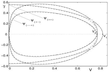
Figure 5: The comparison of the bifurcation diagrams for $h=0.82$ and $h=0.8275$. Solid curve: $h=0.8275$; dashed curve: $h=0.82$. Although the points of intersection of the dashed and solid curves with the $V$-axis do not coincide, i.e. $V_{3}(0.8275)\neq V_{3}(0.82)$ and $V_{1}(0.8275)\neq V_{1}(0.82)$, they are quite close to each other and hence we mark them as a single point ($V_{3}$ and $V_{1}$, respectively.) The branches coming out of the point $V_{2}$ on the $V$-axis are omitted for visual clarity. Note the shape of the dashed and solid curves near $V\sim 0.7$, $\gamma\sim 0.3$, characteristic of phase portraits of 2D dynamical systems in the neighborhood of saddle points.

To complete our classification of damped traveling solitons, we need to comment on what may seem to be an inconsistency between results obtained within the above two complementary approaches. The solution representing the well-separated $\psi_{+}$ and $\psi_{-}$ solitons reported in sections III and IV, can be reached by continuing both off the $(\gamma=0)$- and $(V=0)$-axes. (This branch connecting to the origin on the $(V,\gamma)$-plane appears both in Figs. 2(a) and 4(b).) Although such a curve should obviously not depend on the starting point of the continuation, one notices that the $\psi_{(+-)}$ branches ‘flowing into the origin’ in Figs. 2(a) and 4(b) behave differently when traced backward (i.e. away from $V=\gamma=0$). While the curve in Fig.2(a) intersects the $\gamma$-axis, its counterpart in Fig.4(b) crosses the other, $V$-, axis. (Here the reader should not be confused by the fact that the $\psi_{(+-)}$ branch in Fig.2(a) is shown for positive and its counterpart in Fig.4(b) for negative values of $V$. In view of the $\xi\to-\xi$, $V\to-V$ invariance of equation (8), to each $\gamma$ there correspond two traveling waves, one with positive and the other one with negative value of $V$. Therefore, one should mirror-reflect Fig.4(b) prior to comparing it to Fig.2(a). This reflection maps the solution $\psi_{(-+)}$ of Fig.4(b) to the $\psi_{(+-)}$ of Fig.2(a).)

To resolve the paradox, one needs to note that the two figures correspond to different values of $h$, Fig.2(a) to $h=0.8353$ and Fig.4(b) to $h=0.7$. It turns out that a qualitative change of behavior occurs for $h$ somewhere between these values, more precisely between $0.82$ and $0.8275$: For $h=0.82$ and smaller (in particular, for $h=0.7$) the $\gamma(V)$ curve has the form of an arc shown in Fig.4(b) (i.e. it crosses the $V$-axis as $V$ is increased) while for $h=0.8275$ and greater, the curve is already loop-shaped and does not reach to $\gamma=0$. This change of behavior, accounting for the above ‘inconsistency’, is illustrated by Fig.5 which compares the $\gamma(V)$ dependences for $h=0.82$ and $h=0.8275$. Fig.5 also serves to illustrate the different outcomes of the continuation of the complex $\psi_{(++)}$ for $h=0.8353$ and smaller $h$. (We note that for $h=0.8353$ the continuation of the motionless $\psi_{(++)}$ produces a pair of infinitely separated solitons $\psi_{+}$ and $\psi_{-}$ [Fig.2(a)] while for $h=0.7$, the curve departing from the same type of starting point [i.e. from $\psi_{(++)}$] ends up at the undamped asymmetric solution traveling with nonzero velocity $V_{3}$ [Fig.4(c)].)

The above differences in behavior result from the presence of a saddle point on the $(\gamma,V)$-plane, in the gap between the two lobes of the solid curve in Fig.5. Indeed, the dashed and solid curves can be seen as sections of the surface $h=h(\gamma,V)$ by the horizontal planes $h=0.82$ and $h=0.8275$, respectively. The gap in the upper solid curve is then accounted for by letting $h=h_{0}+x^{2}-y^{2}$ in the vicinity of the gap. Here the constant $h_{0}$ lies somewhere between $0.82$ and $0.8275$, and $(x,y)$ is a pair of suitably chosen coordinates on the $(\gamma,V)$-plane.

VI Conclusions

One of the conclusions of this work is that by grouping into complexes, solitons (or, equivalently, solitary pulses) can adjust their total momentum to zero. By doing so they can travel with nonzero speed in the presence of damping — without violating the momentum decay law, ${\dot{P}}=-\gamma P$. Two identical solitons traveling at the same speed in the same direction have equal momenta; therefore, in order to arrange for $P=0$ the traveling complex inevitably has to include solitons of different varieties (i.e. both $\psi_{+}$’s and $\psi_{-}$’s.) Consequently, the real and imaginary parts of the traveling complex will always be represented by asymmetric functions of $\xi=x-Vt$.

Although the possibility of non-decelerated motion may be out of line with the common perception of the soliton dynamics in weakly damped Hamiltonian equations, moving pulses are not unknown in strongly dissipative systems. A suitable example is given by the complex Ginzburg-Landau equation. Asymmetric Ginzburg-Landau pulses, uniformly traveling with nonzero velocities, were reported in Afanasjev .

All moving solutions that we have found in this paper, turned out to be unstable. This instability admits a simple qualitative explanation — at least, for small dampings. In the undamped situation, the $\psi_{-}$ solitons are unstable when traveling with small velocities while the $\psi_{+}$’s become unstable when moving sufficiently fast Baer . In the presence of dissipation the traveling wave has to include solitons of both varieties; on the other hand, the eigenvalues corresponding to small nonzero $\gamma$ should remain close to their ($\gamma=0$)-counterparts. Therefore the spectrum of the traveling complex will ‘inherit’ unstable eigenvalues of either $\psi_{-}$ (for small velocities) or of the $\psi_{+}$ (for large velocities).

Thus, despite the fact that the parametric driver can sustain the uniform motion of a damped soliton, an additional agent (such as, possibly, the diffusion and/or a nonlinear damping term) is required to make this motion stable. Here it is appropriate to refer, again, to the complex Ginzburg-Landau equation. Stable Ginzburg-Landau pulses arise as a result of a delicate balance of the whole series of terms, including dispersion, cubic and quintic nonlinearity, diffusion, cubic gain and linear and quintic nonlinear damping stableGL ; Afanasjev ; Akhmediev . In a similar way, the gain/loss and spreading/steepening balances of the damped-driven traveling solitons could be restored by adding one or several missing agents.

- (1) Email address: igor@cenerentola.mth.uct.ac.za; igor@maths.uct.ac.za
- (2) Permanent address: Laboratory for Information Technologies, Joint Institute for Nuclear Research, Dubna 141980, Russia. Email address: elena@jinr.ru
- (3) J.W. Miles, J. Fluid Mech. 148, 451 (1984)
- (4) C. Elphick and E. Meron, Phys. Rev. A 40, 3226 (1989)
- (5) X.N. Chen and R.J. Wei, J. Fluid Mech. 259, 291 (1994); W. Zhang and J. Viñals, Phys. Rev. Lett. 74, 690 (1995); W. Wang, X. Wang, J. Wang, and R. Wei, Phys. Lett. A 219, 74 (1996); X. Wang and R. Wei, Phys. Rev. Lett. 78, 2744 (1997); Phys. Rev. E 57, 2405 (1998); A. Il’ichev, Physica D 119, 327 (1998); G. Miao and R. Wei, Phys. Rev. E 59, 4075 (1999); D. Astruc and S. Fauve. Parametrically Amplified 2-Dimensional Solitary Waves. In: IUTAM Symposium on Free Surface Flows. Proceedings of the IUTAM Symposium held in Birmingham, UK, 10-14 July 2000. A. C. King and Y. D. Shikhmurzaev, editors. Fluid Mechanics and Its Applications, Vol. 62 (Kluwer, 2001).
- (6) I.H. Deutsch and I. Abram, J. Opt. Soc. Am. B11, 2303 (1994); A. Mecozzi, L. Kath, P. Kumar, and C.G. Goedde, Opt. Lett. 19, 2050 (1994); S. Longhi, Opt. Lett. 20, 695 (1995); Phys. Rev. E 55, 1060 (1997); V.J. Sánchez-Morcillo, I. Pérez-Arjona, F. Silva, G.J. de Valcárcel, and E. Roldán, Opt. Lett. 25, 957 (2000)
- (7) I.V. Barashenkov, M.M. Bogdan, and V.I. Korobov, Europhys. Lett. 15, 113 (1991)
- (8) B. Denardo, B. Galvin, A. Greenfield, A. Larraza, S. Putterman, and W. Wright, Phys. Rev. Lett. 68, 1731 (1992); W.-Z. Chen, Phys. Rev. B49, 15063 (1994); G. Huang, S.-Y. Lou, and M. Velarde, Int. J. of Bifurcation and Chaos, 6, 1775 (1996); N.V. Alexeeva, I.V. Barashenkov, and G.P. Tsironis, Phys. Rev. Lett. 84, 3053 (2000); W. Chen, B. Hu, H. Zhang, Phys. Rev. B 65, 134302 (2002)
- (9) D.J. Kaup and A.C. Newell, Proc. R. Soc. Lond. A 361, 413 (1978)
- (10) I.V. Barashenkov and Yu.S. Smirnov, Phys. Rev. E 54, 5707 (1996)
- (11) G. Terrones, D.W. McLaughlin, E.A. Overman, A. Pearlstein, SIAM J. Appl. Math. 50, 791 (1990); I.V. Barashenkov and E.V. Zemlyanaya, Physica D 132, 363 (1999)
- (12) B.A. Malomed, Phys. Rev. A 44, 6954 (1991); D. Cai, A.R. Bishop, N. Grønbech-Jensen, and B.A. Malomed, Phys. Rev. E 49, 1677 (1994)
- (13) I.V. Barashenkov, Yu.S. Smirnov, and N.V. Alexeeva, Phys. Rev. E 57, 2350 (1998); M. Kollmann, H.W. Capel, and T. Bountis, Phys. Rev. E 60, 1195 (1999);
- (14) I.V. Barashenkov and E.V. Zemlyanaya, Phys. Rev. Lett. 83, 2568 (1999)
- (15) D.J. Kaup and A.C. Newell, Phys. Rev. B 18, 5162 (1978)
- (16) C. Elphick and E. Meron, Phys. Rev. Lett. 65, 2476 (1990)
- (17) Yu.S. Kivshar and B.A. Malomed, Rev. Mod. Phys. 61, 763 (1989)
- (18) V.S. Shchesnovich and I.V. Barashenkov, Physica D 164, 83 (2002)
- (19) I.V. Barashenkov, E.V. Zemlyanaya, and M. Bär. Phys. Rev. E 64, 016603 (2001)
- (20) P. Coullet, J. Lega, B. Houchmanzadeh, and J. Lajzerowicz, Phys. Rev. Lett. 63, 1352 (1990); P. Coullet, J. Lega, and Y. Pomeau, Europhys. Lett. 15, 221 (1991); P. Coullet and K. Emilsson, Physica D 61, 119 (1992); B.A. Malomed and A.A. Nepomnyashchy, Europhys. Lett. 27, 649 (1994); C. Elphick, A. Hagberg, B.A. Malomed, and E. Meron, Phys. Lett. A 230, 33 (1997); S. Longhi, Phys. Rev. E 55, 1060 (1997); D.V. Skryabin, A. Yulin, D. Michaelis, W.J. Firth, G.-L. Oppo, U. Peschel, and F. Lederer, Phys. Rev. E 64, 056618 (2001); C. Utzny, W. Zimmermann, and M. Bär, Europhys. Lett. 57, 113 (2002); G.J. de Valcárcel, I. Pérez-Arjona, and E. Roldán, Phys. Rev. Lett. 89, 164101 (2002)
- (21) V.V. Afanasjev, N. Akhmediev and J.M. Soto-Crespo, Phys. Rev. E 53, 1931 (1996)
- (22) O. Thual and S. Fauve, J. Phys. (Paris) 49, 1829 (1988); S. Fauve and O. Thual, Phys. Rev. Lett. 64, 282 (1990)
- (23) N. Akhmediev and A. Ankiewicz. Solitons of the Complex Ginzburg-Landau Equation. In: S. Trillo, W. Torruellas (Eds.) Spatial Solitons. Springer Series in Optical Sciences, vol. 82, 2001