Stochastic resonance between noise-sustained patterns

Abstract

We study an extended system that without noise shows a spatially homogeneous state, but when submitted to an adequate multiplicative noise, some noise-induced patterns arise. The stochastic resonance between these structures is investigated theoretically in terms of a two-state approximation. The knowledge of the exact nonequilibrium potential allows us to obtain the output signal-to-noise ratio. Its maximum is predicted in the symmetric case for which both stable attractors have the same nonequilibrium potential value.

I Introduction

During the last few decades a wealth of research results on fluctuations or noise have lead us to the recognition that in many situations noise can actually play a constructive role that induces new ordering phenomena. Some examples are stochastic resonance in zero-dimensional and extended systems RMP ; extend1 ; extend2 ; extend2b ; extend3a ; extend3b , noise-induced transitions lefev , noise-induced phase transitions nipt1 ; nipt2 , noise-induced transport Ratch2 ; Ratch3 ; nipt3 ; nipt4 , noise-sustained patterns ga93 ; nsp ; ber , noise-induced limit cycle mangwio , etc.

The phenomenon of stochastic resonance (SR)— namely, the enhancement of the output signal-to-noise ratio (SNR) caused by injection of an optimal amount of noise into a nonlinear system— stands as a puzzling and promising cooperative effect arising from the interplay between deterministic and random dynamics in a nonlinear system. The broad range of phenomena— drawn from almost every field in scientific endeavor— for which this mechanism can offer an explanation has been put in evidence by many reviews and conference proceedings. See Ref.RMP and references there to scan the state of the art.

Most of the phenomena that could possibly be explained by SR occur in extended systems: for example, diverse experiments were carried out to explore the role of SR in sensory and other biological functions biol or in chemical systems sch . These were, together with the possible technological applications, the motivation to many recent studies showing the possibility of achieving an enhancement of the system response by means of the coupling of several units in what conforms an extended medium extend1 ; otros ; extend2 ; extend3a ; extend3b , or analyzing the possibility of making the system response less dependent on a fine tuning of the noise intensity, as well as different ways to control the phenomenon claudio ; nos3 .

In some previous papers extend2 ; extend2b ; extend3a ; extend3b we have studied the stochastic resonant phenomenon in extended systems for the transition between two different patterns, and exploiting the concept of nonequilibrium potential GR ; I0 . The nonequilibrium potential is a special Lyapunov functional of the associated deterministic system which for nonequilibrium systems plays a role similar to that played by a thermodynamic potential in equilibrium thermodynamics GR . Such a nonequilibrium potential, closely related to the solution of the time independent Fokker-Planck equation of the system, characterizes the global properties of the dynamics: that is attractors, relative (or nonlinear) stability of these attractors, height of the barriers separating attraction basins, and in addition it allows us to evaluate the transition rates among the different attractors.

In this work we analyze a new aspect of such a problem studying SR between two noise-induced-patterns ga93 ; nsp , that is: the same noise source that induces and supports the existence of the patterns is the one that induces the transitions among them, and produces the stochastic resonant phenomenon. Some related work correspond to the misleadingly called double stochastic resonance ZKSG , as well as to another previous work MGOC related with noise-induced phase transitions nipt1 ; nipt2 . In both cases the authors have only resorted to a standard mean-field approach, while here we obtain the exact form of the noise-induced patterns (stable and unstable ones) as well as the complete form of the nonequilibrium potential. In this way we can obtain the transition rates and clearly quantify the SR phenomenon by means of the SNR.

The organization of the paper is as follows. In section II we present the model and formalism to be used. After that, we discuss in section III the stochastic resonance between the noise-sustained structures. Finally, we present in section IV some conclusions and future perspectives.

II The Model

We consider a one-dimensional system described by the following deterministic equation

$$\partial_{t}\phi(x,t)=\partial_{x}(D(\phi)\partial_{x}\phi)+F(\phi),$$ (1)

that can be written in a variational form as

$$\partial_{t}\phi(x,t)=-\frac{1}{D(\phi)}\frac{\delta V[\phi]}{\delta\phi(x)},$$ (2)

where the potential

$$V[\phi]=\int_{-L/2}^{L/2}dx\bigg{\{}-\int_{0}^{\phi}d\phi^{\prime}D(\phi^{\prime})F(\phi^{\prime})+\frac{1}{2}\big{[}D(\phi)\partial_{x}\phi\big{]}^{2}\bigg{\}}$$ (3)

is a Lyapunov functional (while $D(\phi)>0$) for the deterministic dynamics and it is essentially the logarithm of the probability density of configuration when Eq.(1) is perturbed by an additive source of spatiotemporal white noise.

The starting point of our stochastic analysis will be Eq. (1) with an additional multiplicative noise, in the Stratonovich interpretation, given by

$$\partial_{t}\phi(x,t)=-\frac{1}{D(\phi)}\frac{\delta V[\phi]}{\delta\phi(x)}+g(\phi)\xi(x,t),$$ (4)

where $\xi$ is a Gaussian noise with zero mean and correlation $\langle\xi(x,t)\xi(x^{\prime},t^{\prime})\rangle=2\epsilon^{2}\delta(x-x^{\prime})\delta(t-t^{\prime})$, being $\epsilon^{2}$ the noise intensity. For the coefficient of the noise term, $g(\phi)$, we adopt

$$g(\phi)=\frac{1}{\sqrt{D(\phi)}},$$ (5)

in order to guarantee that the fluctuation-dissipation relation is fulfilled kitara .

As we are considering the Stratonovich interpretation, the stationary solution of the associated Fokker-Planck equation can be written as ibanyes

$$P_{st}[\phi]\sim\exp(-V_{eff}/\epsilon^{2}),$$ (6)

where the effective potential $V_{eff}[\phi]$ is given by

$$V_{eff}[\phi]=V[\phi]-\lambda\int_{-L/2}^{L/2}dx\ln D(\phi).$$ (7)

Here $\lambda$ is a renormalized parameter related to $\epsilon$ through $\lambda=\epsilon^{2}/(2\Delta x)$ in a lattice discretization, where $\Delta x$ is the lattice parameter ibanyes .

The extremes of $V_{eff}$ correspond to the (stationary) noise-sustained structures $\phi_{st}$. They can be computed from the first variation of $V_{eff}(\phi)$ respect to $\phi$ equal to zero, that is

$$\delta V_{eff}[\phi_{st}]=-\int_{-L/2}^{L/2}D(\phi)[\partial_{x}(D(\phi)\partial_{x}\phi)+F_{eff}(\phi)]\delta\phi(x)\,dx\bigg{|}_{\phi=\phi_{st}}=0,$$ (8)

where

$$F_{eff}(\phi)=F(\phi)+\lambda\frac{1}{D(\phi)^{2}}\frac{d}{d\phi}D(\phi)$$ (9)

is the effective nonlinearity which drives the dynamics of the noise sustained patterns.

We will consider a finite system, i.e. limited to the region $-L/2\leq x\leq L/2$; and assume Dirichlet boundary conditions, that is $\phi(\pm L/2)=0$. In addition, we consider the case of a monostable dynamics in absence of noise

$$F=-\phi^{3}+b\phi^{2},$$ (10)

and we adopt a model of field-dependent diffusivity which induces an effective bistable dynamics. In particular we have chosen

$$D(\phi)=\frac{D_{0}}{1+h\phi^{2}},$$ (11)

($D_{0},\,h>0$), that corresponds to have a larger diffusivity in low density (low $\phi$) regions and a lower diffusivity in high density (large $\phi$) ones. With this functional form, $F_{eff}(\phi)$ in Eq. (9) results

$$F_{eff}=-\phi^{3}+b\phi^{2}-\frac{2\lambda h\phi}{D_{0}}=\phi(\phi-\phi_{1})(\phi_{2}-\phi),$$ (12)

where $\phi_{1,2}$ depend on parameters, in particular on the control parameter $\lambda$. It is worth noting here that in the deterministic problem ($\lambda=0$) the reaction term is monostable while, as we increase the noise intensity, the effective nonlinear term $F_{eff}$ becomes bistable (within the interval $0<\lambda<b^{2}D_{0}/(8h)$) and finally, for $\lambda>b^{2}D_{0}/(8h)$ becomes again monostable (reentrance effect). Our choice of $F$ and $D$ is one among a plenty of different forms for the diffusivity leading to a transition from monostable to bistable and inducing the SR phenomenon (see for instance the one used in ibanyes , that corresponds exactly to the inverse of the present diffusion coefficient, i.e. $D(\phi)=D_{0}(1+h\phi^{2})$). Density-dependent diffusivities arise in a large variety of systems modeled by reaction-diffusion equations ddd0 . In biology, for instance, population dynamics is usually driven by a diffusivity that depends on the local population ddd1 . We can also find examples in physics, a couple of them are in polymer physics (where the diffusion can abruptly drop several orders of magnitude at the gelation point ddd2 ) and in diffusion of hydrogen in metals ddd3 .

A remarkable point is that $\phi=0$ is always a root of $F_{eff}=0$ (see Fig. 1). This implies (from Eq. (8)) that $\phi(x)\equiv 0$ is an extremum of $V_{eff}[\phi]$ for all values of $\lambda$. In what follows we will call this pattern $\phi_{0}$.

Figure 1: Form of the nonlinearities for the deterministic case ($\lambda=0$), bistable case ($\lambda=0.8$) and a monostable case ($\lambda=1.2$) in the reentrance region. The vertical scale was changed in the deterministic case in order to clarify the figure. The parameters used are: $D_{0}=1$, $h=1/2$ and $b=2$. Note that $\phi=0$ remains as a root in all cases.

In order to obtain the non uniform extremes of the potential (and also of the density probability) we must (numerically) solve

$$\frac{d}{dx}\bigg{(}D(\phi_{st})\frac{d}{dx}\phi_{st}\bigg{)}+F_{eff}(\phi_{st})=0,$$ (13)

for the stationary regimen profiles $\phi_{st}(x)$. This approach allows us to found both, the stable and unstable solutions. To analyze their stability we need to calculate $\delta^{2}V_{eff}$, that defines a Sturm-Liouville problem, with orthogonality weight $D(\phi_{st})$. From that analysis it results that $\phi_{0}$ (defined before) is stable for $\lambda>0$, and in the bistability region we have two nonhomogeneous symmetric patterns: one unstable $\phi_{u}$ (saddle) and one stable $\phi_{s}$. The typical form of these patterns is illustrated in Fig. 2.

Figure 2: Noise-sustained stationary patterns of the problem. We show $\phi_{0}\equiv 0$, the stable homogeneous pattern; and both nonhomogeneous patterns: the unstable (saddle) $\phi_{u}$ and the stable one $\phi_{s}$. Here we have $\lambda=\lambda_{c}\approx 0.8$, while the other parameters values are the same as in Fig. 1

In Fig. 3 we show $V_{eff}[\phi_{st}]$ vs. $\lambda$, evaluated on the different stationary patterns. We define $\lambda_{c}$ as the value of $\lambda$ at which we have symmetrical stability, i. e. where $V_{eff}[\phi_{0}]=V_{eff}[\phi_{s}]$. From this figure it is apparent that, similarly to previous cases I0 , for increasing values of $\lambda$ both nonhomogeneous solutions (the stable and the unstable one) coalesce and disappear in agreement with the above argument about the reentrance effect.

Figure 3: Nonequilibrium potential $V_{eff}[\phi_{st}]$, as a function of $\lambda$, evaluated on the stationary patterns: curves correspond to stable ($\phi_{s}$), homogeneous ($\phi_{0}$) and unstable ($\phi_{u}$) patterns. The arrow indicate the point where $V_{eff}[\phi_{0}]=V_{eff}[\phi_{s}]$, corresponding to $\lambda=\lambda_{c}\approx 0.8$.

III Stochastic resonance between noise-sustained structures

We are interested in the stochastic resonance phenomena occurring in the above described system. For a window of noise intensity the effective dynamics of the system is bistable, corresponding to a noise-induced nontrivial dynamics. We will resort to the so-called two-state approximation McNam , all details about the procedure and the evaluation of the SNR could be found in extend3a . We consider now that the system is subject, in the adiabatic limit, to a time periodic signal of the form $b=b_{0}+S(t)$ where $S(t)=\Delta b\,\sin(\omega_{0}t)$.

Up to first-order in the amplitude $\Delta b$ (assumed to be small in order to have a sub-threshold periodic input) the transition rates $W_{i}$ take the form

$$W_{1}(t) = \mu_{1}-\alpha_{1}\,\Delta b\,\sin(\omega_{0}\,t),$$

$$W_{2}(t) = \mu_{2}+\alpha_{2}\,\Delta b\,\sin(\omega_{0}\,t),$$ (14)

where the constants $\mu_{1,2}$ and $\alpha_{1,2}$ are obtained from the Kramers-like formula for the transition rate Hanggi

$$W_{\phi_{i}\rightarrow\phi_{j}}=\frac{\lambda_{+}}{2\pi}\,\left[\frac{\det\,V_{eff}[\phi_{i}]}{|\det\,V_{eff}[\phi_{u}]|}\right]^{1/2}\,\exp[-(V_{eff}[\phi_{u}]-V_{eff}[\phi_{i}])/\epsilon^{2}].$$ (15)

Here $\lambda_{+}$ is the unstable eigenvalue of the deterministic flux at the relevant saddle point ($\phi_{u})$ and

$$\mu_{1,2} = W_{1,2}|_{S(t)=0}$$

$$\alpha_{1,2} = \mp\frac{dW_{1,2}}{dS(t)}|_{S(t)=0}.$$ (16)

These results allows us to calculate the autocorrelation function, the power spectrum and finally the SNR. The details of the calculation were shown in Ref. extend3a . For the SNR, and up to the relevant (second) order in the signal amplitude $\Delta b$, we obtain

$$R=\,\frac{\pi}{4\,\mu_{1}\,\mu_{2}}\frac{(\alpha_{2}\,\mu_{1}+\alpha_{1}\,\mu_{2})^{2}}{\mu_{1}+\mu_{2}}=\frac{\pi}{4\epsilon^{2}}\,\frac{\mu_{1}\,\mu_{2}}{\mu_{1}+\mu_{2}}\,\Phi,$$ (17)

where

$$\Phi=\int_{-L/2}^{L/2}dx\,\int_{\phi_{0}}^{\phi_{s}(x)}\,D(\phi^{\prime})\,\phi^{\prime 2}\,d\phi^{\prime},$$ (18)

gives a measure of the spatial coupling strength. In our case $\phi_{0}\equiv 0$ and

$$\Phi=D_{0}\int_{-L/2}^{L/2}dx\,\left\{\frac{\phi_{s}(x)}{h}-\frac{\arctan[\sqrt{h}\,\phi_{s}(x)]}{h^{3/2}}\right\}.$$ (19)

In Fig. 4 we show the SNR as a function of parameter $\lambda$ (which is proportional to $\epsilon^{2}$). The existence of the typical maximum is the characteristic fingerprint of SR. For a window of noise intensity values, the system enhances the output to the input periodic signal. We see that the maximum SNR occurs at the symmetric situation, that is at $\lambda=\lambda_{c}$.

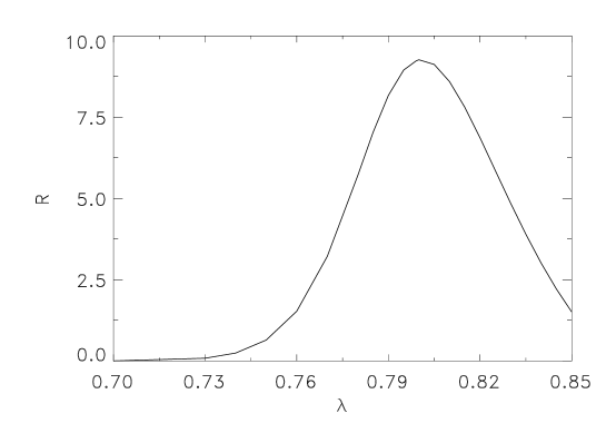
Figure 4: Signal-to-noise ratio vs. $\lambda$. Here $b_{0}=2$, while other parameters remain unchanged.

A similar behavior is observed in general for a wide range of values for $h$ and $D_{0}$ compatible with a bistable effective dynamics. In particular, $\lambda_{c}$ is a monotonically decreasing function of $h$, as we show in Fig. 5. For a given value of $h$, a numerical analysis of Eq. (17) indicates that the maximum of SNR take place at $\lambda_{c}(h)$. Note that, for a given value of $\lambda$, $h$ appears as a additional control parameter that allows a fine tuning of the symmetrical condition. Finally, in Fig. 6 we show $R_{c}=R(\lambda_{c})$ vs. $h$ in the range of values where Kramer’s formulae applies nota .

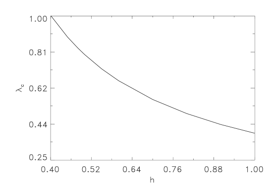
Figure 5: $\lambda_{c}$ vs. $h$ parameter of diffusivity. For small $h$ values $\lambda_{c}$, and hence the noise intensity, increase monotonically.

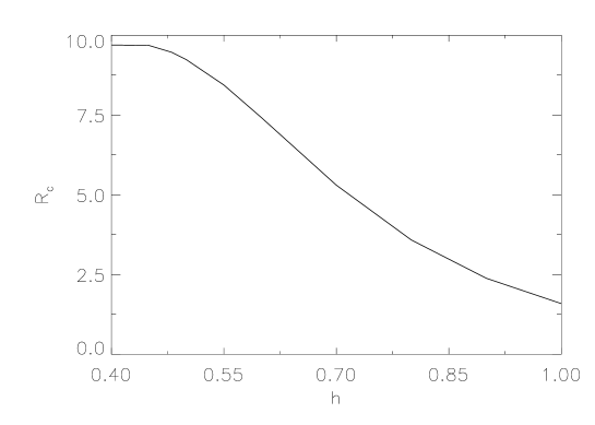
Figure 6: Signal-to-noise ratio at $\lambda_{c}$ vs. $h$. We can see a saturation phenomena as $h$ decreases.

IV Conclusions

The study of SR in extended or coupled systems, motivated by both, some experimental results and the technological interest, has recently attracted considerable attention extend1 ; otros ; extend2 ; extend2b ; extend3a ; extend3b . In some previous papers extend2 ; extend2b ; extend3a ; extend3b we have studied the SR phenomenon for the transition between two different patterns, exploiting the concept of nonequilibrium potential GR ; I0 . In this work we have analyzed the SR phenomenon in an extended system from a different point of view, that is studying SR between two noise-induced patterns ga93 ; nsp .

Some related work correspond to the misleadingly called double stochastic resonance ZKSG , as well as to a previous work MGOC that is tightly related to noise-induced phase transitions nipt1 ; nipt2 . In both cases the authors have resorted to a standard mean-field approach. Here we adopt a different approach, obtaining numerically the exact form of the noise-induced patterns (both the stable and unstable ones) as well as the analytical expression of the nonequilibrium potential. In this way we were able to obtain the transition rates and clearly quantify the SR phenomenon by means of the SNR.

We have seen that the a nonhomogeneous spatial coupling, through density-dependent diffusivity, changes the effective dynamics of the system and, in agreement with extend3c , that such nonhomogeneity could contribute to enhance the SR phenomenon. The form of the patterns, position of the attractors, barrier’s high, explicitly depend on the noise intensity. We have found that there are ranges or windows of noise intensities where the phenomenon could arise (reentrance).

By considering the adiabatic limit and exploiting the two-state approximation we have theoretically predicted the occurrence of SR between those noise-sustained patterns. It is worth here remarking that it is the same noise source the one that sustains the patterns and induces SR for transitions among them. The maximum of the SR response occurs in the symmetric case, in agreement with the results found in extend3a ; extend3b . The SR phenomenon is robust respect to variations of the $h$ parameter of diffusivity, and when $h$ decreases the SNR maximum increases and shifts toward higher $\lambda$ values. The last fact follows from the associated shift of the noise-induced transition to larger noise intensities which take place in the spatially uncoupled associated system (i.e. the 0-d system resulting from suppressing the gradient term in Eq.(3)).

The consideration of more general forms of couplings in many component systems will allow us to analyze SR between noise-induced patterns in activator-inhibitor-like systems. We will also study, within the present framework, the competence between local and non-local spatial couplings extend2b ; extend3b , etc. These aspects, together with Monte Carlo simulations of the different cases, will be the subject of further work.