Optimal switching policies using coarse timesteppers.

Abstract

We present a computer-assisted approach to approximating coarse optimal switching policies for systems described by microscopic/stochastic evolution rules. The “coarse timestepper” constitutes a bridge between the underlying kinetic Monte Carlo simulation and traditional, continuum numerical optimization techniques formulated in discrete time. The approach is illustrated through a simplified kinetic Monte Carlo simulation of $NO$ reduction on a $Pt$ catalyst: a switch between two coexisting stable steady states is implemented by minimal manipulation of a system parameter.

1 Introduction

The search for optimal time-varying operation protocols for chemically reacting systems has remained an exciting research subject for many decades. It has been receiving increased attention recently, both for lumped and distributed in space systems (e.g. [17, 1]); as sensing and actuation become increasingly more resolved in space and time, spatiotemporally complicated operating policies can be considered (e.g. [19]). Proposed computational approaches may involve (a) solution of the temporally discretized problem (both for the process and for the operating variable(s)) simultaneously, using large sparse linear algebra techniques (e.g [17]); (b) formulations involving direct integration of the model equations in time, keeping track of possible constraint violations [18, 2]; or dynamic programming formulations. Knowledge of a macroscopic process model, in the form of macroscopic mass balances closed through appropriate constitutive expressions -such as chemical kinetic rate formulas-, is a fundamental prerequisite for these computational solution strategies.

In contemporary engineering modeling, however, we are often faced with problems for which the available physical description is in the form of atomistic / stochastic evolution rules (kinetic Monte Carlo, Lattice Boltzmann, molecular dynamics, Brownian dynamics) while the design, optimization or control is required at a coarse-grained, macroscopic level. Over the last few years we have been developing a computational approach enabling microscopic / stochastic simulators to directly perform system-level tasks, such as coarse integration, stability analysis, bifurcation/continuation[16, 3, 9] and feedback control [14], thus circumventing the derivation of explicit macroscopic evolution equations.

Here we demonstrate the extension of this computational enabling technology to coarse optimization tasks. In particular, we computationally approximate coarse optimal switching policies for (the expected behavior of) a kinetic Monte Carlo simplified model of a catalytic chemical reaction. The system is characterized by two “coarse-grained” stable stationary states. We seek optimal (for a particular definition of the cost function) parameter variation policies that will switch the kinetic Monte Carlo simulation from one steady state to the other within a finite time interval.

2 Process description

We investigate microscopic/stochastic processes for which we believe that the coarse-grained, expected dynamics can be adequately approximated by a model of the general type

$$\dot{x}=F(x,p)$$ (1)

but where the right-hand-side of the evolution law, $F$, is not available in closed form. Here, $x(t)\in{\rm I}\!{\rm R}^{n}$ is a state variable vector, $t$ is the time, $\dot{x}$ is the time derivative of $x$, $\displaystyle{\frac{dx}{dt}}$, and $p\in{\cal P}^{m}$ is the vector of process parameters (${\cal P}^{m}\subset{\rm I}\!{\rm R}^{m}$ is the subset of available values of the process parameters). The state variables $x(t)$ are typically a few lower order moments of an atomistically evolving distribution (e.g. a concentration, or, in our example, a surface coverage, the zeroth moment of the distribution of adsorbates on the surface). The (unavailable) equation for the expected behavior of the process may possess, at fixed process parameter values, one or more steady states $x_{ss,i}$.

2.1 The coarse timestepper

The basis of our approach is the computation of a deterministic optimal policy for the expected dynamics of the process (the “coarse-grained dynamics”) circumventing the derivation of a closed form evolution equation for these dynamics. This deterministic policy for the coarse-grained behavior will then be applied to individual realizations of the process. As we will explain below, it is convenient in our approach to reformulate the coarse dynamics in discrete rather than continuous time. The coarse evolution law then takes the form:

$$\begin{array}[]{l}x_{i+1}=G_{T}(x_{i},p(t)),\quad t\in(t_{i},t_{i}+T]\vspace{2mm}\\ \end{array}$$ (2)

where $x_{i}$ is the state at the beginning of $i$-th time interval, $t_{i}$, $T$ is the time interval duration (reporting horizon), $G_{T}$ represents the evolution of Eq.1 for a process parameter profile $p(t)$, initialized at $x_{i}$ and evolved for time $T$, arriving at state $x_{i+1}$ at $t_{i}+T\equiv t_{i+1}$.

Conventional algorithms for the solution of optimization problems involving $G_{T}$ incorporate frequent calls to a subroutine that evaluates $G_{T}$ and/or the action of its derivatives on initial conditions. Equation-free based algorithms estimate the same quantities by short bursts of (possibly ensembles of) microscopic simulations conditioned on the same macroscopic initial conditions. The coarse time-stepper constitutes such an estimate of the discrete-time, macroscopic input-output map $G_{T}$ obtained via the kinetic Monte Carlo simulator. Through a lifting operator the macroscopic initial condition is translated into several consistent microscopic initial conditions (distributions conditioned on a few of their lower moments). This ensemble of microscopic initial conditions is then evolved microscopically, in an easily parallelizable fashion (one consistent realization per CPU). The results are averaged through a restriction operator back to a macroscopic “output”; it is precisely this output that traditional algorithms simply compute through function evaluations when the evolution equations are available in closed form. As extensively discussed in [11, 9], part of the microscopic evolution is spent in a “healing” process - the higher moments, which have been initialized “wrong” quickly relax to functionals of the low order moments (our state variables). A separation of time scales (fast relaxation of the high moments to functionals of the low ones, and slow -deterministic- evolution of the low ones) underpins the existence of a deterministic coarse grained evolution law. The dynamics of the evolving microscopic distribution moments constitute thus a singularly perturbed system. The requirement of finite time microscopic evolution (necessary to the moment healing process) conforms with the discrete-time formulation of the coarse optimization problem, which is common in many optimization algorithms (see section 3 below).

2.2 Numerical experiment

We illustrate the proposed combination of traditional optimization techniques with stochastic simulators through a kinetic Monte Carlo realization (using the stochastic simulation algorithm, proposed by Gillespie [4, 5]) of a drastically simplified kinetic model of $NO$ reduction by $H_{2}$ on Pt surfaces:

$${\frac{d\theta}{dt}}=\alpha(1-\theta)-\gamma\theta-k(1-\theta)^{2}\theta.$$ (3)

Here $\theta$ describes the surface coverage of adsorbed $NO$, $\alpha$, $\gamma$ are the $NO$ adsorption and desorption rate constants respectively, and $k$ is the reaction rate constant. The reaction term is third order due to the need for two free adjacent sites for the adsorption of $H_{2}$. In Figure 1 we present the deterministic bifurcation diagram in the form of coverage $\theta_{ss}$ at steady-state as a function of $k$ for $\alpha=1$ and $\gamma=0.01$. We observe a range of $k$ values for which the system exhibits multiple steady-states; the higher and lower ones are locally stable, while the middle one is unstable.

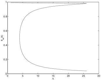
Figure 1: Bifurcation diagram of $\theta$ at steady state with respect to $k$.

A description of the use of the coarse KMC timestepper in obtaining “coarse” versions of this bifurcation diagram may be found in [11].

3 Coarse computational optimization

Computing the temporal profiles of the process parameters that cause the transition of the coarse-grained system from an initial stationary state to a different final one can be formulated as an optimization problem; the objective is to minimize an integral cost function over time:

$${\min_{p(t)\in{\cal P}^{m}}}\displaystyle{\int_{0}^{\infty}}{\cal Q}(t,x,p)dt$$ (4)

where ${\cal Q}$ is a continuous scalar cost function. The constraints for this coarse optimization problem are the (unavailable) coarse process evolution equations Eq.1, the initialization at one of the coarse stationary states for $p=p_{ss}$, the requirement of termination at a different stationary state for the same process parameter value $p_{ss}$, as well as, possibly, other inequality constraints $g(x,p)$:

$$\begin{array}[]{c}\dot{x}-F(x(t),p(t))=0,\quad g(x,p)\leq 0\vspace{2mm}\\ \begin{array}[]{ll}p(0)=p_{ss},&\displaystyle{\lim_{t\rightarrow\infty}}p(t)=p_{ss}\vspace{2mm}\\ x(0)=x_{ss,1},&\displaystyle{\lim_{t\rightarrow\infty}}x(t)=x_{ss,2}\end{array}\end{array}$$ (5)

This is an infinite dimensional problem in continuous time. Direct solution methods are based on the calculus of variations. Semi-infinite programming approaches provide us with the necessary mathematical tools to solve such problems with finite time horizon [6], through discretization of the temporal domain.

Another approach consists of approximating this problem through a finite time horizon problem with a final state penalty, which is (in our case) subsequently solved in discrete time. This results in a finite dimensional, generally nonlinear, optimization problem which -if the coarse equations are available- could be solved using available optimization techniques. For example, discretizing the process time $[0,t_{f}]$ in $N$ time intervals of length $T$ (not necessarily constant) and assuming that the process parameters remain constant within each interval $p(t)=p_{i+1},\;\forall t\in(t_{i},t_{i}+T]$, results in the following optimization program with $(N+1)\times n+N\times m$ variables and $n\times(N+1)+m$ equality constraints:

$$\begin{array}[]{c}\begin{array}[]{r@{}l}\displaystyle{\min_{p_{i}\in{\cal P}^{m}}}&\displaystyle{\sum_{i=1}^{N}}\displaystyle{\int_{(i-1)T}^{iT}}{\cal Q}_{d}(t,x_{i},x_{i-1},p)dt\vspace{2mm}\\ &+{\cal W}(R(|x_{N}-x_{ss,2}|-\epsilon))\end{array}\vspace{2mm}\\ {\rm s.t.\vspace{2mm}}\\ g_{d}(x_{0},\dots,x_{N},p)\leq 0,\vspace{2mm}\\ x_{i}=G_{T}(x_{i-1},p)=0,\quad i=1,\dots,N,\quad x_{0}=x_{ss,1}\vspace{2mm}\\ p(t)=\displaystyle{\sum_{i=1}^{N}p_{i}\Pi(\frac{t}{T}-i-\frac{1}{2})}+p_{ss}H(-t).\end{array}$$ (6)

Here ${\cal Q}_{d}$ is analogous to the ${\cal Q}$ function for the discrete values of the state, $g_{d}$ is similarly analogous to $g$, ${\cal W}(\cdot)$ is a class $K$ scalar function, $R(\cdot)$ is the ramp function and $\epsilon$ is a value for which $|x_{N}-x_{ss,2}|\leq\epsilon<=>{\cal W}=0$, $\Pi(\cdot)$ is the standard boxcar function and $H(\cdot)$ denotes the Heaviside function. Appropriate final state penalty contributions to the cost function take the place of final state constraints at infinite time as stated in the original formulation of the problem; the final state is restricted to be (in finite time) within a neighborhood of the final stationary state. This fully discrete-time formulation is ideally suited for linking with a coarse timestepper. The optimization problem formulated in Eq.6 can further be reduced in size by discretizing only the process parameter temporal behavior, resulting in the following formulation (coined control vector parameterization [18]) with $N\times m$ variables and $m$ equality constraints:

$$\begin{array}[]{c}\begin{array}[]{r@{}l}\displaystyle{\min_{p_{i}\in{\cal P}^{m}}}&\displaystyle{\sum_{i=1}^{N}}\displaystyle{\int_{(i-1)T}^{iT}}{\cal Q}_{d}(t,x_{i},x_{i-1},p)dt\vspace{2mm}\\ &+{\cal W}(R(|x_{N}-x_{ss,2}|-\epsilon))\end{array}\vspace{2mm}\\ {\rm s.t.\vspace{2mm}}\\ g_{d}(x_{0},\dots,x_{N},p)\leq 0,\vspace{2mm}\\ p(t)=\displaystyle{\sum_{i=1}^{N}p_{i}\Pi(\frac{t}{T}-i-\frac{1}{2})}+p_{ss}H(-t)\vspace{2mm}\\ {\rm where\vspace{2mm}}\\ x_{i}=G_{T}(x_{i-1},p)=0,\quad i=1,2,\dots,N\vspace{2mm}\\ x_{0}=x_{ss,1}.\end{array}$$ (7)

The difference with the previous formulation lies in that the variables $x_{i},\;\;i=1,\dots,N$ are solved for internally, to reduce the size of the optimization problem. In cases where the explicit form of Eq.1 is unavailable, the state evolution is provided through direct simulation of the system.

3.1 Solution methodology

Traditional discrete time optimization schemes would call, during the solution process, a numerical integration subroutine for the system equations (and possibly variational integrations for the estimation of derivatives). This call is now substituted by the coarse timestepper; the most important numerical issue is that of noise, inherent in the lifting process and the stochastic simulations, and the variance reduction necessary to estimate the state or its various derivatives. Simulations of different physical size systems (different lattice sizes in our simulation) are characterized by different levels of noise, while the expectation asymptotically approaches a limiting value for infinite system size. For the type of simulations in this paper, changing the physical size of the simulated domain on the one hand, and changing the number of copies of the simulation on the other, have comparable effects in reducing the variance of the simulation output; this, however, is not generally the case in KMC simulations. When a switching policy for a particular physical size system is required (e.g. for nanoscopic reacting systems, such as the chemical oscillations on Field Emitter tips [15]) variance reduction can be affected through a larger ensemble of consistent microscopic initializations (see also [12] for a variance reduction technique using stochastic calculus). Simulation noise affects both function evaluations and (numerical) coarse derivative evaluations, and thus becomes an important element of the approach. It is interesting, however, to observe that massively parallel computation can reduce the wall clock time required for the computation distributing different microscopic initializations to different CPUs.

Due to the presence of noise in the coarse timestepper results, the use of optimization algorithms that are specifically designed to be insensitive to noise becomes necessary (it is well known that the numerical estimation of derivatives is highly susceptible to noise). A class of direct search algorithms that fulfill this criterion are ones that use only function evaluations to search for the optimum such as iterative dynamic programming [13], Luus-Jaakola [10], Nelder-Mead and Hooke-Jeeves algorithms. Algorithms that compute local and bounded approximations of the Jacobian matrix of the cost function with respect to the process parameters have also been developed, such as the implicit filtering algorithm. The reader may refer to [8] for a review of these methods.

In all the above iterative algorithms, an appropriate initial guess of the process policy profile and a set of search directions for the $m\times N$ variables is required. The usual set of search directions (also used in our numerical experiment) is the unitary basis for ${\rm I}\!{\rm R}^{m\times N}$. The components of the search algorithms also include a vector, the elements of which are the maximum distances the algorithm should venture from the current position during the new direction search step at each iteration. These perturbation distances are called scales, and appear in decreasing order.

Selection of the scales in the search algorithm requires estimates of the noise magnitude. A scale that is too small not only leads to increased computation time with no apparent advantages, but, especially in the case of algorithms that compute approximations of the Jacobian, can lead to grossly erroneous results for the search. The following timestepper protocol yields, in our case, simulation results of known variance magnitude:

1. Initialize timestepper. Set:

   • lattice size $N_{l}$,

   • solutions sampling size $M_{r}$,

   • variance metric $d$ as the square root of the variance, subsequently divided by the average value of the sample.

   • variance magnitude limit $d_{max}$ and

   • maximum sample size $M_{max}$.

2. In each time step, the timestepper:

   1. simulates system for the desired parameter value $M_{r}$ times (this can be affected through different microscopic initializations and/or different random seeds in the Monte Carlo process) and computes $d$.

   2. If $d>d_{max}$ and $M_{r}<M_{max}$, increases $M_{r}$, repeat step (a)

   3. If $d\leq d_{max}$ and $M_{r}>M_{min}$ decreases $M_{r}$, continue with next time step.

Adaptively adjusting the ensemble of realizations thus helps in the choice of scales. Optimization algorithms that are based only on function evaluations are not guaranteed to converge to a global minimum, or even to a minimum. This is due to the fact that we do not compute the necessary optimality conditions in the neighborhood of the result, and also because a search direction may have been neglected. Once the optimization algorithm has converged and produced a policy profile, it is prudent to restart it with initial guess the result of the previous search. This causes a large perturbation, which may lead to a better optimum. Once two consecutive runs have produced the same result, the free variable profile is declared “optimal over all scales” [8].

4 Numerical Results

The approach outlined in the previous section was applied towards the computation of an optimal switching policy (between different stationary states) in our simplified $NO$ reduction model. Specifically, our objective is to switch from the $\theta_{ss,s}$, to the $\theta_{ss,f}$ locally stable stationary states (traversing the unstable stationary state $\theta_{ss,i}$) with the minimum possible effort. The cost function in Eq.7 was (somewhat arbitrarily) defined as:

$$\begin{array}[]{l}{\cal Q}=(k(t)-k_{ss})^{2}(1-0.3e^{-t})T(\displaystyle{\sum_{i=0}^{N}}\delta(t-iT))\vspace{2mm}\\ {\cal W}=50[1-exp(R(|\theta(t_{N})-\theta_{ss,f}|-\epsilon))]\end{array}$$

where $\epsilon=0.05$ and $R$, $\delta$ denote the ramp and Dirac function respectively. We assume that the single “manipulated variable” for this problem (the process parameter $p$ of Eq.1) is the reaction rate constant $k$. The process parameters used for the specific optimization problem are presented in Table 1.

Table 1: Process parameters

Parameter	Value	Steady states
$T$	0.25	$\theta_{ss,s}$	0.3301
$N$	20	$\theta_{ss,i}$	0.6803
$t_{f}$	5	$\theta_{ss,f}$	0.9896
$k_{ss}$	0.45
$\alpha$	1.0
$\gamma$	0.01

KMC simulations based on the Gillespie algorithm formed the basis of the coarse time-stepper that was used to estimate the coarse system response. A variety of lattice and sample sizes were used in estimating the dynamic behavior of the system. Hooke-Jeeves was the algorithm we chose to search for the optimal profile. In Table 2 we present the value of the cost function for the computed optimal parameter profiles, through which the effect of the error in the computed optimal profile is implicitly quantified. As the lattice size $N_{l}$ increases the KMC simulations expected profiles asymptotically converge to the profile obtained at the limit. For the simulations presented the expectation dependence to $N_{l}$ was insignificant. A secondary advantage of the increased lattice size was the variance reduction since $d\propto N_{l}^{-1/2}$. This leads, at large $N_{l}$, to results from the search for the optimal profile of $k$ that are closer to ones obtained when we use the timestepper of the actual deterministic problem (for comparison purposes). The main variance reduction parameter in the presented simulations was the sample size $M_{r}$ used to compute the coarse response; when $M_{r}$ increases in the KMC simulations, the noise magnitude $d$ decreases, as expected, since $d\propto M_{r}^{-1/2}$.

Table 2: Hooke-Jeeves search results

Model Lattice Runs Objective t∗ [s] Legacy $-$ $-$ 10.3709 129 KMC $100\times 100$ $200$ 10.5418 674 KMC $200\times 200$ $400$ 10.4155 4673 KMC $300\times 300$ $600$ 10.3973 16300 KMC $400\times 400$ $800$ 10.3815 38469 KMC $500\times 500$ $1000$ 10.3811 75307

∗ single CPU pentium $IV$ at $2.4\;GHz$

The Gillespie algorithm was chosen so that the coarse behavior is known at the large system size limit, and the noisy timestepper optimization results can be compared to it. The objective value convergence to the computed optimal value from the ODE “direct simulator” comes at the cost of increased computational work. The use of parallel computing can, as we discussed, drastically decrease the necessary wall clock time. In Figure 2 we present the results for $N_{l}=500\times 500$ and $M_{r}=1000$ and compare them to the direct ODE simulation results. A near-optimal parameter profile is arrived at, due to the combination of MC simulations’ noise, system size, and the Hooke-Jeeves search algorithm (a search direction that has been investigated and characterized as unfavorable is not reinvestigated to conserve CPU time).

a)

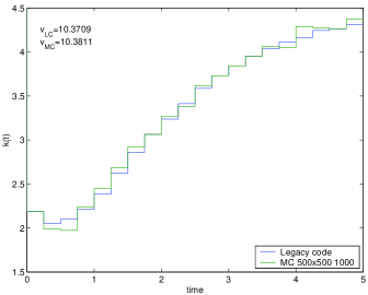
b)

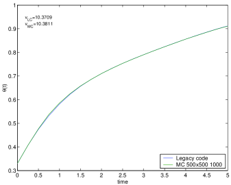
Figure 2: Results using Hooke-Jeeves algorithm through numerical integration of Eq.1 (blue line) and using KMC simulation (green line), a) Optimal temporal profile of process reaction rate $k$, b) Evolution of $NO$ coverage $\theta$.

We also used Implicit Filtering to compute a near optimal steady state switching profile for $k$. The method of implicit filtering uses consecutive bounded approximations of the Jacobian with variable step and limit to the maximum change of the design variable at each iteration. The timestepper protocol used had $d_{max}=0.005$, $N_{max}=16N_{l}$, $M_{max}=4M_{r}$, $N_{l}=126\times 126$ and $M_{r}=252$ and by adaptively adjusting $M_{r}$ the noise magnitude criterion was satisfied. The resulting near optimal time profile of $k(t)$ is presented in Figure 3a, while the near optimal path of $NO$ coverage evolution $\theta(t)$ is shown in Figure 3b for an averaged realization, and in Figure 3c for a single KMC realization with lattice size $N_{l}=100\times 100$ and reporting horizon $\delta t=0.0039$.

Table 3: Implicit Filtering search results

Model $d_{max}$ Scales Objective t∗ [s] Legacy $-$ $-$ 10.3709 168 KMC $0.005$ $2^{-0},\dots,2^{-3}$ 10.5461 297 KMC $0.005$ $2^{-0},\dots,2^{-4}$ 10.7922 282 KMC $0.0005$ $2^{-3},\dots,2^{-5}$ 10.4110 3684 KMC $0.001$ $2^{-0},\dots,2^{-4}$ 10.4129 6858

∗ single CPU pentium $IV$ at $2.0\;GHz$

In Table 3 we present computational results obtained through incorporating the coarse timestepper in an implicit filtering algorithm. We also observe that a good scales selection depends heavily on $d_{max}$, as scales below a certain limit have an adverse effect on the computed near optimal path result (compare the results of the search when the lowest scale is $2^{-4}$ to $2^{-3}$).

Our timestepper protocol can be combined with the search algorithm to solve successively the optimization program using more refined scales. Specifically, an initial search, with large values for the scales, can take place at higher $d_{max}$, followed by searches with gradually lower $d_{max}$ and smaller scales to refine the search for the optimal path; this approach may lead to computational savings. When using the KMC with $d_{max}=0.005$ and a lower scale of $2^{-3}$ for an initial search, followed by a KMC simulation of the system with $d_{max}=0.0005$ and lower scale of $2^{-5}$, we find a near optimal path with $v=10.4110$ in a total time of $3981\;s$. A search using KMC with $d_{max}=0.001$ and lower scale of $2^{-4}$ lead to computing a near optimal path of $v=10.4129$ in $6858\;s$ (the results are shown in Table 3).

The optimal switching path, shown in figure 3b, takes the (expected) phase point from $\theta_{ss,s}$ through the unstable stationary state $\theta_{ss,i}$ as shown in Figure 3b. After this is accomplished, we observe that the optimal k(t) trajectory rapidly converges back to $k_{ss}$ (see Figure 3a). The coarse phase point is now within the region of attraction of the steady state $\theta_{ss,f}$, and no particular switching action is needed to get us there.

The cost function values presented in this section were computed, for reference purposes, by integrating the coarse system Eq.3 for the optimal switching profile found. During the optimal search using KMC simulations, the coarse process model was never used. Several optimization algorithms were explored in conjunction with the coarse timestepper, including Hooke-Jeeves, Nelder-Mead, Implicit-Filtering as well as Multilevel Coordinate Search (MCS). Hooke-Jeeves was primarily chosen due to the simplicity of the method and its relative convergence speed. The Implicit Filtering algorithm was mainly used with the coarse timestepper noise-reduction protocol. Enforcing an upper bound on the noise magnitude, along with the selection of the value of the scales provided an order of magnitude estimate of the error in the estimated derivatives during the Jacobian approximation.

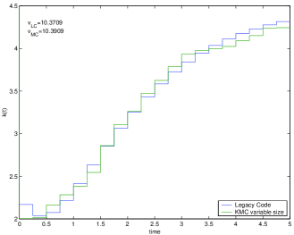
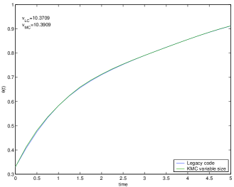
a) b) c)

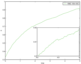
Figure 3: Results using Implicit Filtering algorithm through numerical integration of Eq.1 (blue line) and using KMC simulation (green line), a) Optimal temporal profile of process reaction rate $k$, b) Evolution of $NO$ coverage $\theta$, c) Evolution of $NO$ coverage $\theta$ for a single KMC realization, $N_{l}=100\times 100$, $\delta t=0.0039$.

5 Conclusions

We presented a computational methodology for the location of coarse near-optimal parameter policies (in particular, steady state switching policies) for systems for which macroscopic, coarse evolution equations exist but are not available in closed form. The advantage of the proposed method lies in the establishment, through the coarse timestepper, of a computational bridge between atomistic/ stochastic simulators and traditional (in particular, derivative free) optimization algorithms. The approach can be directly extended to systems with higher dimensional expected behavior (see for example [11]), and possibly, through matrix-free methods, to systems with infinite dimensional (spatially distributed, but dissipative) expected behavior [3]. Our current efforts focus on applying this methodology to the study of rare events and coarse optimal paths in computational chemistry (e.g. [7]).

References

- [1] A. Armaou and P. D. Christofides. Optimization of dynamic transport-reaction systems using nonlinear model reduction. Chem. Eng. Sci., 57:5083–5114, 2002.
- [2] T. Binder, A. Cruse, C. A. C. Villar, and W. Marquardt. Dynamic optimization using a wavelet based adaptive control vector parameterization strategy. Comput. Chem. Eng., 24:1201–1207, 2000.
- [3] C. W. Gear, I. G. Kevrekidis, and C. Theodoropoulos. “coarse” integration/bifurcation analysis via microscopic simulators: micro-Galerkin methods. Comp. Chem. Engng., 26:941–963, 2002.
- [4] D. T. Gillespie. A general method for numerically simulating the stochastic time evolution of coupled chemcial reactions. J. Comp. Phys., 22:403–434, 1976.
- [5] D. T. Gillespie. A rigorous derivation of the chemical master equation. Physica A, 188:404–425, 1992.
- [6] R. Hettich and K. O. Kortanek. Semi-infinite programming: Theory, methods, and applications. SIAM Review, 35:380–429, 1993.
- [7] G. Hummer and I. G. Kevrekidis. Coarse molecular dynamics of a peptide fragment: free energy, kinetics and long time dynamics computations. J. Chem. Phys., 118:10762–10773, 2003.
- [8] C. T. Kelley. Iterative Methods for Optimization, volume 18 of Frontiers in Applied Mathematics. SIAM, Philadelphia, USA, 1999.
- [9] I. G. Kevrekidis, C. W. Gear, J. M. Hyman, P. G. Kevrekidis, O. Runborg, and K. Theodoropoulos. Equation-free multiscale computation: enabling microscopic simulators to perform system-level tasks, submitted. Comm. Math. Sciences, 2002.
- [10] R. Luus and T. H. I. Jaakola. Optimization by direct search and systematic reduction of the size of search region. AIChE J., 19:760–766, 1973.
- [11] A. G. Makeev, D. Maroudas, and I. G. Kevrekidis. “Coarse” stability and bifurcation analysis using stochastic simulators: Kinetic Monte Carlo examples. J. Chem. Phys., 116:10083–10091, 2002.
- [12] M. Melchior and H. C. Oettinger. Variance reduced simulations of stochastic differential equations. J. Chem. Phys., 103:9506–9509, 1995.
- [13] A. Rusnak, M. Fikar, M. A. Latifi, and A. Meszaros. Receding horizon iterative dynamic programming with discrete time models. Comp. & Chem. Eng., 25:161–167, 2001.
- [14] C. I. Siettos, A. Armaou, A. G. Makeev, and I. G. Kevrekidis. Microscopic/stochastic timesteppers and coarse control: a kinetic Monte Carlo example. AIChE J., 49:1922–1926, 2003.
- [15] Y. Suchorski, J. Beben, E. W. James, J. W. Evans, and R. Imbihl. Fluctuation-induced transitions in a bistable surface reaction: Catalytic CO oxidation on a Pt field emitter tip. Phys. Rev. Lett., 82:1907, 1999.
- [16] K. Theodoropoulos, Y.-H. Qian, and I.G. Kevrekidis. “coarse” stability and bifurcation analysis using timesteppers: a reaction diffusion example. Proc. Natl. Acad. Sci., 97:9840–9843, 2000.
- [17] S. Vasantharajan, J. Viswanathan, and L. T. Biegler. Reduced successive quadratic programming implementation for large-scale optimization problems with smaller degrees of freedom. Comput. Chem. Eng., 14:907–915, 1990.
- [18] V. S. Vassiliadis, R. W. H. Sargent, and C. C. Pantelides. Solution of a class of multistage dynamic optimization problems, parts I & II. Ind. & Eng. Chem. Res., 33:2111–2133, 1994.
- [19] J. Wolff, A. G. Papathanasiou, I. G. Kevrekidis, H. H. Rotermund, and G. Ertl. Spatio-temporally addressing surface activity. Science, 294:134–137, 2001.