Hamiltonian Hopf bifurcations in the discrete nonlinear Schrödinger trimer: oscillatory instabilities, quasiperiodic solutions and a ’new’ type of self-trapping transition

Abstract

Oscillatory instabilities in Hamiltonian anharmonic lattices are known to appear through Hamiltonian Hopf bifurcations of certain time-periodic solutions of multibreather type. Here, we analyze the basic mechanisms for this scenario by considering the simplest possible model system of this kind where they appear: the three-site discrete nonlinear Schrödinger model with periodic boundary conditions. The stationary solution having equal amplitude and opposite phases on two sites and zero amplitude on the third is known to be unstable for an interval of intermediate amplitudes. We numerically analyze the nature of the two bifurcations leading to this instability and find them to be of two different types. Close to the lower-amplitude threshold stable two-frequency quasiperiodic solutions exist surrounding the unstable stationary solution, and the dynamics remains trapped around the latter so that in particular the amplitude of the originally unexcited site remains small. By contrast, close to the higher-amplitude threshold all two-frequency quasiperiodic solutions are detached from the unstable stationary solution, and the resulting dynamics is of ’population-inversion’ type involving also the originally unexcited site.

1 Introduction

As indicated by a number of recent results (e.g. [1, 2, 3, 4, 5, 6, 7, 8, 9]), oscillatory instabilities of time-periodic solutions in Hamiltonian anharmonic lattice models are quite ubiquitous, and likely to play an important role in the dynamics of any physical system which, in some approximation, can be described by such a model. Typically they are associated with an inhomogeneous amplitude distribution of the solution dividing the lattice into two sublattices of small- and large-amplitude sites, respectively, and oscillatory instabilities appear when internal oscillations of the sublattices resonate.

As long as the harmonic coupling is not too strong, time-periodic solutions for coupled anharmonic oscillators can be conveniently described using the multibreather formalism [10, 11], utilizing the (’anticontinuous’) limit of zero coupling to identify each solution with a coding sequence. In the simplest case of time-reversible solutions with one single determination of the oscillation pattern for the individual uncoupled oscillators at a given period, the code is defined as +1 for each site oscillating with a certain reference phase, -1 for each site oscillating with the opposite phase, and 0 for each site at rest. (This scheme can be readily generalized to include e.g. higher-harmonic oscillations by allowing codes $\pm 2,\pm 3,...$, or non-time-reversibility by allowing arbitrary phase torsions [11]). This identification is unique for sufficiently weak coupling [10, 11], and can be obtained by numerical continuation using Newton-type schemes (e.g. [12]).

In particular, for Klein-Gordon (KG) chains of harmonically coupled soft anharmonic oscillators, most known examples of oscillatory instabilities are associated with solutions whose coding sequences contain blocks of the kind $...,1,0^{p},-1,0,...$, with integer $p\geq 0$ ($0^{p}$ means 0 repeated $p$ times). (For hard oscillators, a corresponding statement is true provided that the code sequence is multiplied with $(-1)^{n}$.) Thus, large-amplitude sites of alternating phases (codes $\pm 1$) and small-amplitude sites (code $0$) provide a two-sublattice structure. Generically, such solutions are linearly stable for weak coupling when the internal oscillation frequencies for the two sublattices are separated, but for larger coupling the frequencies may overlap causing resonances and instabilities. By contrast, blocks of the kind $...,1,0^{p},1,0,...$ typically yield nonoscillatory instabilities already for weak couplings. This difference can be related to the different natures of extrema for a corresponding effective action, defined in [11] as a function of the individual phases at each site (see also [13, 14, 3], and [15] for further developments).

Oscillatory instabilities were explicitly demonstrated e.g. for: (i) two-site out-of-phase breathers [1, 14] (’twisted localized modes’ [16, 5]) with code $...0,0,1,-1,0,0...$; (ii) discrete dark solitons [3, 17, 7] (’dark breathers’ [9]) with a hole and a phase shift added to a stable background wave, code $...1,-1,1,-1,0,1,-1,1,-1...$; (iii) nonlinear standing waves [4, 7, 8], corresponding to periodic or quasiperiodic repetitions of blocks of codes of type $\{1,0^{p},-1,0^{q}\}$ with particular combinations of integers $p,q\geq 0$. These instabilities may play an important role in the processes of breather formation and evolution to energy equipartition [7, 8]. Oscillatory instabilities are found also e.g. for two-dimensional vortex-breathers [13, 18, 6].

Mathematically, oscillatory instabilities appear through ’Krein collisions’ (e.g. [19]) of eigenvalues to the corresponding linearized equations of opposite Krein (symplectic) signatures. Although well-known from other branches of physics, their relevance for the dynamics of anharmonic lattices was realized mainly after [11]. Generally linear stability of time-periodic solutions is studied through the linearization of a Poincaré return map with the exact solution as a fixed point (Floquet map), and its symplectic nature implies that all eigenvalues (Floquet multipliers) must lie on the unit circle for stability. In a Krein collision, four eigenvalues leave the unit circle as a complex quadruplet.

However, for weakly coupled KG lattices the small-amplitude dynamics can be approximated, through a multi-scale expansion (e.g. [21, 7]), by a discrete nonlinear Schrödinger (DNLS) equation. A time-periodic KG solution then becomes a purely harmonic (stationary) DNLS solution, which can be made time-independent by studying the dynamics in a frame rotating with this frequency. Thus, performing also the stability analysis in the rotating frame reduces the problem to studying stability of (relative) equilibria, as no explicit time-dependence appears in the linearized equations [23, 24]. Linear stability demands all eigenvalues of the linearized flow to lie on the imaginary axis, and a Krein collision manifests itself as two pairs of complex conjugated imaginary eigenvalues with opposite Krein signature colliding and going out in the complex plane as a quadruplet (e.g. [25]). This collision is also (e.g. [27, 28]) referred to as a 1:-1 resonance (equal frequencies, opposite Krein signatures), and corresponds to a bifurcation of two (relative) time-periodic solutions which, due to its similarity to a Hopf bifurcation in dissipative systems, has been termed [29] a Hamiltonian Hopf (HH) bifurcation.

Following a recent description of the essential aspects of the HH bifurcation [30], we briefly recall its phenomenology (see [27, 28] for a rigorous description). HH bifurcations may be of two different types called [30] ’type I’ and ’type II’, respectively (in a related context, these bifurcation classes were called [31] ’hyperbolic regime’ and ’elliptic regime’, respectively, referring to the nature of the corresponding normal forms). In the type I bifurcation, two (’Lyapunov’) families of stable periodic solutions surround the equilibrium in its stable regime, merge at the bifurcation point, and form a single family detached from the equilibrium in its unstable regime. For type II, the two periodic solutions belong to a single connected family on the stable side of the bifurcation, which shrinks to a fixed point and disappears on the unstable side. Thus, while for type I stable periodic solutions exist close to (but away from) the equilibrium also in its unstable regime, for type II no periodic solutions exist close to the unstable equilibrium. Since for the DNLS equation this description refers to the rotating frame, the (relative) equilibria correspond to time-periodic stationary solutions and the (relative) periodic solutions generally to quasiperiodic two-frequency solutions in the original frame. For the DNLS equation (and other equations with particular symmetries [33]) such quasiperiodic solutions may persist, and even be spatially localized, also for infinite lattices [10, 14, 5].

It is our purpose to describe, mainly by numerical means, the nature of these bifurcations, aiming at an increased understanding for the dynamics in the oscillatory instability regime. We focus here on the simplest possible model where the above described mechanism for oscillatory instabilities can occur: the 3-site DNLS-model with periodic boundary conditions and the stationary solution with code $+1,-1,0$. The fact that this solution exhibits a complex instability is known already since the pioneering works of Eilbeck et.al. [23, 24]; however, in spite of the wealth of existing literature on this model (e.g. [23, 24, 34, 35, 36, 38, 40, 41, 42] and references therein), apparently the unstable dynamics of these stationary states and the properties of the surrounding quasiperiodic solutions were never before analyzed. Future work will extend our results for the DNLS trimer to the above-mentioned examples for infinite lattices.

In addition to its importance for general anharmonic lattice dynamics, the DNLS model has many other particular applications (see e.g. [44, 45] for recent reviews). In particular, the recent experimental developments in the fields of coupled optical waveguide arrays (e.g. [47, 48]) and Bose-Einstein condensates (e.g. [50, 41, 42, 52]) provide very exciting possibilities for practical utilization of the theoretical results.

The outline is as follow. In section 2 we define the DNLS model and describe the stationary $\{1,-1,0\}$ solution and its linear stability properties, partly recapitulating material from [23, 24]. In section 3 we use the technique developed in [14] to calculate numerically families of exact quasiperiodic two-frequency solutions surrounding the stationary solution, and analyze the nature of the two HH bifurcations associated with its Krein collisions. We find them to be of different types, with a type I bifurcation at the low-amplitude instability threshold for the stationary solution and a type II bifurcation at the high-amplitude instability limit. In section 4 we show that, as a consequence, the instability-induced dynamics of the $\{1,-1,0\}$ solution exhibits a new type of self-trapping transition: in the low-amplitude part of the unstable regime the dynamics remains trapped around the initial solution, while in the high-amplitude part the dynamics also to a significant extent involves the initially unexcited site in a ’population-inversion’ [53] type dynamics. Section 5 concludes the paper.

While this work was in progress, we became aware of a preprint of [53] (published after our original submission) which, within the framework of describing the dynamics of three coupled Bose-Einstein condensates, reports numerical simulations exhibiting self-trapping effects and ’population-inversion’ dynamics similarly to our observations. Whenever appropriate we will discuss the relation between our results and those of [53].

2 The DNLS model, stationary solution and linear stability

We consider the following form of the DNLS equation

$$\rmi\dot{\psi}_{n}+C(\psi_{n+1}+\psi_{n-1}-2\psi_{n})+|\psi_{n}|^{2}\psi_{n}=0,$$ (1)

where we assume $C\geq 0$. It is the equation of motion for the Hamiltonian

$$H\left(\{\rmi\psi_{n}\},\{\psi_{n}^{\ast}\}\right)=\sum_{n=1}^{N}\left(C|\psi_{n+1}-\psi_{n}|^{2}-\frac{1}{2}|\psi_{n}|^{4}\right),$$ (2)

with canonical conjugated variables $\{\rmi\psi_{n}\},\{\psi_{n}^{\ast}\}$. The DNLS equation has also a second conserved quantity, the norm (excitation number) ${\mathcal{N}}=\sum_{n=1}^{N}|\psi_{n}|^{2}$. We consider the trimer, $N=3$, and impose periodic boundary conditions $\psi_{0}=\psi_{3}$, $\psi_{4}=\psi_{1}$ describing a triangular configuration with identical coupling between all sites. Note that we consider the case of positive intersite coupling and negative (attractive) nonlinearity in (2), but the general case can be recovered since changing the sign of $C$ in (1) is equivalent to making the transformation $\psi_{n}\rightarrow(-1)^{n}\rme^{-\rmi 4Ct}\psi_{n}$, while the same transformation followed by a time reversal $t\rightarrow-t$ is equivalent to changing the sign of the nonlinearity. However, as $N$ here is odd, these transformations must be accompanied by a change of boundary conditions from periodic to antiperiodic. Thus, our model is not equivalent to the periodic three-site configuration with positive coupling and positive (repulsive) nonlinearity considered in [53]. In the latter case, the obtained solutions are equivalent to a subclass (antisymmetric under transformation $n\rightarrow n+3$) of the solutions to (1) with $C>0$ for a hexagonal geometry ($N=6$) analyzed in [55]. We also note that when $C\neq 0$, it can be normalized to $C=1$ by the transformation $\psi_{n}\rightarrow\sqrt{C}\psi_{n}$, $t\rightarrow t/C$.

A time-periodic, stationary solution to (1) with frequency $\Lambda$ has the form

$$\psi_{n}^{(\Lambda)}(t)=\phi_{n}^{(\Lambda)}\rme^{\rmi\Lambda t}$$ (3)

with time-independent $\phi_{n}^{(\Lambda)}$. We consider the particular family of solutions

$$\{\phi_{n}^{(\Lambda)}\}=\{A,-A,0\},\;\mbox{with}\;A=\sqrt{\Lambda+3C}\;;\;\Lambda>-3C,$$ (4)

for which the norm and Hamiltonian can be expressed as

$${\mathcal{N}}=2A^{2}=2(\Lambda+3C),$$ (5)

$$H=A^{2}(6C-A^{2})=9C^{2}-\Lambda^{2}=\frac{{\mathcal{N}}}{2}\left(6C-\frac{{\mathcal{N}}}{2}\right).$$ (6)

Linearizing (1) around a stationary solution by writing $\psi_{n}(t)=\left(\phi_{n}^{(\Lambda)}+\epsilon_{n}(t)\right)\rme^{\rmi\Lambda t}$ yields:

$$\rmi\dot{\epsilon}_{n}+C(\epsilon_{n+1}+\epsilon_{n-1}-2\epsilon_{n})+2|\phi_{n}^{(\Lambda)}|^{2}\epsilon_{n}+(\phi_{n}^{(\Lambda)})^{2}\epsilon_{n}^{*}-\Lambda\epsilon_{n}=0.$$ (7)

For real $\phi_{n}^{(\Lambda)}$ a linear eigenvalue problem is obtained by writing $\epsilon_{n}=a_{n}\rme^{-\rmi\omega_{\rm l}t}+b_{n}^{\ast}\rme^{\rmi\omega_{\rm l}^{\ast}t}$:

$$(2C+\Lambda-2(\phi_{n}^{(\Lambda)})^{2})a_{n}-C(a_{n+1}+a_{n-1})-(\phi_{n}^{(\Lambda)})^{2}b_{n} = \omega_{\rm l}a_{n}$$

$$(\phi_{n}^{(\Lambda)})^{2}a_{n}+C(b_{n+1}+b_{n-1})-(2C+\Lambda-2(\phi_{n}^{(\Lambda)})^{2})b_{n} = \omega_{\rm l}b_{n}.$$ (8)

Then, linear stability is equivalent to all eigenfrequencies $\omega_{\rm l}$ being real. Alternatively, one may use the linear combinations $U_{n}=a_{n}+b_{n}$, $W_{n}=a_{n}-b_{n}$ so that (8) becomes

$${\mathcal{L}}_{0}W_{n}\equiv(2C+\Lambda-(\phi_{n}^{(\Lambda)})^{2})W_{n}-C(W_{n+1}+W_{n-1}) = \omega_{\rm l}U_{n}$$

$${\mathcal{L}}_{1}U_{n}\equiv(2C+\Lambda-3(\phi_{n}^{(\Lambda)})^{2})U_{n}-C(U_{n+1}+U_{n-1}) = \omega_{\rm l}W_{n}.$$ (9)

The usefulness of this formulation becomes clear by noting that, if $\epsilon_{n}$ is expanded in its real and imaginary parts $\epsilon_{n}=\epsilon_{n}^{(\rm r)}+\rmi\epsilon_{n}^{(\rm i)}$, (7) can be written in the Hamiltonian form

$$\left(\begin{array}[]{c}\{\dot{\epsilon}_{n}^{(\rm r)}\}\\ \{\dot{\epsilon}_{n}^{(\rm i)}\}\end{array}\right)=\left(\begin{array}[]{c}\;0\;\;\;\;\;{\mathcal{L}}_{0}\\ {-\mathcal{L}}_{1}\;\;\;0\end{array}\right)\left(\begin{array}[]{c}\{{\epsilon}_{n}^{(\rm r)}\}\\ \{{\epsilon}_{n}^{(\rm i)}\}\end{array}\right)$$ (10)

where ${\mathcal{L}}_{0}$ and ${\mathcal{L}}_{1}$ defined by (9) are symmetric. Then, if $\rmi\omega_{\rm l}$ is a purely imaginary eigenvalue of (10) with $\omega_{\rm l}>0$, the corresponding eigenvector is $\left(\begin{array}[]{c}\{U_{n}\}\\ \{\rmi W_{n}\}\end{array}\right)$ where $\left(U_{n},W_{n}\right)$ is the (real) solution of (9) with eigenfrequency $\omega_{\rm l}$. Thus, to each real eigenfrequency $\omega_{\rm l}>0$ of (8) and (9) we can associate a Krein signature ${\mathcal{K}}(\omega_{\rm l})$ from the symplectic product of the corresponding eigenvector with eigenvalue $\rmi\omega_{\rm l}$ of (10) with itself, which, using the standard sign convention as in e.g. [20], reads

$${\mathcal{K}}(\omega_{\rm l})={\rm sign}\sum_{n}U_{n}W_{n}={\rm sign}\sum_{n}\left[|a_{n}|^{2}-|b_{n}|^{2}\right].$$ (11)

The Krein signature is then the sign of the (Hamiltonian) energy carried by the linear eigenmode [20]. (In an earlier publication [57], an opposite sign convention was used.)

Since (1) is invariant under global phase rotations, $\omega_{\rm l}=0$ is always an eigenvalue of algebraic multiplicity 2 and geometrical multiplicity 1, corresponding to $U_{n}=0,W_{n}=\phi_{n}^{(\Lambda)}$ (’phase mode’). For the solution (4), the remaining eigenfrequencies are [23]

$$\left(\frac{\omega_{\rm l}}{C}\right)^{2}=\frac{1}{2}\left(\frac{\Lambda}{C}+4\right)^{2}+4\pm\frac{1}{2}\sqrt{\left(\frac{\Lambda}{C}-6\right)\left(\left(\frac{\Lambda}{C}\right)^{3}+6\left(\frac{\Lambda}{C}\right)^{2}+4\frac{\Lambda}{C}-24\right)}.$$ (12)

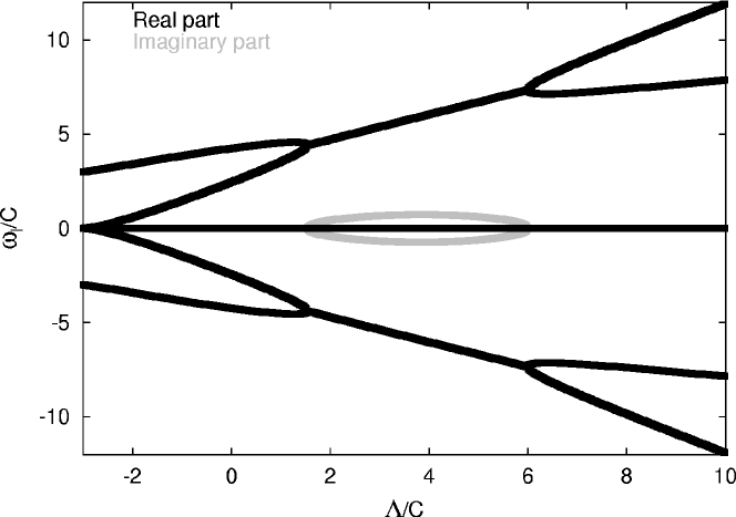
Figure 1: Scaled eigenfrequencies $\omega_{\rm l}/C$ of (8), (9) versus scaled frequency $\Lambda/C$ of the stationary solution (4). Dark (grey) lines represent real (imaginary) parts of $\omega_{\rm l}/C$.

These are real for small or large $\Lambda/C$, but complex for $x_{\ast}<\Lambda/C<6$ where $x_{\ast}\approx 1.5385$ is the only real solution to $x^{3}+6x^{2}+4x-24=0$ [23, 24] (figure 1.) Close to the linear limit $\Lambda/C\rightarrow-3$ we can expand (12) using $\lambda=A^{2}/C=\Lambda/C+3={\mathcal{N}}/2C$ as a small parameter, and obtain $|\omega_{\rm l+}|/C\approx 3+\lambda/3+4\lambda^{2}/27$ and $|\omega_{\rm l-}|/C\approx 2\lambda^{3/2}/3$. For $\omega_{\rm l+}$ the corresponding eigenmode can be expressed as

$$\left\{\left(\begin{array}[]{c}{a}_{n}\\ {b}_{n}\end{array}\right)\right\}=\left\{\left(\begin{array}[]{c}-2\lambda/9\\ 1+2\lambda/3\end{array}\right),\left(\begin{array}[]{c}-2\lambda/9\\ 1+2\lambda/3\end{array}\right),\left(\begin{array}[]{c}\lambda/9\\ 1\end{array}\right)\right\}+{\mathcal{O}}(\lambda^{2})$$ (13)

with ${\mathcal{K}}(\omega_{\rm l+})=-1$, while for $\omega_{\rm l-}$ the eigenmode is most conveniently described as

$$\left\{\left(\begin{array}[]{c}{U}_{n}\\ {W}_{n}\end{array}\right)\right\}=\left\{\left(\begin{array}[]{c}1\\ \sqrt{\lambda}\end{array}\right),\left(\begin{array}[]{c}1\\ \sqrt{\lambda}\end{array}\right),\left(\begin{array}[]{c}-2-2\lambda\\ -2\sqrt{\lambda}\end{array}\right)\right\}+{\mathcal{O}}(\lambda^{3/2})$$ (14)

with ${\mathcal{K}}(\omega_{\rm l-})=+1$. On the other hand, close to the anticontinuous limit $\Lambda/C\rightarrow\infty$, we obtain from (12) the eigenfrequencies $|\omega_{\rm l+}|/C\approx\Lambda/C+2$ and $|\omega_{\rm l-}|/C\approx 2\sqrt{\Lambda/C}+5\sqrt{C/\Lambda}$. Then, we can write the corresponding eigenmode for $\omega_{\rm l+}$ as

$$\left\{\left(\begin{array}[]{c}{a}_{n}\\ {b}_{n}\end{array}\right)\right\}=\left\{\left(\begin{array}[]{c}0\\ C/\Lambda\end{array}\right),\left(\begin{array}[]{c}0\\ C/\Lambda\end{array}\right),\left(\begin{array}[]{c}1\\ 0\end{array}\right)\right\}+{\mathcal{O}}((C/\Lambda)^{2})$$ (15)

with ${\mathcal{K}}(\omega_{\rm l+})=+1$, and the eigenmode corresponding to $\omega_{\rm l-}$ as

$$\left\{\left(\begin{array}[]{c}{U}_{n}\\ {W}_{n}\end{array}\right)\right\}=\left\{\left(\begin{array}[]{c}-\sqrt{C/\Lambda}\\ 1\end{array}\right),\left(\begin{array}[]{c}-\sqrt{C/\Lambda}\\ 1\end{array}\right),\left(\begin{array}[]{c}0\\ 2C/\Lambda\end{array}\right)\right\}+{\mathcal{O}}((C/\Lambda)^{3/2})$$ (16)

with ${\mathcal{K}}(\omega_{\rm l-})=-1$. Thus, the Krein signatures of the frequencies $\omega_{\rm l+}$ and $\omega_{\rm l-}$ are interchanged by the two Krein collisions at the boundaries of the complex regime, where the stationary solution is unstable (and the Krein signature undefined). Note also that the eigenmodes corresponding to nonzero $\omega_{\rm l}$ are symmetric around $n=3$, and thus their excitation breaks the spatial antisymmetry of the stationary solution around this site.

By considering the solution (4) as periodically repeated in an infinite lattice, it becomes, in the terminology of [4, 7, 8], a nonlinear standing wave with wave vector $Q=2\pi/3$ of ’type H’, for which (12) gives the subset of all eigenfrequencies corresponding to eigenmodes with spatial period 3. Close to the linear limit, (13) can then be interpreted as a phonon mode with wave vector $q=0$, while (14) represents a translational mode of wave vector $q=2\pi/3$ corresponding to a sliding towards the ’type E’ $Q=2\pi/3$ standing wave having a periodic repetition of the codes +1,-1,-1. Close to the anticontinuous limit, (15) represents a ’hole mode’ localized at the zero-amplitude site, while (16) corresponds to an internal oscillation at the non-zero amplitude sites. In the intermediate, unstable, regime, these characters of the eigenmodes become mixed.

3 Two-frequency solutions: bifurcations and linear stability

As shown in [14], exact, generally quasiperiodic, two-frequency solutions to the DNLS equation (1) exist and can be obtained from the ansatz

$$\psi_{n}(t)=\phi_{n}(t)\rme^{\rmi\omega_{0}t},$$ (17)

so that in the variables $\phi_{n}$ the DNLS equation (1) becomes

$$\rmi\dot{\phi}_{n}+C(\phi_{n+1}+\phi_{n-1}-2\phi_{n})+|\phi_{n}|^{2}\phi_{n}-\omega_{0}\phi_{n}=0.$$ (18)

Thus, the frequency $\omega_{0}$, corresponding to a pure phase rotation, becomes a parameter in (18), and for a given $\omega_{0}$ we may search for time-periodic solutions to (18) with frequency $\omega_{\rm b}$ fulfilling $\phi_{n}(t+2\pi/\omega_{\rm b})=\phi_{n}(t)$. In particular, any stationary solution to (1) of the form (3) is trivially a time-periodic solution to (18) of the form $\phi_{n}(t)=\phi_{n}^{(\Lambda)}\rme^{\rmi\omega_{\rm b}t}$ with frequency $\omega_{\rm b}=\Lambda-\omega_{0}$. However, when the linear eigenfrequencies $\omega_{\rm l}$ (12) are real and nonzero, in general (Lyapunov) families of genuine two-frequency solutions (generally quasiperiodic in the original frame) bifurcate from the stationary solutions when $\omega_{\rm l}(\Lambda)+\omega_{0}=\Lambda$. In the limit of small-amplitude oscillations around the stationary solution, these have frequencies $\omega_{\rm b}=\omega_{\rm l}$ in the frame rotating with the stationary frequency $\Lambda$, and coincide with the linear eigenmodes.

Using standard numerical continuation techniques described in [14], these two-frequency solutions can be continued versus $\omega_{\rm b}$ towards larger oscillation amplitudes away from the stationary solutions, and explicitly calculated to computer precision in their whole domain of existence. Using standard fortran routines for numerical integration and matrix inversion, when necessary in quadruple precision, we may generally obtain solutions fulfilling $||\phi_{n}(t+2\pi/\omega_{\rm b})-\phi_{n}(t)||<\epsilon$ with $\epsilon\sim 10^{-30}$, although for strongly unstable solutions inaccuracies in the numerical integration might limit the attainable precision to larger $\epsilon$. All results presented here have been obtained by first demanding a precision $\epsilon\sim 10^{-12}$, and then checked to be invariant when decreasing $\epsilon$.

The two-frequency solutions to (1) belong generally to two-parameter families, and there is some freedom in choosing independent parameters for the numerical continuation. (Since $C$ only yields a rescaling, we put $C=1$ in all numerical calculations.) One may choose e.g. frequencies $\omega_{0},\omega_{\rm b}$, or norm $\mathcal{N}$ and action (’area’) integral $I$ of the time-periodic solution to (18), i.e. in the frame rotating with frequency $\omega_{0}$. Using in this frame the canonical variables $\{\rmi\phi_{n}\},\{\phi_{n}^{\ast}\}$, corresponding to a transformation of the original Hamiltonian into $H^{\prime}=H+\omega_{0}{\mathcal{N}}$, $I$ becomes

$$I=\frac{1}{2\pi}\int_{0}^{2\pi/\omega_{\rm b}}\sum_{n=1}^{N}\phi_{n}^{\ast}\rmi\dot{\phi}_{n}\rmd t=H^{\prime}/\omega_{\rm b}-\frac{1}{4\pi}\int_{0}^{2\pi/\omega_{\rm b}}\sum_{n=1}^{N}|\phi_{n}|^{4}\rmd t.$$ (19)

For a stationary solution with $\rmi\dot{\phi}_{n}=-\omega_{\rm b}\phi_{n}$, $I$ is simply proportional to the norm ($I=-{\mathcal{N}}$), while for genuine two-frequency solutions $I$ and ${\mathcal{N}}$ are independent. In the following, we choose as independent parameters the frequency $\omega_{\rm b}$ in the rotating frame and the norm $\mathcal{N}$, and perform the continuation versus $\omega_{\rm b}$ for fixed norm by, at each value of $\omega_{\rm b}$, vary the parameter $\omega_{0}$ in (18) so to obtain a solution with the desired value of $\mathcal{N}$ (this procedure may fail at particular points if the dependence ${\mathcal{N}}(\omega_{0})$ for solutions at fixed $\omega_{\rm b}$ is nonmonotonous or multivalued; examples of this can be found below).

Linear stability of two-frequency solutions is obtained by linearizing (18) around an exact time-periodic $\phi_{n}(t)=\phi_{n}^{(\rm r)}(t)+\rmi\phi_{n}^{(\rm i)}(t)$ ($\phi_{n}^{(\rm r)}$, $\phi_{n}^{(\rm i)}$ real). The linearized equation for the small perturbation $\epsilon_{n}(t)$ will then have the same form as (7) with $\Lambda$ replaced by $\omega_{0}$, and the real and constant $\phi_{n}^{(\Lambda)}$ replaced by a generally complex and time-periodic $\phi_{n}(t)$. Decomposing $\epsilon_{n}(t)=\epsilon_{n}^{(\rm r)}(t)+\rmi\epsilon_{n}^{(\rm i)}(t)$ as in (10), the linearized equations can be written in Hamiltonian form as [23, 24]

$$\left(\begin{array}[]{c}\{\dot{\epsilon}_{n}^{(\rm r)}\}\\ \{\dot{\epsilon}_{n}^{(\rm i)}\}\end{array}\right)=\left(\begin{array}[]{cc}0&{\bf{1}}\\ {-\bf{1}}&0\end{array}\right)$$ (24)

$$\times\left(\begin{array}[]{cc}\left(\omega_{0}-3(\phi_{n}^{(\rm r)})^{2}-(\phi_{n}^{(\rm i)})^{2}\right){\bf 1}-C\Delta&-2\phi_{n}^{(\rm r)}\phi_{n}^{(\rm i)}{\bf{1}}\\ -2\phi_{n}^{(\rm r)}\phi_{n}^{(\rm i)}{\bf 1}&\left(\omega_{0}-(\phi_{n}^{(\rm r)})^{2}-3(\phi_{n}^{(\rm i)})^{2}\right){\bf 1}-C\Delta\end{array}\right)\left(\begin{array}[]{c}\{{\epsilon}_{n}^{(\rm r)}\}\\ \{{\epsilon}_{n}^{(\rm i)}\}\\ \end{array}\right)$$ (29)

(30)

where $\bf{1}$ denotes the $N$-dimensional unit matrix and $\Delta$ the discrete Laplacian, $\Delta\epsilon_{n}=\epsilon_{n+1}+\epsilon_{n-1}-2\epsilon_{n}$ (note that the second matrix in (30) is symmetric). Integrating (30) numerically over the period $T_{\rm b}=2\pi/\omega_{\rm b}$ of $\phi_{n}$ yields the symplectic $2N\times 2N$-dimensional Floquet matrix $\mathbf{F_{T_{\rm b}}}$ defined by

$$\left(\begin{array}[]{c}\{\epsilon_{n}^{(\rm r)}(T_{\rm b})\}\\ \{\epsilon_{n}^{(\rm i)}(T_{\rm b})\}\end{array}\right)=\mathbf{F_{T_{\rm b}}}\left(\begin{array}[]{c}\{\epsilon_{n}^{(\rm r)}(0)\}\\ \{\epsilon_{n}^{(\rm i)}(0)\}\end{array}\right),$$ (31)

and the solution $\phi_{n}(t)$ is linearly stable if and only if all eigenvalues $\alpha$ of $\mathbf{F_{T_{\rm b}}}$ lie on the unit circle. In the particular case of a stationary solution, the eigenvalues $\alpha$ of $\mathbf{F_{T_{\rm b}}}$ are related to the linear eigenfrequencies $\omega_{\rm l}$ of (8), (9) as $\alpha=\rme^{\rmi 2\pi\omega_{\rm l}/\omega_{\rm b}}$ with $\omega_{\rm b}=\Lambda-\omega_{0}$.

For a genuine two-frequency solution there are two arbitrary phases, one corresponding to global phase rotations which is put to zero at $t=0$ in the ansatz (17), and another corresponding to the phase of the time-periodic solution in the rotating frame which we fix by imposing time reversibility, $\phi_{n}^{\ast}(-t)=\phi_{n}(t)$ (i.e. $\phi_{n}^{(\rm i)}(0)=0$). To each of these phase degeneracies there is a corresponding solution to the linearized equations (30) with period $T_{\rm b}$, and thus a pair of eigenvalues $\alpha=+1$ of $\mathbf{F_{T_{\rm b}}}$ [14]. The solution corresponding to an infinitesimal global phase rotation is $\epsilon_{n}(t)=\rmi\phi_{n}(t)$ (i.e. $\left(\{\epsilon_{n}^{(\rm r)}\},\{\epsilon_{n}^{(\rm i)}\}\right)=\left(\{-\phi_{n}^{(\rm i)}\},\{\phi_{n}^{(\rm r)}\}\right)$), while the solution corresponding to an infinitesimal translation of the phase in the rotating frame is $\epsilon_{n}(t)=\dot{\phi}_{n}(t)$ (i.e. $\left(\{\epsilon_{n}^{(\rm r)}\},\{\epsilon_{n}^{(\rm i)}\}\right)=\left(\{\dot{\phi}_{n}^{(\rm r)}\},\{\dot{\phi}_{n}^{(\rm i)}\}\right)$). (Note that for stationary solutions, these become linearly dependent and there is only one pair of eigenvalues at +1.) Thus, for the particular case $N=3$ there is for a genuine two-frequency solution at most one pair of Floquet eigenvalues $\alpha$ not identical to +1, so the only way such a solution can change its stability is through collisions of the members of this pair either at +1 or at -1.

Furthermore, due to the invariance of the DNLS equation and its linearization under the transformation $\phi_{n}\rightarrow-\phi_{n}$ and the antisymmetry ($\phi_{2}^{(\Lambda)}=-\phi_{1}^{(\Lambda)};\phi_{3}^{(\Lambda)}=0$) of the particular stationary solutions, the families of two-frequency solutions bifurcating from them will have the additional space-time symmetry $\phi_{1}(t+T_{\rm b}/2)=\phi_{2}(t),\phi_{3}(t+T_{\rm b}/2)=\phi_{3}(t)$. This implies that the time-periodic solution $\phi_{n}$ with $\phi_{1}(0)\neq\phi_{2}(0)$ contains only odd harmonics of its fundamental frequency $\omega_{\rm b}$. As a conseqeunce, collisions of Floquet eigenvalues at -1 corresponding to period-doubling bifurcations will not yield instabilities, which can be seen by decomposing the Floquet matrix as $\mathbf{F_{T_{\rm b}}}={\mathbf{P}_{1\leftrightarrow 2}}\mathbf{F_{T_{\rm b}/2}}{\mathbf{P}_{1\leftrightarrow 2}}\mathbf{F_{T_{\rm b}/2}}$, where $\mathbf{F_{T_{\rm b}/2}}$ is the matrix obtained by integrating (30) over half a period and ${\mathbf{P}_{1\leftrightarrow 2}}$ interchanges sites 1 and 2. Thus, only collisions of eigenvalues $\beta$ to ${\mathbf{P}_{1\leftrightarrow 2}}\mathbf{F_{T_{\rm b}/2}}$ at $\beta=\pm 1$ can yield instabilities, and they must all correspond to eigenvalue collisions at $\alpha=+1$ for the total Floquet matrix $\mathbf{F_{T_{\rm b}}}$ since $\alpha=\beta^{2}$. Below, we report the numerical stability properties in terms of eigenvalues $\beta$ rather than $\alpha$.

3.1 The low-amplitude ’Type I’ bifurcation

3.1.1 Small ${\mathcal{N}}/C$.

We first discuss some properties of the two families of two-frequency solutions bifurcating from the stationary solution for $\Lambda/C<x_{\ast}$, i.e. ${\mathcal{N}}/C<9.077...$, corresponding to the linear modes with asymptotic oscillation patterns (13) and (14), respectively, for small ${\mathcal{N}}/C$. Their continuation versus $\omega_{\rm b}$ for fixed ${\mathcal{N}}/C=5$ is illustrated in figure 2.

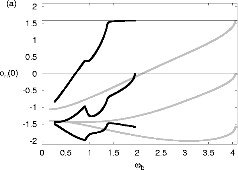
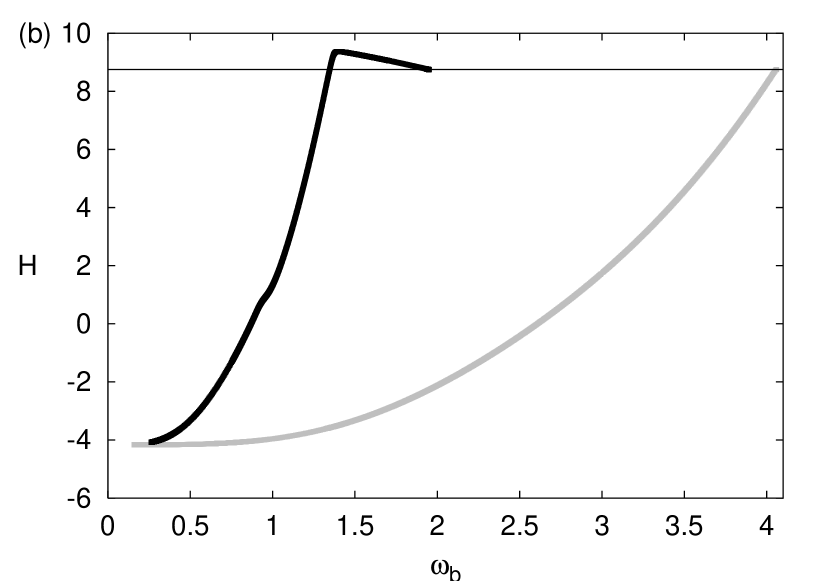
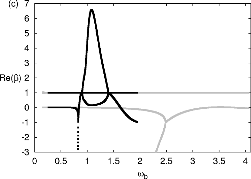
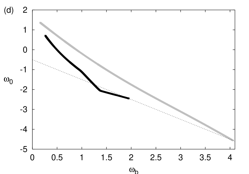
Figure 2: Continuation versus $\omega_{\rm b}$ at fixed norm ${\mathcal{N}}=5$ ($C=1$) of the two-frequency solutions bifurcating from the stationary solution (4) with $\Lambda=-0.5$ at $\omega_{\rm b}=\omega_{\rm l\pm}$ given by (12); black [grey] curves correspond to $\omega_{\rm l-}$ [$\omega_{\rm l+}$]. (a) Initial amplitudes $\phi_{n}(0)$ for $n=1$ (upper), $n=2$ (lower) and $n=3$ (middle curves); (b) Hamiltonian $H$ (2); (c) real parts of stability eigenvalues $\beta$; (d) frequency $\omega_{0}$ of the rotating frame. The horizontal lines in (a) and (b) and the dashed line in (d) correspond to the stationary solution according to (4) and (6). The large negative eigenvalues not shown in (c) for small $\omega_{\rm b}$ will continue to decrease rapidly (e.g. at $\omega_{\rm b}=0.2$, $\beta\approx-10^{9}$ for the grey solution). For $\omega_{b}\lesssim 0.90$, the black solution is identical to the grey at frequency $3\omega_{b}$.

For both solutions, the continuation from the stationary solution is monotonous in the direction of decreasing $\omega_{\rm b}$, and they are linearly stable for a rather large interval of frequencies $\omega_{\rm b}\leq\omega_{\rm l\pm}$, but become strongly unstable at small $\omega_{\rm b}$ (figure 2 (c)). For the (grey) solution corresponding to $\omega_{\rm l+}$, the instability is caused by a collision of eigenvalues $\beta$ at -1 producing a rapid and monotonous growth of $|\beta|$ for small $\omega_{\rm b}$. This behaviour is typical for ${\mathcal{N}}/C>4.5$. For ${\mathcal{N}}/C<4.5$, $\beta$ attains a minimum value and then returns towards the unit circle, and finally through a collision at $\beta=-1$ the grey solution bifurcates into the homogeneous stationary solution with $\phi_{1}=\phi_{2}=\phi_{3}=-\sqrt{{\mathcal{N}}/3}$, which is linearly stable in this regime [23, 24]. (The continuation versus $\omega_{b}$ is typically non-monotonous close to this bifurcation point.) At ${\mathcal{N}}/C=4.5$ the homogeneous solution becomes unstable [23], and by analyzing the dynamics of the grey solution in the limit $\omega_{\rm b}\rightarrow 0$ for ${\mathcal{N}}/C>4.5$, we find that it asymptotically approaches a (strongly unstable) solution consisting of homoclinic connections of unstable and stable manifolds of the homogeneous solution (as further discussed in section 3.1.3, see also figure 9 (b) below).

The scenario for the (black) solution corresponding to $\omega_{\rm l-}$ is more complicated: it first becomes unstable through an eigenvalue collision at $\beta=+1$, associated with a change of nature of the solution as seen in figure 2 (a). This is related to a third-harmonic resonance with the grey solution, and the instability appears at $\omega_{\rm b}$ close to (but not exactly at) $\omega_{\rm l+}/3$. The instability first grows when decreasing $\omega_{\rm b}$, but attains a maximum and finally, through a second collision at $+1$, the black solution becomes identical to the (stable) grey solution at frequency $3\omega_{\rm b}$, which becomes unstable slightly after. As mentioned above, for symmetry reasons higher-harmonic resonances can occur only for odd harmonics. Since $\omega_{\rm l-}$ decreases towards zero when ${\mathcal{N}}/C$ decreases while $\omega_{\rm l+}$ remains finite, for smaller ${\mathcal{N}}/C$ the resonances are of higher order. Thus, for example when ${\mathcal{N}}/C$ approaches from above a critical value $\sim 3.53$ (where $\omega_{\rm l+}=3\omega_{\rm l-}$) the value of $\omega_{\rm b}$ where the black solution becomes unstable approaches the linear frequency $\omega_{\rm b}=\omega_{\rm l-}$, and for smaller ${\mathcal{N}}/C$ the third-harmonic resonance disappears and the solution is stable until a similar fifth-harmonic resonance appears for smaller $\omega_{\rm b}$. It is interesting to note, that if the numerical continuation is performed ’carelessly’, i.e. with larger steps, one might ’jump’ the regime yielding a $p$th harmonic resonance and catch instead a solution in apparent (but non-smooth!) continuation of the original solution, as if the resonance had not existed. This solution can then be continued towards smaller $\omega_{\rm b}$ until a ($p+2$)th harmonic resonance is encountered, etc. Thus, a cascade of higher-order resonances will result, and the scenario is analogous to that previously found for higher-order resonances in Klein-Gordon chains in [7] (e.g. figures 12 and 16 in this paper) and [60]. The behaviour shown in figure 2 is typical for $3.6\lesssim{\mathcal{N}}/C\lesssim 5.5$, while for ${\mathcal{N}}/C\approx 5.6$ two additional eigenvalue collisions at $\beta=+1$, producing a new pair of small stability/instability regimes, appear slightly before the transformation of the black solution into the grey $3\omega_{\rm b}$-solution. A further increase of ${\mathcal{N}}/C$ yields one more pair of small regimes of stability/instability through a collision at $\beta=-1$, and for ${\mathcal{N}}/C\gtrsim 6.8$ the continuation versus $\omega_{\rm b}$ becomes nonmonotonous of ’Z-type’, where three different solutions of the family have the same frequency $\omega_{\rm b}$, in some regime before the final bifurcation with the $3\omega_{b}$-solution (similar behaviour was also observed in [7, 60]).

Note also (figure 2 (b)) that the Hamiltonian of the black solution changes slope so that ${\rm d}H/{\rm d}\omega_{\rm b}=0$ at the first eigenvalue collision at $\beta=+1$ (but not at the second where the solution transforms to the grey third-harmonic solution). Moreover, the additional eigenvalue collisions at $\beta=+1$ for ${\mathcal{N}}/C\approx 5.6$ also produce a new pair of local min/max for $H(\omega_{\rm b})$ at the collision points. Generally (see also several similar examples below), it appears that ${\rm d}H/{\rm d}\omega_{\rm b}=0$ for two-frequency solutions at fixed norm could be a sufficient (but not necessary) condition for a change in stability through an eigenvalue collision at +1, analogous to the wellknown criteria ${\rm d}{\mathcal{N}}/{\rm d}\Lambda=0$ for stationary solutions [58] and the more general ${\rm d}{\mathcal{I}}/{\rm d}\omega=0$ for periodic solutions of Hamiltonian systems with frequency $\omega$ and action ${\mathcal{I}}$ [28]. Indeed, this could be expected since a turning point of $H$ for relative periodic solutions at fixed $\mathcal{N}$ should correspond to a saddle-centre bifurcation.

3.1.2 Around the bifurcation point.

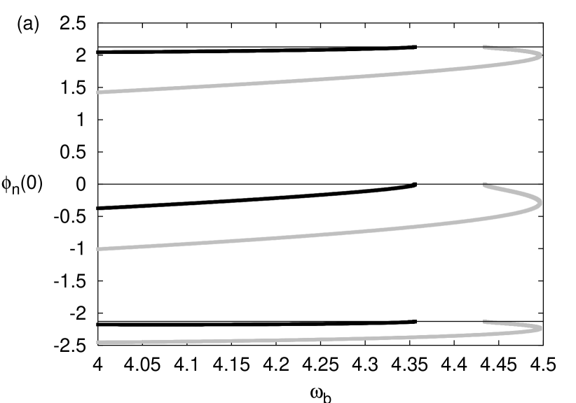
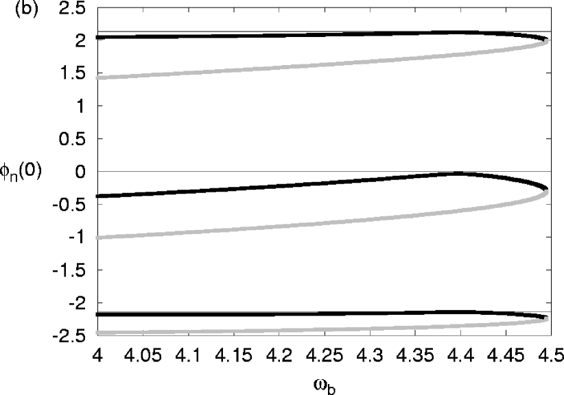
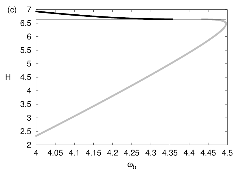
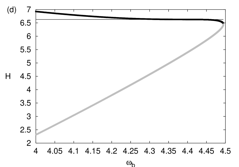
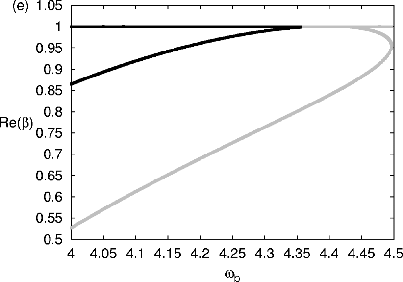
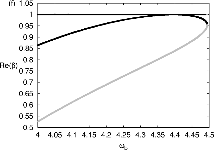
Figure 3: Same as figure 2 (a)-(c) but for ${\mathcal{N}}=9.07$ (left figures) and ${\mathcal{N}}=9.08$ (right figures). In (a), (c), (e) the meaning of the black and grey curves is the same as in figure 2, while in (b), (d), (f) they illustrate the two different but connected branches of coexisting two-frequency solutions continued from the solutions in the left figures.

Focusing on the regime of $\omega_{\rm b}$ close to $\omega_{\rm l\pm}$, we compare the solutions on both sides of the bifurcation point ${\mathcal{N}}/C\approx 9.077$ in figure 3. For $8.95\lesssim{\mathcal{N}}/C\lesssim 9.077$, the continuation of the grey solution from the stationary solution is no longer monotonous versus $\omega_{\rm b}$, but goes first in the direction of increasing $\omega_{\rm b}$ from $\omega_{\rm l+}$ up to a maximum value, and then turns and continues towards smaller $\omega_{\rm b}$ similarly as in figure 2. As mentioned above, this multivaluedness causes numerical problems for the method of continuing for fixed norm by varying $\omega_{0}$ at one point (close to but different from the turning point), where ${\rm d}{\mathcal{N}}/{\rm d}\omega_{0}$ for fixed $\omega_{\rm b}$ becomes infinite.

At the bifurcation point ${\mathcal{N}}/C\approx 9.077$ the gap separating the black and grey families of solutions in figure 3 (a), (c), (e) closes (since $\omega_{\rm l-}=\omega_{\rm l+}$ at this point), and for larger ${\mathcal{N}}/C$ as in figure 3 (b), (d), (f) they constitute two connected branches of a single family of two-frequency solutions, now separated from the stationary solution. Note that even though the two-frequency solutions are detached from the stationary solution on the superthreshold side of the bifurcation (where the latter is unstable and $\omega_{\rm l\pm}$ are complex), the distance between the two-frequency family and the stationary solution (which can be expressed in some suitable norm) decreases continuously to zero when approaching the bifurcation point from above. This is the characteristic property of a type I HH bifurcation [30], and the scenario in figure 3 is equivalent to that of figure 2 in [30] (see also figure 2(b) in [27], [28]). The importance of this property for the dynamics of the unstable stationary solution will be illustrated in section 4.

3.1.3 Larger ${\mathcal{N}}/C$.

Increasing ${\mathcal{N}}/C$ on the superthreshold side of the type I bifurcation, the continued solutions persist as two connected branches of a single family detached from the stationary solution (4), continuously increasing the distance to it. The typical behaviour for larger ${\mathcal{N}}/C$ is illustrated in figure 4.

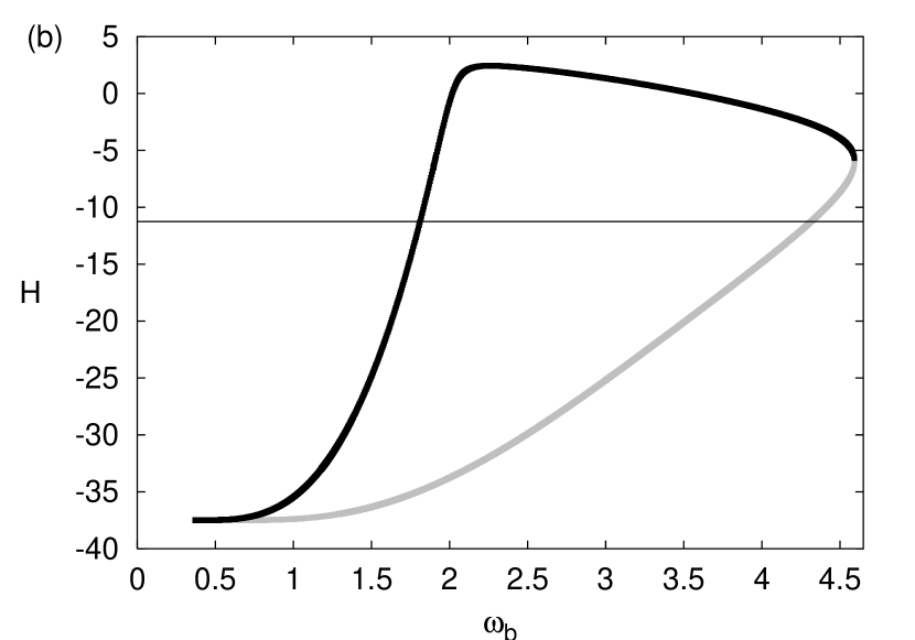
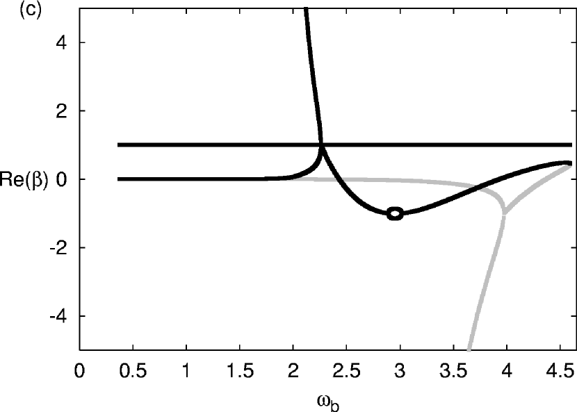
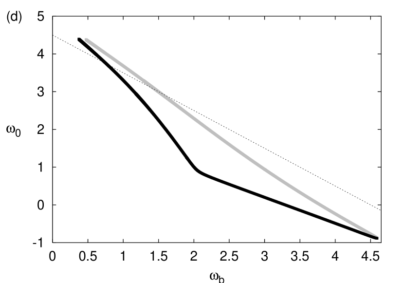
Figure 4: Continuation versus $\omega_{\rm b}$ at fixed norm ${\mathcal{N}}=15$ of the two-frequency solutions continued from those of figures 2-3. The meaning of the black and grey parts is the same as in figure 3 (b), (d), (f); other quantities have the same meaning as in figure 2. The eigenvalues not shown in (c) for small $\omega_{\rm b}$ continue to decrease [increase] monotonously for the grey [black] solution; $\beta\approx-10^{12}$ [$\beta\approx 10^{11}$] at $\omega_{\rm b}=0.5$.

Compared to the earlier discussed examples we note two main differences. First, there is a small bubble of instability through a collision at $\beta=-1$ for the black solution in figure 4 (c) for $\omega_{\rm b}\approx 2.9-3.0$. In fact, such an instability occurs in many regimes also for smaller ${\mathcal{N}}/C$ (e.g. for ${\mathcal{N}}/C\gtrsim 5$), but it is then very weak and practically invisible numerically, while it grows considerably stronger for larger ${\mathcal{N}}/C$. Second, for ${\mathcal{N}}/C\gtrsim 9.45$ the black solution no longer transforms into the third-harmonic of the grey solution for small $\omega_{\rm b}$, but approaches as $\omega_{\rm b}\rightarrow 0$ a (strongly unstable) solution with the same values of $\phi_{n}(0)$, $H$ and $\omega_{0}$ as the asymptotic grey solution (figure 4 (a), (b), (d)), but with $\beta\rightarrow+\infty$ (figure 4 (c)). Thus, these asymptotic solutions are not identical, although they both consist of homoclinic connections of the unstable homogeneous stationary solution $\phi_{1}=\phi_{2}=\phi_{3}$ (which has a doubly degenerate unstable eigenvalue [23] so the corresponding stable and unstable manifolds can be connected in different ways). Analysis of the dynamics yields that the grey solution in half a period contains two stable and two unstable manifolds from the homogeneous solution, and they are all associated with two-site localization with a third site of small $|\phi_{n}|^{2}$ as for $t=0$ in figure 4 (a) (see figure 9 (b) below). The black solution on the other hand contains three stable and three unstable manifolds in one half-period, and of these two pairs are associated with one-site localization with two sites of smaller $|\phi_{n}|^{2}$, and only one pair with two-site localization (see figure 9 (a)).

We also note, by comparing figures 3 (d) and 4 (b), that while close to the bifurcation point the Hamiltonian for the unstable stationary solution (6) cuts the two-frequency solution family on the black branch (figure 3 (d)), the corresponding intersection point appears for larger ${\mathcal{N}}/C$ on the grey branch (figure 4 (b)). This change of branch occurs at ${\mathcal{N}}/C\approx 10.6$, which, as will be discussed in section 4 below, is the value where the self-trapping transition of the unstable stationary solution is observed.

3.2 The high-amplitude ’Type II’ bifurcation

Turning our attention to the two-frequency solutions associated with the high-amplitude Krein collision for the stationary solution at $\Lambda/C=6$, i.e. ${\mathcal{N}}/C=18$, we first describe some properties of these solutions (which are not identical to those involved in the low-amplitude bifurcation) on the stable side, i.e. for ${\mathcal{N}}/C>18$.

3.2.1 Large ${\mathcal{N}}/C$.

The continuation of the two-frequency solutions corresponding to linear modes with asymptotic oscillation patterns (15) and (16), respectively, for large ${\mathcal{N}}/C$, is shown in figure 5 for ${\mathcal{N}}/C=20$.

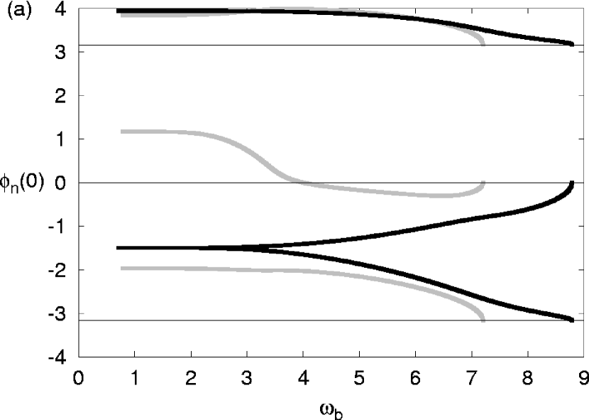
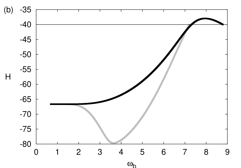
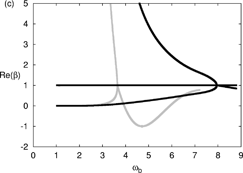
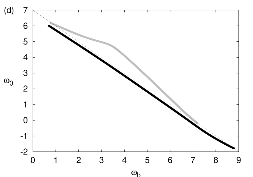
Figure 5: Same as figure 2 but for the two-frequency solutions bifurcating from the stationary solution with $\Lambda=7$ at ${\mathcal{N}}=20$; grey [black] curves corresponding to solutions bifurcating at $\omega_{\rm b}=\omega_{\rm l-}$ [$\omega_{\rm b}=\omega_{\rm l+}$]. The eigenvalues not shown in (c) for small $\omega_{\rm b}$ increase monotonously for both solutions ($\beta\sim 10^{8}$ at $\omega_{\rm b}=0.8$).

For both solutions the continuation from the linear modes is monotonous in the direction of decreasing $\omega_{\rm b}$, and they are linearly stable in some regime $\omega_{\rm b}<\omega_{\rm l\pm}$ but become strongly unstable for smaller $\omega_{\rm b}$ (figure 5 (c)). The stability regime for the black solution is rather small, and it is unstable in the whole range where also the grey solution exists. Also here (figure 5 (b)) ${\rm d}H/{\rm d}\omega_{\rm b}=0$ at the instability thresholds occurring through collisions at $\beta=+1$ (there is also a tiny instability for the grey solution caused by collisions at $\beta=-1$ for $\omega_{\rm b}\approx 4.70-4.73$). As $\omega_{\rm b}\rightarrow 0$ also these solutions approach homoclinic connections of stable and unstable manifolds of the homogeneous stationary solution $\phi_{1}=\phi_{2}=\phi_{3}$, which however are distinct both from each other and from those described in section 3.1. They both contain one stable and one unstable manifold in each half-period, but while for the black solution the dynamics is of one-site-localization type with two sites of small equal $|\phi_{n}|^{2}$ (figure 9 (c) below), the dynamics of the grey solution have all three sites of unequal amplitude as seen in figure 5 (a) (see figure 9 (d)).

3.2.2 Around the bifurcation point.

Approaching from above the bifurcation point ${\mathcal{N}}/C=18$ the frequencies $\omega_{\rm l+}$ and $\omega_{\rm l-}$ approach each other, as do the corresponding families of two-frequency solutions which at ${\mathcal{N}}/C\approx 18.7$ coincide at $\omega_{\rm b}\approx 6.8$ ($<\omega_{\rm l-}\approx 7.1$). At this point they bifurcate with each other, and compared to the scenario in figure 5 (c) an additional simultaneous collision at $\beta=+1$ appears for both solutions, in the regime where for larger ${\mathcal{N}}/C$ the black solution was unstable and the grey stable. For smaller ${\mathcal{N}}/C$ the solutions split into a low-frequency and a high-frequency part separated by a forbidden gap in $\omega_{\rm b}$ as illustrated by figure 6.

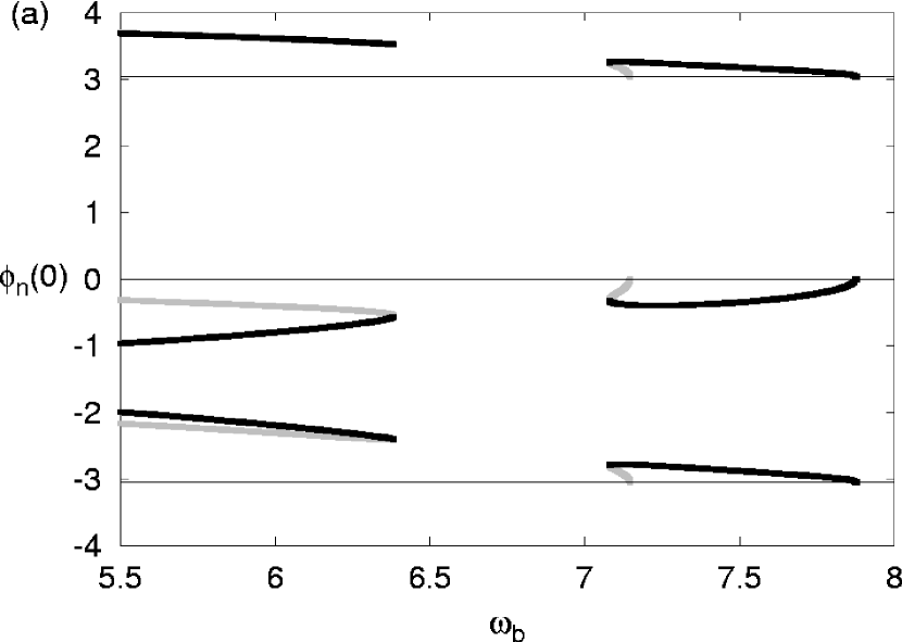
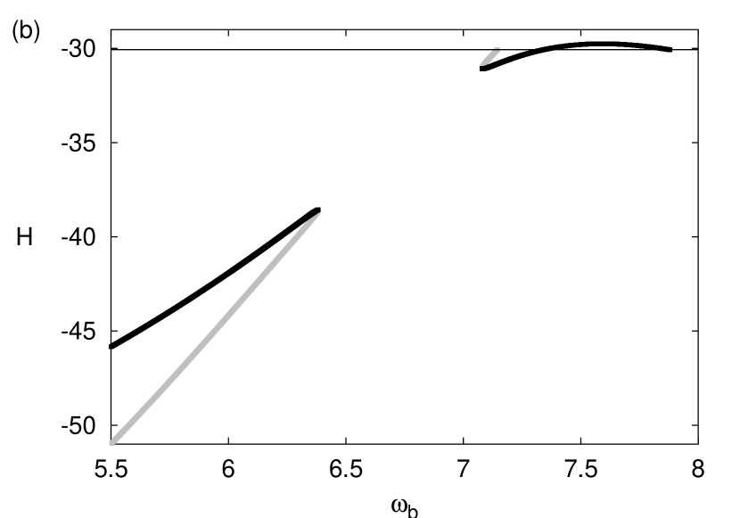
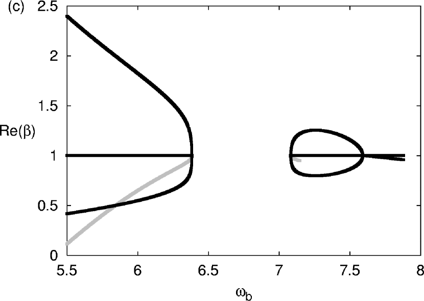
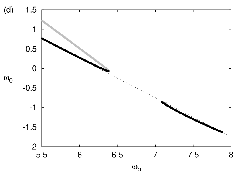
Figure 6: Continuation of the solutions in figure 5 for ${\mathcal{N}}=18.5$. The behaviour for $\omega_{\rm b}<5.5$ is qualitatively the same as in figure 5.

Thus, only the high-frequency part is now connected to the stationary solution.

Decreasing further ${\mathcal{N}}/C$ the high-frequency part shrinks as $\omega_{\rm l+}$ and $\omega_{\rm l-}$ approach each other, and furthermore at ${\mathcal{N}}/C\approx 18.2$ (figure 7 (a), (c), (e)) the continuation of the grey solution from $\omega_{\rm b}=\omega_{\rm l-}$ changes direction to occur towards larger $\omega_{\rm b}$.

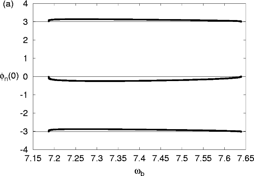
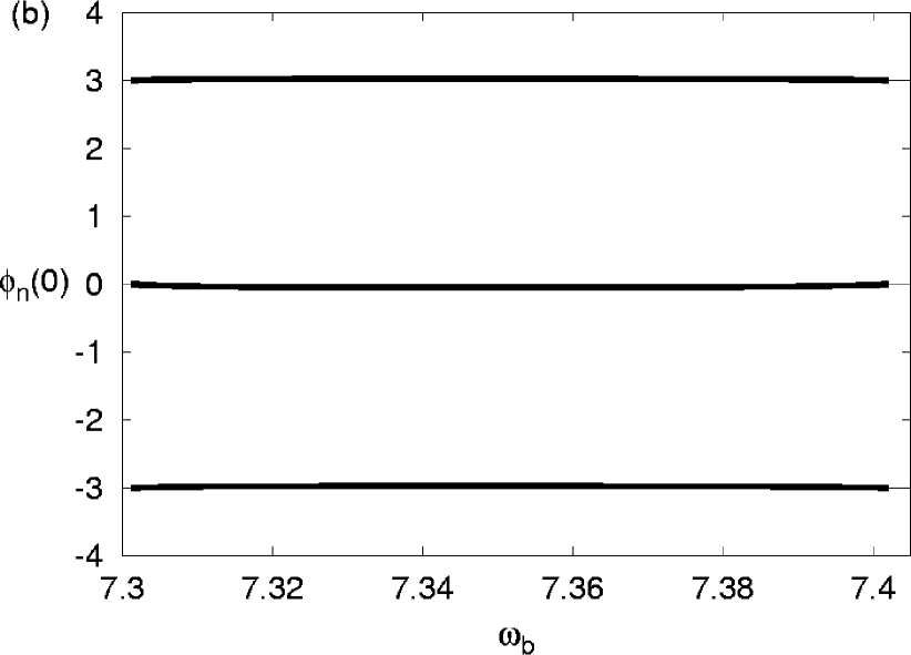
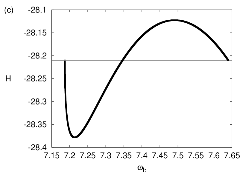
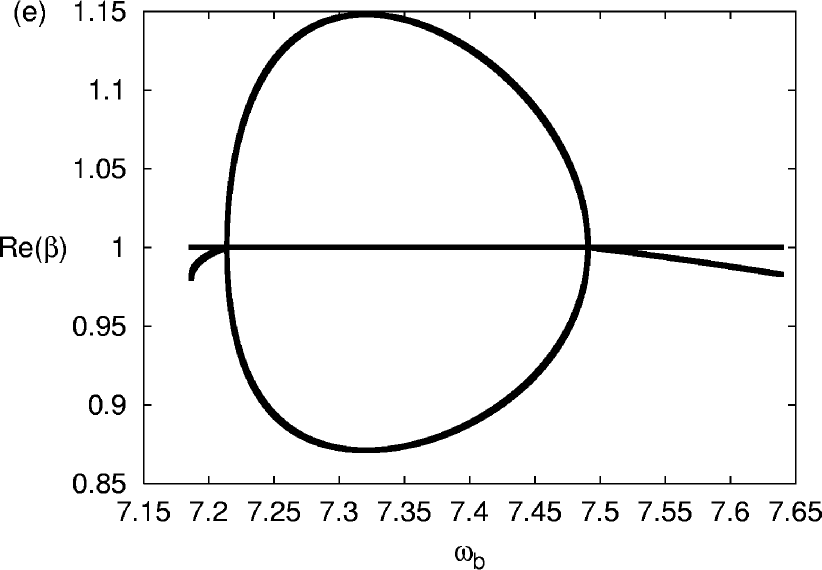
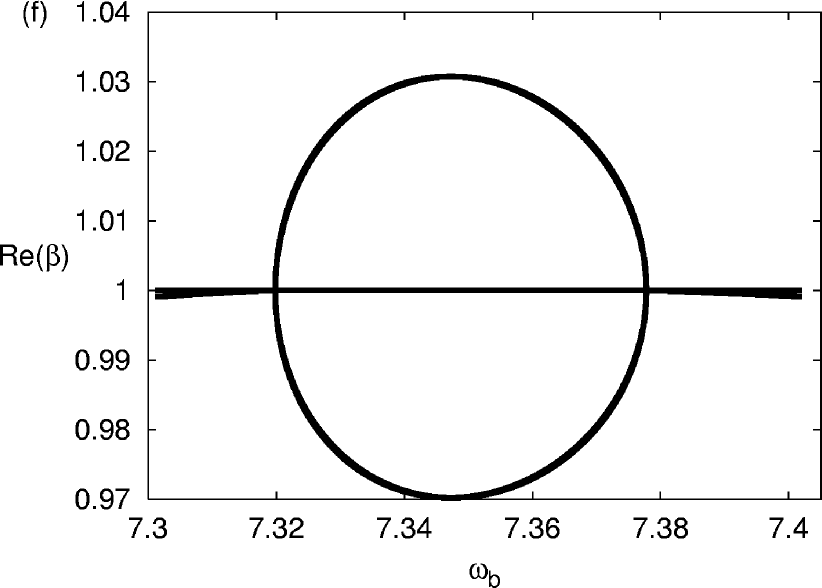
Figure 7: Continuation of the high-frequency branches of figure 6 (a)-(c) for ${\mathcal{N}}=18.2$ (left figures) and ${\mathcal{N}}=18.01$ (right figures). At ${\mathcal{N}}=18.2$ there is still a tiny remainder of the grey part of previous figures which continues approximately $10^{-6}$ in the direction of negative $\omega_{\rm b}$ from the linear value $\omega_{\rm b}=\omega_{\rm l-}\approx 7.186\,6898$.

Thus, for $18<{\mathcal{N}}/C\lesssim 18.2$ the high-frequency branch consists of one single family which through a monotonous continuation versus $\omega_{\rm b}$ connects the linear eigenmode at $\omega_{\rm l-}$ with that at $\omega_{\rm l+}$ (figure 7 (b), (d), (f)). The solutions are linearly stable close to $\omega_{\rm b}=\omega_{\rm l\pm}$ but unstable for intermediate frequencies (figure 7 (f)) (note also the ’inverse N-shape’ of $H(\omega_{\rm b})$ in figure 7 (d) consistent with the negative Krein signature of $\omega_{\rm l-}$ and the positive of $\omega_{\rm l+}$). At the bifurcation point ${\mathcal{N}}/C=18$, $\omega_{\rm l-}=\omega_{\rm l+}$ and the loop of surrounding two-frequency solutions shrinks to zero. Consequently, for ${\mathcal{N}}/C<18$ where the stationary solution is unstable, no nearby two-frequency solutions exist, and the scenario is that of a type II HH bifurcation [30] (cf. figure 3 in [30] and figure 2(a) in [27], [28]). However, the low-frequency branches in figure 6 exist also for ${\mathcal{N}}/C<18$, but at a considerable distance from the stationary solution (e.g. at ${\mathcal{N}}=18$ and $C=1$ the Hamiltonian (6) for the stationary solution is $H=-27$, while its maximum value on the disconnected branch of two-frequency solutions is $H\approx-39.4$). We illustrate the consequences for the dynamics of the unstable stationary solution in section 4.

3.2.3 Smaller ${\mathcal{N}}/C$.

Continuing the low-frequency branches of figure 6 towards smaller ${\mathcal{N}}/C$, their features remain qualitatively the same. The example for ${\mathcal{N}}/C=15$ in figure 8 shows that they are distinct from those originating from the low-amplitude bifurcation (cf. figure 4).

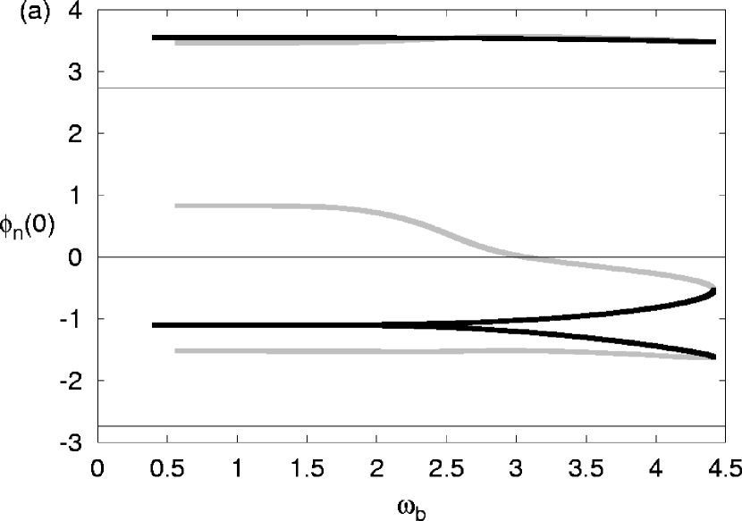
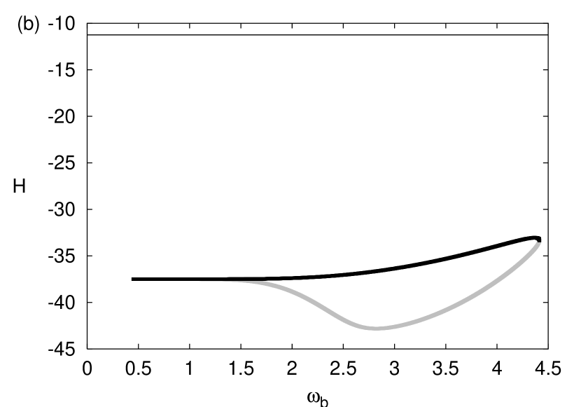
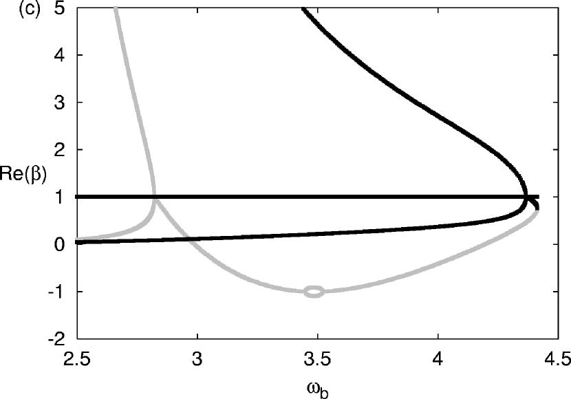
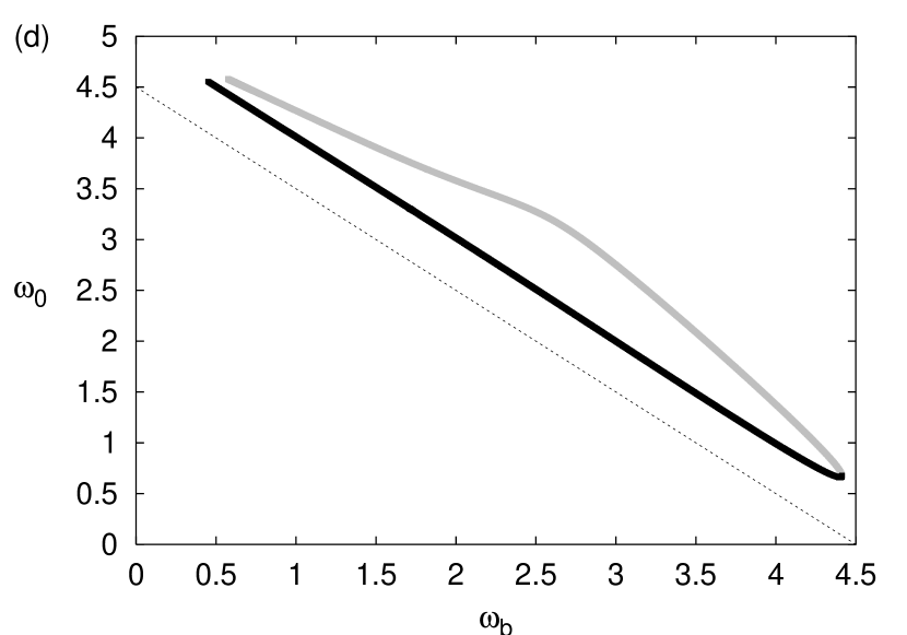
Figure 8: Continuation of the low-frequency branches of figure 6 for ${\mathcal{N}}=15$. The eigenvalues not shown in (c) for small $\omega_{\rm b}$ increase monotonously for both solutions ($\beta\sim 5\cdot 10^{6}$ at $\omega_{\rm b}=0.8$). As before, horizontal lines in (a), (b) and dashed line in (d) show corresponding quantities for the (unstable) stationary solution (4) ($C=1$).

Moreover, they remain at a large distance from the unstable stationary solution (4) also when ${\mathcal{N}}/C$ decreases (see e.g. the large difference in $H$ in figure 8 (b)), and their maximum value of $\omega_{\rm b}$ (i.e. where the black and grey branches meet) continues to decrease (e.g. at ${\mathcal{N}}=10$ and $C=1$ they meet at $\omega_{\rm b}\approx 2.33$).

To illustrate the different nature of the solutions in figures 4 and 8 for small $\omega_{\rm b}$, we plot in figure 9 the resulting dynamics for one half-period $T_{\rm b}/2$ (remembering that $\phi_{1}(t+T_{\rm b}/2)=\phi_{2}(t),\phi_{3}(t+T_{\rm b}/2)=\phi_{3}(t)$ yields the complete dynamics) at $\omega_{\rm b}=0.58$.

Figure 9: Dynamics for one half-period of the four different solutions in figures 4 and 8 at ${\mathcal{N}}=15$, $\omega_{\rm b}=0.58$ and $C=1$. (a) and (c) [(b) and (d)] correspond to the black [grey] solutions in figures 4 and 8, respectively.

As $\omega_{\rm b}$ decreases the flat parts of the curves will flatten and stretch out in time, so that as $\omega_{\rm b}\rightarrow 0$ the previously described asymptotic solutions are approached. (Since these solutions are strongly unstable, their accurate numerical determination even at $\omega_{\rm b}=0.58$ and for only half a period requires working in quadruple precision.)

4 Instability-generated dynamics

Let us now discuss the dynamics resulting from initial conditions taken as a slightly perturbed stationary solution (4) in various parts of its Krein instability regime, with three examples shown in figure 10.

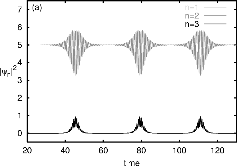
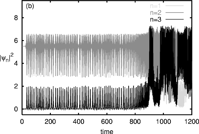
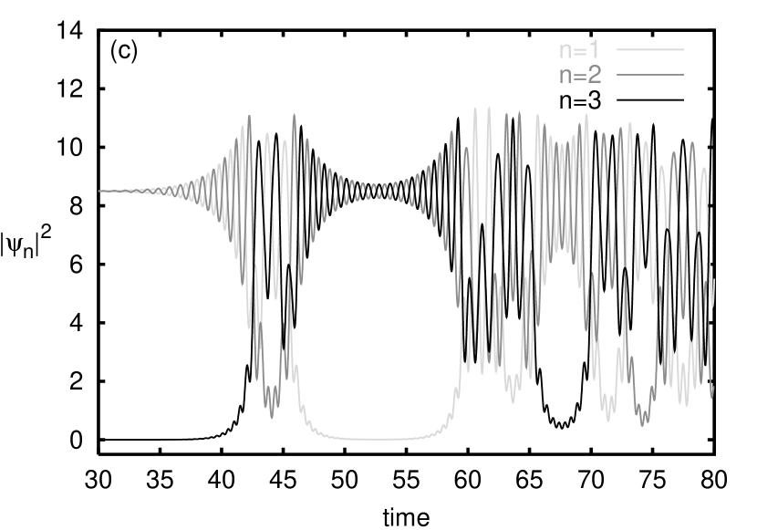
Figure 10: Typical instability-generated dynamics for randomly perturbed unstable stationary solutions (4) with $C=1$ and (a) ${\mathcal{N}}=10$, (b) ${\mathcal{N}}=11$, and (c) ${\mathcal{N}}=17$, respectively. The size of the initial perturbation is of the order of $10^{-8}$.

Close to the low-amplitude instability threshold (figure 10 (a)), the dynamics remains trapped forever in a state of bounded oscillations around the initial solution. In particular, the amplitude of the initially unexcited site ($n=3$) always remains small compared to the other two sites. As ${\mathcal{N}}/C$ increases the amplitude of these oscillations increases, and above a certain value ${\mathcal{N}}/C\approx 10.6$ the self-trapping is destroyed and the dynamics of all three sites becomes qualitatively the same. Slightly above this value the dynamics is still initially trapped (figure 10 (b)), but finally the trapping is destroyed and the amplitude of the third site increases drastically. The length of the initial transient approaches infinity as ${\mathcal{N}}/C\rightarrow\sim 10.6$, but decreases for increasing ${\mathcal{N}}/C$ so that close to the high-amplitude instability threshold ${\mathcal{N}}/C=18$ no transient is observed (figure 10 (c)). In all cases, the dynamics in the untrapped regime can be characterized as ’intermittent population inversion’, which was observed also for certain initial conditions of the (nonequivalent) trimer studied in [53]. This is most clearly seen in figure 10 (c). Here, one can during certain time intervals unambiguously identify two sites of large amplitude and a single small-amplitude site, which changes from initially being $n=3$ to $n=2$, and then, during a rather long time, to $n=1$. After that follows a regime of more complicated oscillations, which then again is followed by a regime with a single small-amplitude site changing from $n=3$ to $n=1$, etc.

To understand more clearly the origin of this self-trapping transition, we analyze the dynamics close to the unstable stationary solution in terms of Poincaré sections. They can be introduced in many different ways; here we apply similar ideas as in [35] making use of the transformation into action-angle variables $\{P_{n},\theta_{n}\}$ defined by $\psi_{n}=\sqrt{P_{n}}\rme^{-\rmi\theta_{n}}$ (a slightly different approach was used in [53]). It is then convenient to replace one of the action variables, which we here choose as $P_{1}$, with the conserved quantity ${\mathcal{N}}$. Then, the angle-variables conjugated to the set of generalized momenta $\{{\mathcal{N}},P_{2},P_{3}\}$ are [35] $\{\theta_{1},\theta_{2}-\theta_{1},\theta_{3}-\theta_{1}\}$, so that $\theta_{1}$ describing an overall phase becomes an ignorable coordinate. Thus, the essential dynamics takes place in a four-dimensional space where the surface of constant energy $H$ is three-dimensional, so that a proper Poincaré section through it becomes two-dimensional. Consequently, although chaotic trajectories may fill a large portion of the available phase space [24, 35], Arnold diffusion is prohibited [34, 61] since the presence of any regular KAM tori will disconnect the phase space. (Arnold diffusion does however appear for the four-site DNLS model [61, 62].)

As a particular choice of Poincaré section giving a clear illustration of the self-trapping transition, we plot in figure 11 $P_{3}=|\psi_{3}|^{2}$ versus $\theta_{3}-\theta_{1}$ at each time instant when $\theta_{2}-\theta_{1}=\pi$ and $\frac{\rmd}{\rmd t}(\theta_{2}-\theta_{1})<0$.

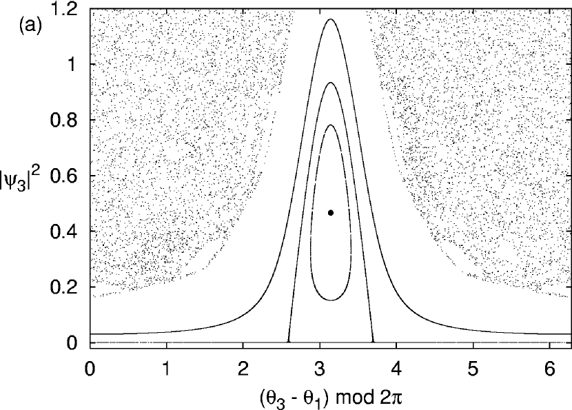
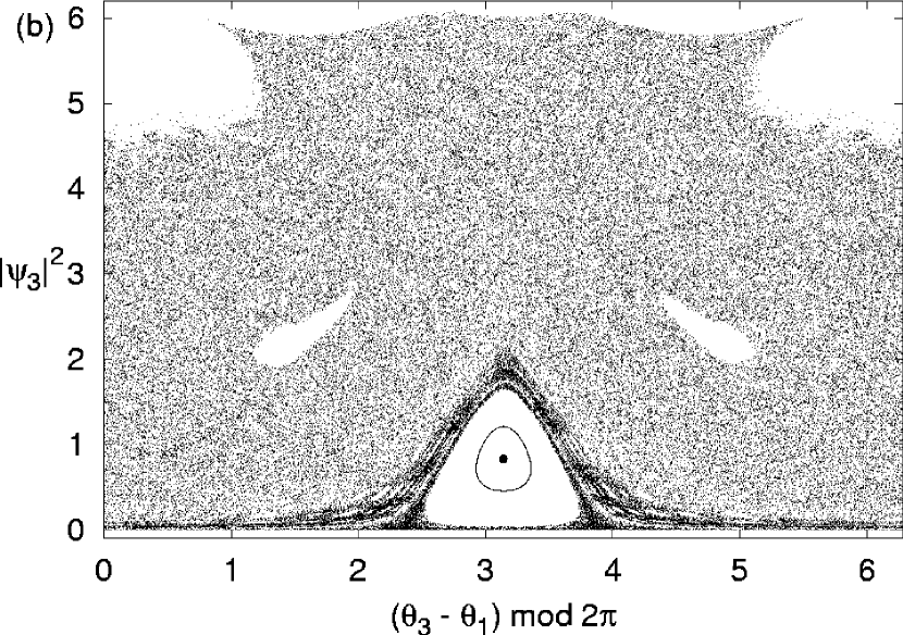
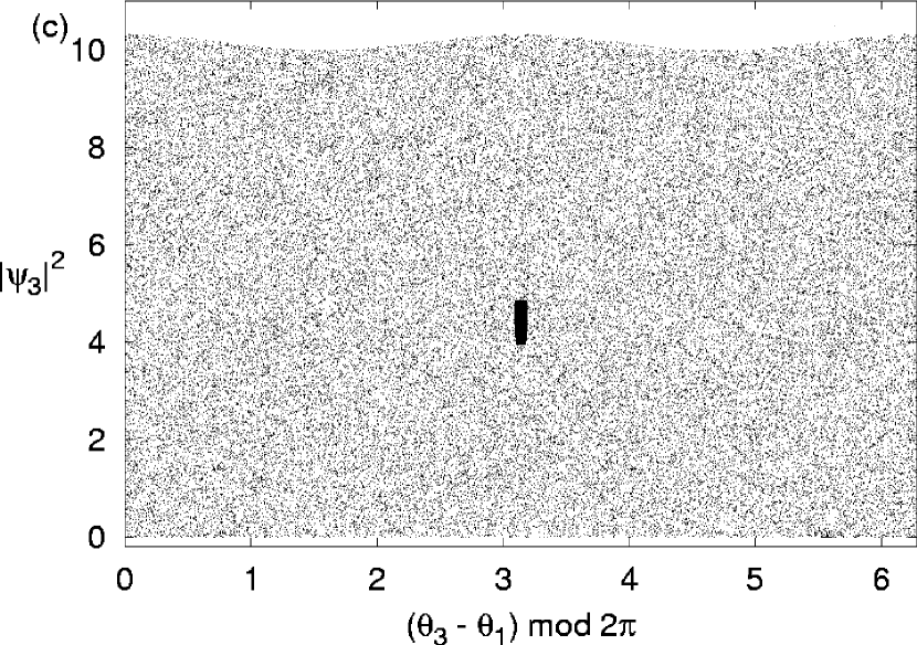
Figure 11: Poincaré sections $\theta_{2}-\theta_{1}=\pi$, $\frac{\rmd}{\rmd t}(\theta_{2}-\theta_{1})<0$ for the dynamics close to unstable stationary solutions (4) with $C=1$ and (a) ${\mathcal{N}}=10$ ($H=5$), (b) ${\mathcal{N}}=10.7$ ($H=3.4775$), and (c), (d) ${\mathcal{N}}=17$ ($H=-21.25$), respectively. The stationary solution is represented by horizontal lines $|\psi_{3}|^{2}=0$. The elliptic fixed point (filled circle) represents continuations of the stable branch of two-frequency solutions in figures 3-4. The window of regular orbits in (d) is marked by a short vertical black line in (c).

Since the stationary solution has zero amplitude at $n=3$ its phase $\theta_{3}$ is undefined, and thus it is represented by a horizontal line $|\psi_{3}|^{2}=0$. The scenario in the self-trapped regime is illustrated by figure 11 (a), corresponding to the dynamics in figure 10 (a). Here the elliptic fixed point at $\theta_{3}-\theta_{1}=\pi$ represents the stable two-frequency solution of section 3.1 with the same value of $H$ as the stationary solution. As in figure 3 (d) this solution belongs to the black branch. This elliptic fixed point appears at $|\psi_{3}|^{2}=0$ at the type I HH bifurcation point ${\mathcal{N}}/C\approx 9.077$, and moves vertically in the direction of increasing $|\psi_{3}|^{2}$ for increasing ${\mathcal{N}}/C$ (cf. figure 3 (b)). It is surrounded by two different kinds of regular periodic or quasiperiodic orbits, where the latter constitute KAM tori corresponding generically to quasiperiodic three-frequency solutions in the original DNLS dynamics. With a pendulum analogy, these orbits can be classified as ’rotating’ and ’vibrating’, respectively, where the former extend for all values of $\theta_{3}-\theta_{1}$ while the latter only exist in a bounded region close to $\theta_{3}-\theta_{1}=\pi$. Then, the unstable stationary solution becomes the separatrix between these different kinds of solutions. Although the separatrix is chaotic (which can be seen from a careful look at figure 11 (a)) the chaos is confined between KAM-tori, and in particular the existence of confining ’rotating’ tori makes it impossible for $|\psi_{3}|^{2}$ to exceed some upper limit value ($|\psi_{3}|^{2}\approx 1$ at $\theta_{3}-\theta_{1}=\pi$ in figure 11 (a)). Thus, self-trapping results.

Below ${\mathcal{N}}/C\approx 9.077$, where the stationary solution is stable and the elliptic fixed point with nonzero $|\psi_{3}|^{2}$ not yet born, all surrounding KAM tori are of the ’rotating’ kind. As ${\mathcal{N}}/C$ is increased and the elliptic fixed point moves upwards towards larger $|\psi_{3}|^{2}$, more and more of the ’rotating’ KAM tori get destroyed, and finally at ${\mathcal{N}}/C\approx 10.6$ the last ’rotating’ KAM torus breaks up, and the self-trapping is destroyed. The Poincaré plot for ${\mathcal{N}}/C=10.7$, i.e. just above the transition point, is shown in figure 11 (b) (the corresponding dynamics is qualitatively similar to figure 10 (b) but with a longer transient $t\sim 17000$). It can be seen, that although the dynamics finally spreads to a large part of the available phase space, the darker parts signifies regions where it will be almost trapped for long times. This should be expected close to the transition point, as destroyed KAM tori should transform into cantori by a transition by breaking of analyticity [63]. Close to the transition the cantori should have almost full measure, and can thus trap the dynamics for very long times. (The white regions in the upper part around $\theta_{3}-\theta_{1}=0$ mod $2\pi$ correspond to dynamics trapped around the equivalent two-frequency solution with main amplitudes at sites $n=2$ and $n=3$.)

At the self-trapping transition ${\mathcal{N}}/C\approx 10.6$, the solution family represented by the elliptic fixed point in figure 11 changes from the black (larger $H$) to the grey (smaller $H$) branch (cf. section 3.1.3 and figure 4 (b)). Increasing further ${\mathcal{N}}/C$, this fixed point continues to move towards larger $|\psi_{3}|^{2}$ (cf. figure 4 (a)), and the surrounding island of KAM tori shrinks so that the unstable stationary solution invades almost all the available phase space (figure 11 (c), (d), corresponding to the dynamics of figure 10 (c)). Here, there are no visible traces of destroyed rotating KAM tori (if cantori exist they should have very small measure), so the dynamics shows no transient trapping. This behaviour persists until the stationary solution regains stability through the type II HH bifurcation at ${\mathcal{N}}/C=18$. Before, at ${\mathcal{N}}/C\approx 17.2$, the grey two-frequency solution becomes unstable through a period-doubling type bifurcation (cf. collision at $\beta=-1$ in figure 4 (c)), so that the elliptic fixed point in figure 11 (d) becomes hyperbolic and splits into two new elliptic points surrounded by tiny KAM tori.

5 Conclusions

In conclusion, we have investigated the Hamiltonian Hopf bifurcations in the three-site DNLS model, resulting in a regime of oscillatory instability for the stationary solution with two sites of anti-phased oscillations and the third site of zero amplitude (’single depleted well’ [53]). Using numerical continuation techniques to calculate the (generally quasiperiodic) two-frequency solutions involved in the two bifurcations, we found them to be of two different types. At the low-amplitude instability threshold the bifurcation is of ’type I’, with stable two-frequency solutions close to the unstable stationary solution near the bifurcation point. These two-frequency solutions are themselves surrounded by KAM tori, representing generally quasiperiodic three-frequency solutions of the full DNLS model. At the high-amplitude instability boundary, the HH bifurcation is of ’type II’, and the stationary solution has no surrounding two-frequency solutions on the unstable side of the bifurcation. This reflects itself as a self-trapping transition in the instability-induced dynamics of the stationary solution, so that in the low-amplitude instability regime the dynamics remains trapped close to the initial state with small amplitude on the third site, while in the high-amplitude instability regime an ’intermittent population inversion’ dynamics is observed with the small-amplitude oscillation moving chaotically between the sites. This self-trapping transition, which we believe has not been described earlier in the literature, was found to correspond to the destruction of phase-space dividing KAM tori.

As discussed in the introduction, our original motivation was to obtain an increased understanding for the dynamics resulting from oscillatory instabilities of certain multibreather configurations in infinite lattices, which have been discovered recently in many contexts. Based on the results obtained here, we will address these issues in a forthcoming publication. However, the three-site DNLS model is of interest in itself, in particular in view of the recent experimental progress in the fields of coupled optical waveguides and Bose-Einstein condensates. It seems likely, that the existence of stable families of two-frequency solutions, corresponding to intensities periodically oscillating around their mean values, as well as the existence of a new type of self-trapping transition in the unstable dynamics of the stationary solution, should be experimentally verifiable within these contexts.

References

References

- [1] Marín J L, Aubry S and Floría L M 1998 Physica D 113 283–92
- [2] Marín J L and Aubry S 1998 Physica D 119 163–74
- [3] Johansson M and Kivshar Yu S 1999 Phys. Rev. Lett.82 85–8
- [4] Morgante A M, Johansson M, Kopidakis G and Aubry S 2000 Phys. Rev. Lett.85 550–3
- [5] Kevrekidis P G, Bishop A R and Rasmussen K Ø 2001 Phys. Rev.E 63 036603-1–6
- [6] Malomed B and Kevrekidis P G 2001 Phys. Rev.E 64 026601-1–6
- [7] Morgante A M, Johansson M, Kopidakis G and Aubry S 2002 Physica D 162 53–94
- [8] Johansson M, Morgante A M, Aubry S and Kopidakis G 2002 Eur. Phys. J. B 29 279–83
- [9] Alvarez A, Archilla J F R, Cuevas J and Romero F R 2002 New J. Phys.4 72.1–19
- [10] MacKay R S and Aubry S 1994 Nonlinearity7 1623–43
- [11] Aubry S 1997 Physica D 103 201–50
- [12] Marín J L and Aubry S 1996 Nonlinearity9 1501–28
- [13] Cretegny T and Aubry S 1997 Phys. Rev.B 55 R11929–32
- [14] Johansson M and Aubry S 1997 Nonlinearity10 1151–78
- [15] Ahn T, MacKay R S and Sepulchre J-A 2001 Nonlinear Dyn. 25 157–82
- [16] Darmanyan S, Kobyakov A and Lederer F 1998 JETP 86 682–6
- [17] Kivshar Yu S, Królikowski W and Chubykalo O A 1994 Phys. Rev.E 50 5020–32
- [18] Johansson M, Aubry S, Gaididei Yu B, Christiansen P L and Rasmussen K Ø 1998 Physica D 119 115–24
- [19] Howard J E and MacKay R S 1987 J. Math. Phys.28 1036–51
- [20] Bridges T J 1997 Proc. R. Soc. Lond. A 453 1365–95
- [21] Kivshar Yu S and Peyrard M 1992 Phys. Rev.A 46 3198–205
- [22] [] Daumont I, Dauxois T and Peyrard M 1997 Nonlinearity10 617–30
- [23] Carr J and Eilbeck J C 1985 Phys. Lett.109A 201–4
- [24] Eilbeck J C, Lomdahl P S and Scott A C 1985 Physica 16D 318–38
- [25] MacKay R S 1986 Nonlinear Phenomena and Chaos ed S Sarkar (Bristol: Adam Hilger) pp 254–70
- [26] [] (reprinted in 1987 Hamiltonian Dynamical Systems ed R S MacKay and J D Meiss (Bristol: Adam Hilger) pp 137–153)
- [27] Bridges T J 1990 Math. Proc. Camb. Phil. Soc. 108 575–601
- [28] Bridges T J 1991 Math. Proc. Camb. Phil. Soc. 109 375–403
- [29] van der Meer J-C 1985 The Hamiltonian Hopf Bifurcation (Berlin: Springer)
- [30] Lahiri A and Roy M S 2001 International Journal of Non-Linear Mechanics 36 787–802
- [31] Arnol’d V I and Sevryuk M B 1986 Nonlinear Phenomena in Plasma Physics and Hydrodynamics ed R Z Sagdeev (Moscow: Mir) pp 31–64
- [32] []Sevryuk M B 1986 Reversible Systems (Berlin: Springer) Chapter 6
- [33] Bambusi D and Vella D 2002 Disc. Cont. Dyn. Syst. -B 2 389–99
- [34] De Filippo S, Fusco Girard M and Salerno M 1989 Nonlinearity2 477–87
- [35] Cruzeiro-Hansson L, Feddersen H, Flesch R, Christiansen P L, Salerno M and Scott A C 1990 Phys. Rev.B 42 522–26
- [36] Hennig D 1992 J. Phys. A: Math. Gen.25 1247–57
- [37] [] Hennig D, Gabriel H, Jørgensen M F, Christiansen P L and Clausen C B 1995 Phys. Rev.E 51 2870–6
- [38] Andersen J D and Kenkre V M 1993 Phys. Rev.B 47 11 134–42
- [39] [] Andersen J D and Kenkre V M 1993 Phys. Status Solidi(b) 177 397–404
- [40] Molina M I and Tsironis G P 1993 Physica D 65 267–73.
- [41] Nemoto K, Holmes C A, Milburn G J and Munro W J 2001 Phys. Rev.A 63 013604-1–6
- [42] Franzosi R and Penna V 2001 Phys. Rev.A 65 013601-1–5
- [43] [] Franzosi R and Penna V 2002 Laser Physics 12 71–6
- [44] Kevrekidis P G, Rasmussen K Ø and Bishop A R 2001 Int. J. Mod. Phys. B 15 2833–900
- [45] Eilbeck J C and Johansson M 2003 Proc. of the 3rd Conf. Localization & Energy Transfer in Nonlinear Systems (June 17–21 2002, San Lorenzo de El Escorial Madrid) ed L Vázquez et al (New Jersey: World Scientific) pp 44–67
- [46] [](Eilbeck J C and Johansson M 2002 Preprint nlin.PS/0211049)
- [47] Christodoulides D N and Joseph R I 1988 Opt. Lett. 13 794–6
- [48] Eisenberg H S, Silberberg Y, Morandotti R, Boyd A R and Aitchison J S 1998 Phys. Rev. Lett.81 3383–6
- [49] []Morandotti R, Peschel U, Aitchison J S, Eisenberg H S and Silberberg Y 1999 Phys. Rev. Lett.83 2726–9
- [50] Smerzi A, Fantoni S, Giovanazzi S and Shenoy S R 1997 Phys. Rev. Lett.79 4950–3
- [51] []Trombettoni A and Smerzi A 2001 Phys. Rev. Lett.86 2353–6
- [52] Abdullaev F Kh, Baizakov B B, Darmanyan S A, Konotop V V and Salerno M 2001 Phys. Rev.A 64 043606-1–10
- [53] Franzosi R and Penna V 2003 Phys. Rev.E 67 046227-1–16
- [54] [](Franzosi R and Penna V 2002 Preprint cond-mat/0203509)
- [55] Eilbeck J C 1987 Physics of Many-Particle Systems 12 ed A Davydov pp 41–51
- [56] [] Eilbeck J C and Scott A C 1989 Structure, Coherence and Chaos in Dynamical Systems ed P L Christiansen and R D Parmentier (Manchester: Manchester University Press) pp 139–59
- [57] Johansson M and Aubry S 2000 Phys. Rev.E 61 5864–79
- [58] Laedke E W, Spatschek K H and Turitsyn S 1994 Phys. Rev. Lett.73 1055–9
- [59] [] Laedke E W, Kluth O and Spatschek K H 1996 Phys. Rev.E 54 4299–311
- [60] Morgante A M, Johansson M, Aubry S and Kopidakis G 2002 J. Phys. A: Math. Gen.35 4999–5021
- [61] Feddersen H, Christiansen P L and Salerno M 1991 Physica Scripta 43 353–5
- [62] Hennig D and Gabriel H 1995 J. Phys. A: Math. Gen.28 3749–56
- [63] Aubry S 1978 Solitons and Condensed Matter Physics ed A R Bishop and T Schneider (Berlin: Springer) pp 264–78