Perturbation of coupling matrices and its effect on the synchronizability in arrays of coupled chaotic systems.

Abstract

In a recent paper, wavelet analysis was used to perturb the coupling matrix in an array of identical chaotic systems in order to improve its synchronization. As the synchronization criterion is determined by the second smallest eigenvalue $\lambda_{2}$ of the coupling matrix, the problem is equivalent to studying how $\lambda_{2}$ of the coupling matrix changes with perturbation. In the aforementioned paper, a small percentage of the wavelet coefficients are modified. However, this result in a perturbed matrix where every element is modified and nonzero. The purpose of this paper is to present some results on the change of $\lambda_{2}$ due to perturbation. In particular, we show that as the number of systems $n\rightarrow\infty$, perturbations which only add local coupling will not change $\lambda_{2}$. On the other hand, we show that there exists perturbations which affect an arbitrarily small percentage of matrix elements, each of which is changed by an arbitrarily small amount and yet can make $\lambda_{2}$ arbitrarily large. These results give conditions on what the perturbation should be in order to improve the synchronizability in an array of coupled chaotic systems. This analysis allows us to prove and explain some of the synchronization phenomena observed in a recently studied network where random coupling are added to a locally connected array. Finally we classify various classes of coupling matrices such as small world networks and scale free networks according to their synchronizability in the limit.

1 Introduction

The object of interest in this paper is a coupled array of $n$ identical systems with linear coupling:

$$\dot{x}=\left(\begin{array}[]{c}f(x_{1},t)\\ \vdots\\ f(x_{n},t)\end{array}\right)-(G\otimes D)x$$ (1)

where $x=(x_{1},\dots,x_{n})$. The coupling matrix $G$ describes the coupling topology of the array, i.e. $G_{ij}\neq 0$ if there is a coupling between system $x_{i}$ and system $x_{j}$. If $G_{ij}<0$ or $G_{ij}>0$, we call such a coupling element cooperative or competitive respectively. In this paper we assume that $G$ is a symmetric zero row sums matrix whose off-diagonal elements are all nonpositive. This implies that all coupling is cooperative and all eigenvalues of $G$ are real. The matrix $D$ describes the coupling between a pair of systems. In [1, 2, 3] it was shown that for a suitable $D$ (such as $D=I$), the synchronization criterion depends solely on the second smallest eigenvalue of $G$, which we denote as $\lambda_{2}(G)$. In particular, the larger $\lambda_{2}(G)$ is, the easier it is to synchronize the array. Furthermore, when the single uncoupled system $\dot{y}=f(y,t)$ is a chaotic system, $\lambda_{2}$ must necessarily be positive in order for the array to synchronize. Therefore we will equate $\lambda_{2}$ with synchronizability in the remainder of this paper. In [1] several coupling topologies were considered. In particular, for nearest neighbor coupling, $\lambda_{2}\rightarrow 0$ as $n\rightarrow\infty$ and thus such an array of chaotic systems will not synchronize for large $n$.

In [4] it was shown using wavelet analysis how a perturbed coupling matrix $\tilde{G}=G+\Delta G$ can be constructed such that $\lambda_{2}(\tilde{G})$ is much larger than $\lambda_{2}(G)$ and thus the synchronizability is greatly improved. The perturbation $\Delta G$ can be thought of as the additional coupling added to the coupling array to affect its synchronization properties. In [4], $\tilde{G}$ is obtained by modifying a small fraction (the $LL_{1}$ subspace) of the wavelet coefficients of $G$. However, all of the matrix elements of $G$ are changed in the process, i.e. $\Delta G$ is not sparse. In particular, there are no zero elements in $\tilde{G}$, the perturbed array is fully connected and every chaotic system is connected to every other chaotic system. To illustrate the increase of $\lambda_{2}$, in [4] the $LL_{1}$ coefficients are multiplied by a factor of $1101$. This results in a full matrix $\tilde{G}$ whose off-diagonal elements are up to 8 times larger than the original matrix $G$. With such drastic changes to $G$, it is not surprising that $\lambda_{2}$ will also change dramatically.

Note that Eq. (1) has a minus sign in front of the term $(G\otimes D)x$ as opposed to a plus sign in [4]. This means that the coupling matrix here is the negative of the coupling matrix in [4]. In other words, whereas [4] talks about the second largest eigenvalue, we consider the second smallest eigenvalue. Writing the state equation as in Eq. (1) has the benefit that $\lambda_{2}$ is positive (rather than negative as in [4]). Furthermore, in this way, $G$ and $\lambda_{2}$ correspond to the graph-theoretical notions of Laplacian matrix and algebraic connectivity respectively [5]. This is notationally less cumbersome later on when we use results from the theory of random graphs.

The purpose of this paper is to attempt to answer the question of what type of matrices $\Delta G$ will make $\lambda_{2}(\tilde{G})$ much larger than $\lambda_{2}(G)$, i.e. greatly improve the synchronizability while keeping $\Delta G$ “small”. This notion of smallness could be the sparseness of $\Delta G$ as this refers to the number of additional coupling added to the original array. It could also be the size of the off-diagonal elements of $\Delta G$ as they relate to the coupling strengths between the chaotic systems in the array. We will show that there exists sparse matrices $\Delta G$ with small elements that will change $\lambda_{2}(G)$ significantly. We also show that uniform coupling will increase the synchronizability the most. On the other hand, we show that local coupling, i.e. $\tilde{G}$ corresponding to a graph with only local connections, will not synchronize when the number of systems is large.

We also show how this analysis allows us to prove and explain the change in synchronizability observed in a coupled array where random coupling elements are added to a nearest neighbor coupled array.

Finally we will classify several classes of coupling matrices considered in the literature according to a synchronizability measure, and show that the more random and less ordered the coupling graph is, the higher the synchronizability.

2 Super-additivity of $\lambda_{2}$

Definition 1

$W$ is the class of symmetric matrices that have zero row sums and nonpositive off-diagonal elements.

It can be shown that matrices in $W$ are positive semi-definite and that $0$ is a simple eigenvalue if and only if the matrix is irreducible [1]. We assume that the coupling matrices $G$ and $\tilde{G}$ are in $W$.

Lemma 1

If $A$ and $B$ are in $W$, then $\lambda_{2}(A+B)\geq\lambda_{2}(A)+\lambda_{2}(B)$.

Proof: see [1]. $\Box$

This lemma shows that $\lambda_{2}(\tilde{G})\geq\lambda_{2}(G)+\lambda_{2}(\Delta G)$ when $\Delta G$ is also a matrix in $W$. Therefore if we can find $\Delta G$ such that $\lambda_{2}(\Delta G)$ is large, then we can increase $\lambda_{2}(\tilde{G})$ and thus the synchronizability.

A corollary to Lemma 1 is that if $A$, $B$ are matrices in $W$ and every off-diagonal element of $A$ is smaller in absolute value than $B$, then $\lambda_{2}(A)\leq\lambda_{2}(B)$. This means that adding additional cooperative coupling elements ($G_{ij}<0$) can only increase $\lambda_{2}$ and improve the synchronizability.

Let us consider three reasonable constraints on the possible coupling matrix $G$ that we can choose:

1. $G\in W$.

2. the number of nonzero coupling elements is a percentage of the total number of coupling elements, i.e. only a percentage of the off-diagonal elements of $G$ are nonzero.

3. the absolute value of each off-diagonal element is less than some fixed number $B>0$.

Under these constraints, the above discussion shows that the matrix $G$ with the largest $\lambda_{2}$ must necessarily be matrices in $W$ where the off-diagonal elements are either $0$ or $-B$. We call such a coupling configuration a uniform coupling as the coupling between any pair of systems is either zero or the same. Thus given a bound on the size of each coupling element, the uniform coupling is the best coupling configuration in terms of synchronizability.

This motivates us to study the class of matrices in $W$ where the off-diagonal elements is either 0 or -1. Such a matrix is the Laplacian matrix of the underlying graph: vertex $i$ is connected to vertex $j$ if and only if $G_{ij}\neq 0$ and $\lambda_{2}$ corresponds to the algebraic connectivity of the graph [6]. This allows us to use results in graph theory to study $\lambda_{2}(\tilde{G})$. In particular, in the rest of the paper, we will mainly consider coupling matrices which is a positive multiple of the Laplacian matrix of the underlying graph and the goal is to find appropriate coupling graphs whose algebraic connectivity are large.

3 Local coupling

Consider the following model of local coupling [7]: let the vertices of the coupling graph be the points in the hypercube $[0,r]^{d}$ with integer coordinates, i.e. the vertices are the lattice points inside the hypercube $[0,r]^{d}$ generated by the standard basis vectors. Let the systems in the array be located on these vertices. We say this array is locally connected if there exists a fixed $\delta$ such that all the systems which are connected to each system $x$ lies in the $\delta$-neighborhood of $x$. This notion of local coupling includes examples such as nearest neighbor coupling and grid graphs, but also more general local coupling configurations where the vertex degree is bounded but not necessarily constant.

In [7] it was shown that:

Lemma 2

For fixed $d$ and $\delta$, a locally connected array will have $\lambda_{2}\rightarrow 0$ as $n\rightarrow\infty$ (i.e. $r\rightarrow\infty$). This is true even if the hypercube is considered as a hypertorus.

This means that locally connected arrays will have low synchronizability for large $n$. In particular, locally connected arrays of chaotic systems will not synchronize for large $n$. This means that $\Delta G$ should have nonlocal coupling in order to improve the synchronizability of the array. Next we show that random coupling is some sense the best candidate for such nonlocal coupling.

4 Random coupling

How much coupling do we need to add in order to make $\lambda_{2}$ large while keeping the size of the off-diagonal element small? In [6] it was shown that:

Lemma 3

For a non-complete graph $\lambda_{2}$ is less than or equal to the minimum vertex degree.

In particular, for a $k$-regular (non-complete) graph, $\lambda_{2}\leq k$. Therefore, if we want $\lambda_{2}$ to be large we need each vertex to connect to a large number of other vertices, i.e. $\Delta G$ cannot be too sparse. Regular random graphs appear to be asymptotically optimal in this respect by Lemma 3 and the following lemma.

Lemma 4

There exists a constant $0<c<1$ such that almost every $k$-regular random graph satisfies $\lambda_{2}>ck$ as $n\rightarrow\infty$ for large enough $k$. For even $k$, $c$ can be chosen close to $1$.

Proof: See [7]. $\Box$

For small $k$, it can be shown that for $k\geq 3$, there is a constant $c_{k}>0$ such that almost every $k$-regular random graph satisfies $\lambda_{2}\geq c_{k}$ as $n\rightarrow\infty$. In particular, since $\lambda_{2}\geq k-\sqrt{k^{2}-i^{2}}$ [8, 5] where $i$ is the isoperimetric number of the graph, and using the results in [9], a graph of $c_{k}$ for $k$ between $3$ and $15$ is shown in Figure 1.

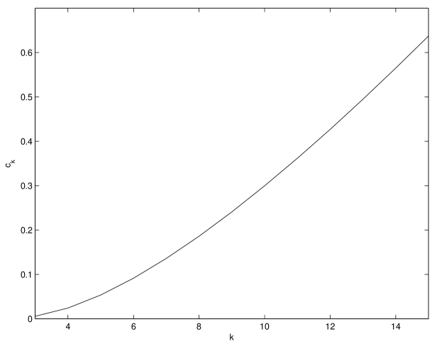
Figure 1: Plot of lower bound $c_{k}$ of the second smallest eigenvalue of $k$-regular random graphs for $3\leq k\leq 15$.

This allows us to prove the following theorem which says that there is an $n$ by $n$ coupling matrix $\Delta G$ with an arbitrarily small percentage of nonzero off-diagonal elements, each of which is arbitrarily small, and which has arbitrarily large $\lambda_{2}$ when $n$ is large enough.

Theorem 1

Given $0<p\leq 1$, $r>0$, and $s$, for all large enough $n$, there exists a matrix $\Delta G$ in $W$ such that

• $\lambda_{2}>s$,

• the fraction of nonzero elements of $\Delta G$ is $p$,

• each off-diagonal element of $\Delta G$ is less than $r$.

Proof: Choose $k$ an integer larger than $\frac{s}{cr}$. By Lemma 4 for large enough $n$ and $k$, almost every random $k$-regular graph will have $\lambda_{2}>\frac{s}{r}$. Choose large $n$ such that $n>\frac{k}{p}$. Let $A$ be the Laplacian matrix of such a graph. Then $\Delta G=rA$ will suffice. $\Box$

So far, the random graph corresponding to $\Delta G$ is required to be a regular graph. Next we show that this requirement can be relaxed. In [10] a network model is presented where a nearest neighbor configuration is modified by adding a fraction $0\leq p\leq 1$ of random edges out of all possible edges. In [10] it was shown via numerical experiments that $\lambda_{2}(\tilde{G})$ increases in a near linear fashion with respect to $p$ and to $n$. We prove that this is true in general. Let $G$ be a locally connected graph and $\Delta G$ is constructed as in [10] by picking randomly a fraction $p$ of all possible edges.

First note that by Lemmas 1 and 3, $\lambda_{2}(\tilde{G})\leq pn+q$ where $q$ is the average number of connections of $G$. In [12] it was shown that $\lambda_{2}(\Delta G)$ is equal to $pn+o(n^{\frac{1}{2}+\epsilon})$ in probability for any $\epsilon>0$. Combining this with Lemmas 1 and 2, it’s clear that $\lambda_{2}(\tilde{G})$ increases as $o(pn)$ in probability as $n\rightarrow\infty$, i.e. linear in $p$ and in $n$.

Thus in general, given a locally connected array, the addition of a fraction of random edges out of all possible edges will increase the synchronizability by an arbitrarily large amount as the number of vertices increases. Note that the synchronizability of the random edges dominates that of the locally connected graph.

4.1 Example

To compare the results in this section with the results in [4], consider the example in [4] that was discussed in Section 1 where an array of 64 oscillators with nearest neighbour coupling is perturbed by multiplying the $LL_{1}$ wavelet coefficients of the coupling matrix $G$ by a factor of $1101$. This increases $\lambda_{2}$ from $0.0096$ to $0.1522$. However, all entries of the 64 by 64 matrix $G$ are changed, with the off-diagonal entries of the perturbation matrix $\Delta G$ ranging from $-7.6$ to $9.7$. On the other hand, suppose we want to change only $5$ percent of the off-diagonal entries of $G$. By choosing a random graph with $100$ edges and corresponding Laplacian matrix $L$, we construct a perturbation matrix $\Delta G=0.0665L$ which also increases $\lambda_{2}$ from $0.0096$ to $0.1522$. However, in this case, only $5$ percent of the off-diagonal entries of $G$ are perturbed, and the off-diagonal entries of the perturbation matrix $\Delta G$ is either $-0.0665$ or $0$. Thus the improvement in synchronization is the same as in [4], but the perturbation matrix is much smaller, both in the sense of the number of nonzero elements and in the sense of the magnitude of the nonzero elements.

5 Comparison of various classes of coupling graphs

In this section we compare several classes of coupling graphs that have been proposed in the literature for modeling complex networks, both man-made (the internet or social networks) and occuring in nature (neural networks). We can categorize their synchronizability by studying the synchronizability measure $s(m)=\lim_{n\rightarrow\infty}\frac{\lambda_{2}}{m}$ when it exists, where $m$ is the average number of connections defined as 2 times the number of edges divided by the number of vertices, i.e. $m$ is the number of nonzero off-diagonal elements of the Laplacian matrix divided by $n$. For $r$-regular graphs, $m=r$. By Lemma 3, $0\leq s(m)\leq 1$. We will only consider the cases $m\geq 3$.

5.1 Small world networks

In [11] a small-world network model is introduced where starting from a locally connected graph with $m$ edges, $pm$ edges ($0<p\leq 1$) are added randomly. Without the random edges $\lambda_{2}\rightarrow 0$ as $n\rightarrow\infty$ by Lemma 2. In the cases considered in [11], $m$ grows linearly with $n$, i.e. $m=kn$. If we modified this model such that the added random edges form a regular random graph, then the discussion in Section 4 shows that $\lambda_{2}$ is bounded away from zero as $n\rightarrow\infty$ when $kp\geq\frac{3}{2}$. In particular, Figure 1 shows that $s(m)\geq 0.0018$. Thus by adding the random edges, there is a coupling strength factor $\epsilon>0$ such that when $D$ is replaced by $\epsilon D$, the coupled array will synchronize independent of $n$.

5.2 Scale-free random networks

In [13] a scale-free random network model of the internet is presented where the graph is built up as follows: Starting from a initial set of $k_{0}$ (usually set at $k_{0}=k$) vertices, at each iteration a new vertex is added with $k$ new edges connecting this vertex to $k$ existing vertices. Thus the average connections is $m=2k$ as $n\rightarrow\infty$. The probability that the new vertex is connected to vertex $i$ is proportional to the vertex degree of vertex $i$. This results in a graph whose vertex degree distribution follows a power law. Since there is always at least one vertex with degree $k$, $\lambda_{2}\leq k$ and $s(m)\leq\frac{1}{2}$ by Lemma 3. Computer simulations show that for a fixed $m$, $\lambda_{2}$ of such graphs appear to increase monotonically as a function of $n$. If this is the case, then since $\lambda_{2}$ is bounded by $\frac{m}{2}$, this means that $\lambda_{2}$ converges to a constant value $\lambda_{2}^{\infty}(m)$ as $n\rightarrow\infty$. We computed via simulations the value of $s(m)=\frac{\lambda_{2}^{\infty}(m)}{m}$ for various $m$ as shown in Figure 2. We see that $s(m)$ is increasing and converging to close to the upper bound $\frac{1}{2}$. As the scale-free network is not as random as a random network, its synchronizability measure is also less.

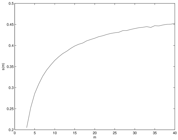
Figure 2: Plot of the synchronizability measure $s(m)$ for scale free random networks. We see that $s(m)$ is increasing and approaches close to the upper bound $\frac{1}{2}$.

For locally connected graphs, $s(m)=0$ for all $m$ by Lemma 2. For both small-world networks and the model in [10] $s(m)\approx 1$ for large $m$. The main difference is that in small-world networks, $m$ (and thus also $\lambda_{2}$) is small and bounded, whereas in [10], $m=pn$ and therefore $\lambda_{2}$ is unbounded. These results are summarized in Table 1.

Graph class	Synchronizability measure $s(m)$
Locally connected graphs [7]	$0$
Scale-free networks [13]	$\approx 0.5$ as $m\rightarrow\infty$
Small world networks [11]	$\geq 0.0018$, $\approx 1$ as $m\rightarrow\infty$
Model in [10]	$s(m)\approx 1$, $\lambda_{2}\rightarrow\infty$ as $n\rightarrow\infty$

Table 1: Several classes of coupling graphs and their synchronizability measure $s(m)$.

Thus we can order these classes of matrices as follows in terms of increasing synchronizability: locally connected graphs, scale-free networks, small-world networks, and the model in [10]. We see that the more disorder and randomness the graph exhibits, the higher the synchronizability.

6 Conclusions

We study the conditions under which perturbation of the coupling in a coupled array results in improved synchronizability by reducing it to the analysis of the second smallest eigenvalue of the coupling matrix. We show that local coupling and random coupling form two extremes in their effect on synchronizability. In particular, local coupling will not improve synchronizability in the limit and random coupling can change the synchronizability using arbitrarily small percentage of coupling elements whose strengths are arbitrarily small. As graphs become less ordered and more random, we see that the synchronizability increases. Furthermore, for graphs which is constructed by adding a random component to a structured component, the super-additivity of $\lambda_{2}$ allows us to give a lower bound for the synchronizability of graphs by adding the synchronizability of each of the components. In particular, when the structured component is a locally connected graph, the synchronizability of the random component dominates the synchronizability of the locally connected component.

References

- [1] C. W. Wu and L. O. Chua, “Synchronization in an array of linearly coupled dynamical systems,” IEEE Transactions on Circuits and Systems–I: Fundamental Theory and Applications, vol. 42, no. 8, pp. 430–447, 1995.
- [2] L. M. Pecora and T. L. Carroll, “Master stability functions for synchronized coupled systems,” Physical Review Letters, vol. 80, no. 10, pp. 2109–2112, 1998.
- [3] C. W. Wu, Synchronization in coupled chaotic circuits and systems. World Scientific, 2002.
- [4] G. W. Wei, M. Zhan, and C.-H. Lai, “Tailoring wavelets for chaos control,” Physical Review Letters, vol. 89, no. 28, p. 284103, 2002.
- [5] C. W. Wu and L. O. Chua, “Application of graph theory to the synchronization in an array of coupled nonlinear oscillators,” IEEE Transactions on Circuits and Systems–I: Fundamental Theory and Applications, vol. 42, pp. 494–497, Aug. 1995.
- [6] M. Fiedler, “Algebraic connectivity of graphs,” Czechoslovak Mathematical Journal, vol. 23, no. 98, pp. 298–305, 1973.
- [7] C. W. Wu, “Synchronization in arrays of coupled nonlinear systems: Passivity, circle criterion and observer design,” IEEE Transactions on Circuits and Systems–I: Fundamental Theory and Applications, vol. 48, no. 10, pp. 1257–1261, 2001.
- [8] B. Mohar, “Isoperimetric numbers of graphs,” Journal of Combinatorial Theory, Series B, vol. 47, pp. 274–291, 1989.
- [9] B. Bollobás, “The isoperimetric number of random regular graphs,” European Journal of Combinatorics, vol. 9, pp. 241–244, 1988.
- [10] X. F. Wang and G. Chen, “Synchronization in small-world dynamical networks,” International Journal of Bifurcation and Chaos, vol. 12, no. 1, pp. 187–192, 2002.
- [11] M. E. J. Newman and D. J. Watts, “Scaling and percolation in the small-world network model,” Physical Review E, vol. 60, no. 6, pp. 7332–7342, 1999.
- [12] F. Juhász, “The asymptotic behaviour of Fiedler’s algebraic connectivity for random graphs,” Discrete Mathematics, vol. 96, pp. 59–63, 1991.
- [13] A.-L. Barabási, R. Albert, and H. Jeong, “Scale-free characteristics of random networks: the topology of the world wide web,” Physica A, vol. 281, pp. 69–77, 2000.