Distribution of injected power fluctuations in electroconvection

Abstract

We report on the distribution spectra of the fluctations in the amount of power injected into a liquid crystal undergoing electroconvective flow. The probability distribution functions (PDFs) of the fluctuations as well as the magnitude of the fluctuations have been determined in a wide range of imposed stress both for ‘unconfined’ and ‘confined’ flow geometries. These spectra are compared to those found in other systems held far from equilibrium, and find that in certain conditions we obtain the ”universal” PDF form reported in [Phys. Rev. Lett. 84, 3744 (2000)]. Moreover, the PDF approaches this universal form via an interesting mechanism whereby the distribution’s negative tail evolves towards form in a different manner than the positive tail.

Fluctuations in systems driven out of equilibrium have recently attracted considerable attention, particularly with regard to the probability density function (PDF) of fluctuations in global quantities. Fluctuations in global quantities are necessarily the result of many individual fluctuating modes, thus the first issue is whether the central limit theorem, which predicts a Gaussian PDF, holds. Recent results in a number of disparate systems reveal non-Gaussian PDF’s exhibiting rich and intriguing behavior. Furthermore, the understanding of such PDF’s is of practical importance, not least because one would like to predict the probability of exceedingly rare fluctuations having colossal amplitude (e.g. floods, violent storms, earthquakes, stockmarket swings). While non-Gaussian PDF’s of fluctuations are intriguing in their own right, recent results suggest there may exist a universal, non-Gaussian distribution of global fluctuations. Strikingly, such a distribution has been found, using no adjusted parameters or fits, for an astonishing variety of seemingly unrelated systems: turbulent flow in confined geometry,[1, 2, 3, 4, 5, 6, 7, 8], the Danube water level,[9] and simulations of the 3D X-Y model at criticality [5, 10, 11]. In all these systems, the PDF is substantially skewed, with one tail well described by an exponential decay. This distribution is well described by generalized Fisher-Tippet-Gumbel (gFTG) distribution [10]. The exponential tail is adduced[5, 6, 12] to be due to fluctuations having length scale comparable to the system size. This explanation is supported by measurements on turbulent swirling flow in unconfined geometry [2], in which no exponential tail has been found and the fluctuations became Gaussian. Note that all the above listed results have been obtained for isotropic fluids.

For flow of anisotropic fluids, velocity fluctuations of tracer particles have been investigated[13] in the so-called soft mode turbulence [14], and with the increase of the stress a change in PDF has been observed from Lévy to Gaussian via some intermediate distributions such as the exponential one. However, it should be borne in mind that these represent local rather than global measurements. Electrohydrodynamic convection (EHC) in liquid crystals (LCs) is a unique system in which abrupt turbulence to turbulence transitions [such as defect turbulence to dynamic scattering mode 1 (DSM1) or DSM1 to DSM2] occur at well defined thresholds. The study of the average injected power and fluctuations in quantity in EHC has been established in Refs. [15, 16, 17]. This method opens new routes in investigations of EHC. In this Letter we analyze the PDF of fluctuations in an anisotropic fluid system driven far out of equilibrium. EHC affords the opportunity of varying the externally imposed stress over a sufficiently wide range that it is possible to observe the evolution of the PDF shape. Furthermore, our system allows detailed studies of the effects of confinement on the PDF evolution. The latter is important because the experimental results of Ref. [2] show substantial, qualitative differences between PDF forms for fluctuations of global injected power in ‘unconfined’ and in ‘confined’ geometries.

In turbulent swirling flow experiments in which the fluctuations in injected power are measured, the stress applied to the fluid is characterized by the Reynolds number ($Re$). The comparison of PDF between confined and unconfined flow was made over a range of $Re$ less than 10 [2]. Direct comparison with EHC is problematic because the stress applied to the LC inducing flow is characterized by not by a Reynolds number but rather by the dimensionless potential difference, $\varepsilon\equiv U^{2}/U_{c}^{2}-1$, where $U$ is the applied potential difference and $U_{c}$ is the critical potential difference necessary to induce flow. Two important advantages of EHC are, the ability to widely vary both the relevant length scales and $\varepsilon$.

Our experimental setup is described in Ref. [16]. A sinusoidal voltage signal is amplified and applied across the LC layer sandwiched between two glass plates. The current traversing through the LC sample returns to ground via the field-effect transistor input of a current-to-voltage preamplifier. The output of this preamplifier is measured by a lock-in amplifier whose reference signal is is supplied by the original function generator. The in-phase output of the lock-in is amplified and digitized. For each experimental point an optical image taken through a polarizing microscope with shadowgraph technique has been also recorded. The liquid crystalline mixture Mischung V (MV) with $2.73wt\%$ dopant has been used which is an excellent model material because of its chemical stability and known material parameters [18]. All the measurements presented below have been carried out at temperature $T=(50.00\pm 0.01)^{\circ}C$, where a satisfactory spatial homogeneity of the sample is ensured [19]. The LC is encased in sandwich-type cells with planar orientation for both ‘unconfined’, and ‘confined’ flow geometry. For ‘unconfined’ flow geometry, we chose a cell with square, etched electrodes having active area $A=(6.15\pm 0.1)mm^{2}$ and thickness of $d=(33.4\pm 0.2)\mu m$. In this geometry, the electric field is present and the convection takes place within the active area. This area is laterally bounded by the remainder of the LC, thus the flow and director fields are not controlled at these boundaries. For the ‘confined’ flow geometry, a mylar gasket with a circular hole [$A=(24.6\pm 0.6)mm^{2}$] was used to confine the LC between the conductive plates and within the active area. The separation between the plates was $d=(80\pm 20)\mu m$. The above described dimensions provide aspect ratios $s=\sqrt{A}/d\approx 74$ for the ‘unconfined’ flow geometry and $s\approx 62$ for the ‘confined’ cell. These values of $s$ are similar enough to make quantitative comparison for injected power fluctuations between the ‘unconfined’ and ‘confined’ geometry, knowing that the normalized variance of power fluctuations depends strongly on $s$ [20]. Before performing fluctuation measurements, the experimental setup was tested by replacing the LC sample with 100M$\Omega$ ohmic resistor (resistivity of the same order of magnitude as our samples). Fluctuations in the current injected into the test resistor obey Gaussian statistics with $\sigma_{P}/\langle P\rangle~{}<~{}10^{-5}$.

Figure 1 shows temporal dependence of the normalized power fluctuations around the mean value $\langle P\rangle$ for both unconfined and confined LC electroconvective flow at moderate stress: $\varepsilon=42$. We want to emphasize two features of these fluctuations. First, the normalized variance of fluctuations $\sigma_{P}/\langle P\rangle=\sqrt{(P-\langle P\rangle)^{2}}/\langle P\rangle$ is of the same order of magnitude for unconfined and confined flow. We do not witness the significant increase in $\sigma_{P}/\langle P\rangle$ when the flow is confined as described in Ref. [2]. Second, there is a qualitative difference between the power fluctuations in the two flow geometries. For unconfined flow (at this value of $\varepsilon$) injected power fluctuations are uniform, resulting in almost Gaussian PDF (see below). In contrast, during confined flow, we observe relatively rare but intermittent fluctuations having large, negative amplitude (at least 6.5 standard deviations); these negatively skew the PDF which appears to be well described by the gFTG.

Before discussing the forms of PDF, it is useful to summarize the results of the optical observations (performed concomitantly with the injected power fluctuation measurements). In general, the EHC patterns have similar appearance in unconfined and in confined flow geometry however, they appear at somewhat different values of $\varepsilon$ for the two geometries and they differ in details within the defect turbulence regime (e.g., the grid pattern is observed in unconfined flow but not in confined flow). In both geometries, as $\varepsilon$ is increased above zero the stationary, oblique roll pattern appears. Defect turbulence (described more in detail below) starts at $\varepsilon\approx 0.2$ for both flow geometries. Defect turbulence is characterized by low-frequency, persistent oscillations in the autocorrelation function $g_{a}(t)$ of the power fluctuations [20]. The transition threshold from defect turbulence to DSM1 is defined as the voltage $\varepsilon$ at which the persistent oscillations in $g_{a}(t)$ diminish [20]. This transition occurs at $\varepsilon\approx 7.7$ and at $\varepsilon\approx 12.5$ for the unconfined and confined flow, respectively. The DSM1 $\rightarrow$ DSM2 turbulence transition (involving an abrupt increase in density of disclination loops) has been detected at $\varepsilon\equiv\varepsilon_{t}\approx 62$ and at $\varepsilon_{t}\approx 19.9$ for the unconfined and confined flow, respectively. With further increase of $\varepsilon$ no more transitions are reported in the literature. This is unsurprising because above $\varepsilon\approx 800$ the flow becomes so turbid that is is impossible to visually detect any further change in the pattern.

Figures 2 and 3 show PDFs of injected power fluctuations $\pi(P)$ scaled with their variance $\sigma_{P}$ as a function of power around its mean value $\langle P\rangle$ normalized with $\sigma_{P}$ at different imposed stresses covering a range of about $10^{3}$ for both unconfined (open symbols) and confined flow (closed symbols). The full lines are Gaussian distributions as denoted in Fig. 2(a) with the same $\sigma_{P}$ as experimental results (not fits). The dashed lines are the gFTG distribution:

$$\pi(P)\sigma_{P}=K\exp(b(x-c)-e^{b(x-c)})^{a}$$ (1)

where $x=(P-\langle P\rangle)/\sigma_{P}$, $K=2.14$, $a=\pi/2$, $b=0.938$ and $c=0.374$. This is not a fit: all parameter values are taken from [10]. This is the distribution referred to as “universal” in Ref. [10].

Slightly above EHC threshold, at $\varepsilon\approx 0.2$ the process of generation/annihilation of defects (dislocations) starts which destroys the stationary EHC roll pattern by breaking the rolls into moving segments and leading to a state called defect turbulence [23]. Defect turbulence causes dramatic increase in the amplitude of power fluctuations and the fluctuations become quasi-periodic with a dominant frequency corresponding to the defect lifetime [20]. These fluctuations are well described by Gaussian distribution for both the unconfined and confined flow geometry; see Fig. 2(a).

With further increase of $\varepsilon$, the PDF for unconfined flow remains Gaussian even above the defect turbulence $\rightarrow$ DSM1 transition – see Figs. 2(b) and 2(c). Figure 2(d) shows PDFs obtained at $\varepsilon=42$ (corresponding to Fig. 1). In the unconfined flow, we are deeply in DSM1, and at this $\varepsilon$ the first systematic departure from the Gaussian distribution is observed with tails on decaying slower than Gaussian on both sides of the PDF. With further increase of $\varepsilon$, but still staying in DSM1 turbulence the deviation from the normal distribution becomes even more pronounced [Fig. 3(a)]. At and above $\varepsilon_{t}\approx 62$, the PDF for unconfined flow abruptly reverts to Gaussian [Fig. 3(b)] and remains so for $\varepsilon$ up to about 860. Above this value, the PDF deviates again from Gaussian and its form is much closer to gFTG.[10] (c.f. Fig. 3(c)); the PDF keeps this shape for extremely high $\varepsilon>1000$, [Fig. 3(d), open symbols, $\varepsilon=1717$].

In stark contrast, in the confined flow geometry, a systematic deviation from the Gaussian distribution is detected even in the defect turbulence regime, above $\varepsilon\approx 4$ [closed symbols in Fig. 2(b)]. This deviation reminds us of the results obtained for swirling flow in confined geometry[2]. Clearly, the negative tail of PDF for confined flow in Fig. 2(b) is exponential and is in agreement with gFTG distribution. The positive tail however, remains Gaussian. Thus, at this range of stress we observe a “hybrid” distribution having gFTG tail for negative fluctuations but a Gaussian tail for positive fluctuations. The deviation from Gaussian distribution (and convergence to gFTG) is even more expressed above the defect turbulence $\rightarrow$ DSM1 transition [closed symbols in Fig. 2(c)], where the positive tail also starts to approach the gFTG distribution. In contrast to the unconfined flow geometry, in confined flow DSM1 $\rightarrow$ DSM2 transition has no noticeable influence on the form of PDF [cf. Figs. 2(c) and 2(d)] which stays close to gFTG distribution up to $\varepsilon\approx 1000$ (over a range of $O(10^{3})$ of imposed stress) [Figs. 2(d) and 3(a)–(c)]. At extremely high stresses ($\varepsilon>1000$) however, the form of PDF changes and the typical shape is shown in Fig. 3(d) (closed symbols, $\varepsilon=1424$) with heavy tails on both negative and positive sides.

The Gaussian PDFs in Fig 2(a) for both confined and unconfined flow suggest that fluctuations in global injected power arise from many spatially uncorrelated contributions (defects). However, despite the spatial uncorrelation in defect turbulence, there is still a surprising degree of temporal order embedded[19, 20]. Figs. 2(b) and 2(c) are in the agreement with the results of Ref. [2] for swirling flow: for unconfined flows the PDF is Gaussian, for confined flow however, it is much closer to gFTG distribution. The PDF for confined flow stays remarkably close to the gFTG distribution for $\varepsilon$ varying over $\approx 10^{3}$ [Figs. 2(b)-(d) and 3(a)-(c), closed symbols]. Above $\varepsilon\approx 1000$ however, the PDF changes; rare events of large amplitude fluctuations no longer follow the gFTG distribution; instead they form the above mentioned PDF with heavy tails [Fig. 3(d)]. For unconfined flow, the PDF remains Gaussian over a range of $\varepsilon>10^{2}$ except in a narrow range of $\varepsilon$ just below the threshold of DSM1 $\rightarrow$ DSM2 turbulence transition [Figs. 2(d) and 3(a)]. At high $\varepsilon$ however, PDF of unconfined flow also follows gFTG distribution [Figs. 3(c)-(d)]. Furthermore, the skewness of the measured distributions is $-(0.91\pm 0.2)$ and $-(1.0\pm 0.1)$ for unconfined ($\varepsilon>860$) and confined ($5<\varepsilon<1000$), which compares variably with the expected value for the gFTG of -0.893.

The results discussed above have several implications. First, the gFTG distribution of global fluctuations is observable even in unconfined flow, but at substantially larger imposed stress. This suggests even more strongly that this distribution may be a universal trend for strongly fluctuating non-equilibrium systems, whether the flow is confined or not. Second, when the imposed stress is sufficiently increased, we observe departures from the gFTG distribution. Thus, this distribution, while exhibiting indications of being universal (in that the same form is observed for disparate systems) cannot be thought of as a limiting, ultimate shape. Interestingly, we have shown that the form of PDF is not simply dependent on the boundary conditions and the applied stress, but in our system also depends on turbulence to turbulence transition(s) [c.f. Figs. 3(a) and (b)]. Of course, such transitions are not common. Last, the confined flow experiments above reveal a fascinating mechanism whereby the PDF transforms as the stress is increased. Starting with Gaussian at low stress, the PDF morphs into a hybrid distribution in which the negative fluctuations follow the exponential decay of the gFTG, while the positive fluctuations remain Gaussian. As the stress increases, the positive fluctuations then decay more quickly than Gaussian, and the gFTG is obtained. We are unaware of any theoretical explanations of such transitions between PDF’s.

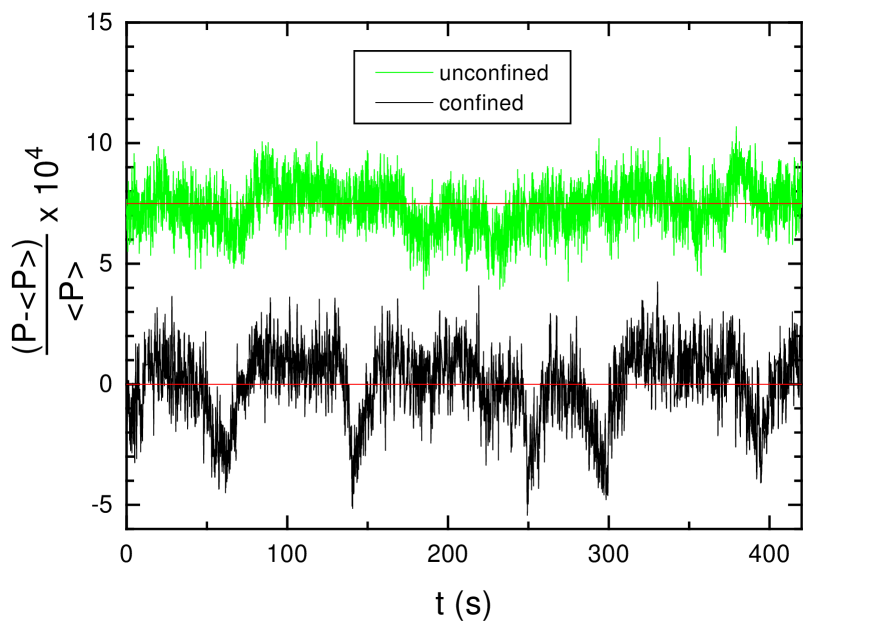
FIG. 1.: Temporal dependence of normalized injected power fluctuations around the mean value $\langle P\rangle$ for unconfined flow (offset by $7.5\times 10^{-4}$) and for confined flow geometry at $\varepsilon=42$.

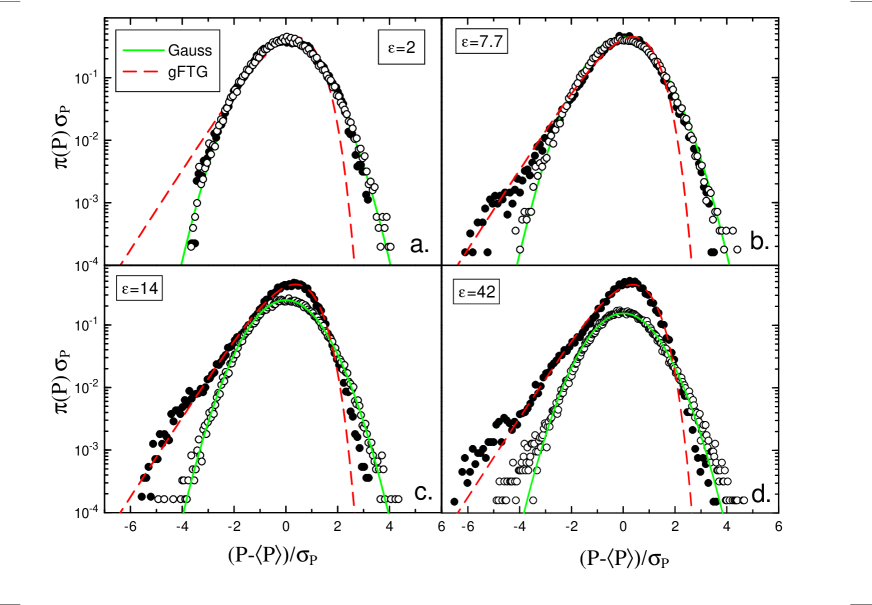
FIG. 2.: Probability density function for both unconfined (open symbols) and confined flow geometry (closed symbols). Lines show Gaussian and gFTG distributions as denoted in legend. (a) $\varepsilon=2$ – defect turbulence for both geometry; (b) $\varepsilon=7.7$ – DSM1 for unconfined flow and defect turbulence for confined flow; (c) $\varepsilon=14$ – DSM1 for both unconfined and confined flow; (d) $\varepsilon=42$ – DSM1 for unconfined flow and DSM2 for confined flow.

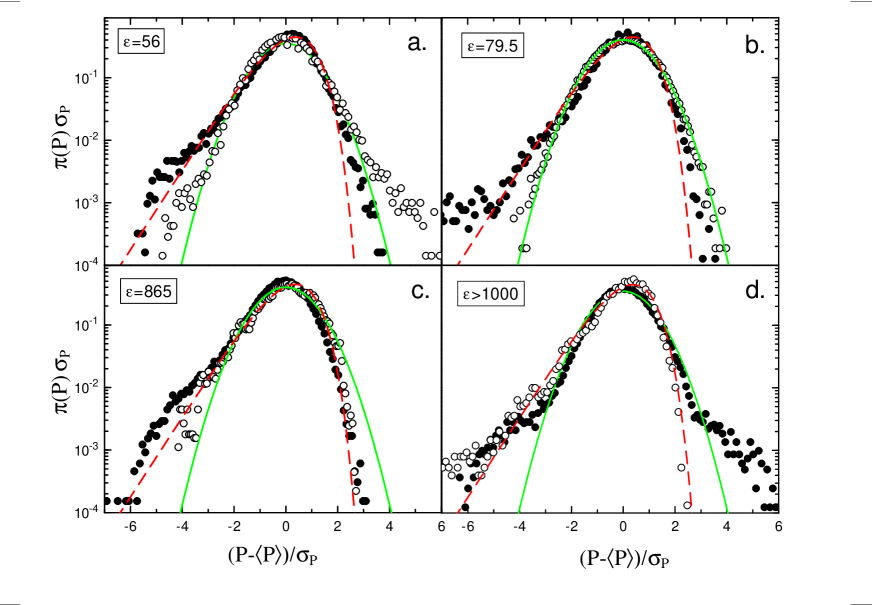
FIG. 3.: Same as Fig. 2, at higher values of $\varepsilon$. (a) $\varepsilon=56$ – DSM1 for unconfined flow and DSM2 for confined flow; (b) $\varepsilon=79.5$ – DSM2 for both unconfined and confined flow; (c) $\varepsilon=865$ – DSM2 for both unconfined and confined flow; (d) $\varepsilon>1000$ – DSM2 for both unconfined and confined flow.

- [1] O. Cadot, S. Douady and Y. Couder, Phys Fluids 7, 630 (1995).
- [2] R. Labbé, J.-F. Pinton and S. Fauve, J. Phys. II (France) 6, 1099 (1996).
- [3] R. Labbé, J.-F. Pinton and S. Fauve, Phys. Fluids 8, 914 (1996).
- [4] N. Mordant, J.-F. Pinton and F. Chillà, J. Phys. II (France) 7, 1729 (1997).
- [5] S.T. Bramwell, P.C.W. Holdsworth and J.-F. Pinton, Nature 396, 552 (1998).
- [6] J.-F. Pinton, P.C.W. Holdsworth and R. Labbé, Phys. Rev. E60, R2452 (1999).
- [7] S. Aumaitre, S. Fauve and J.-F. Pinton, Eur. Phys. J. B16, 563 (2000).
- [8] S. Aumaitre and S. Fauve, Europhys. Lett. 62, 822 (2003).
- [9] S.T. Bramwell, T. Fennel, P.C.W. Holdsworth and B. Portelli, Europhys. Lett. 57, 310 (2002).
- [10] S.T. Bramwell, K. Christensen, J.-Y.Fortin, P.C.W. Holdsworth, H.J. Jensen, S. Lise, J. López, M. Nicodemi, J.-F. Pinton and M. Sellitto, Phys. Rev. Lett. 84, 3744 (2000).
- [11] S. Aumaitre, S. Fauve, S McNamara and P. Poggi, Eur. Phys. J. B19, 449 (2001).
- [12] B. Portelli, P.C.W. Holdsworth and J.-F. Pinton, Phys. Rev. Lett. 90 104501 (2003).
- [13] K. Tamura, Y. Hidaka, Y. Yusuf and S. Kai, Physica A306, 157 (2002).
- [14] H. Richter, Á. Buka and I. Rehberg, Phys. Rev. E51, 5886 (1995); S. Kai, K. Hayashi and Y. Hidaka, J. Phys. Chem. 100, 19007 (1996).
- [15] T. Kai, S. Kai and K. Hirakawa, J. Phys. Soc. Jpn. 43, 717 (1997).
- [16] J.T. Gleeson, Phys. Rev. E63, 026306 (2001).
- [17] W.I Goldburg, Y.Y. Goldshmidt and H. Kellay, Phys. Rev. Lett. 87, 245502 (2001).
- [18] J. Shi, C. Wang, V. Surendranath, K. Kang and J.T. Gleeson, Liq. Cryst. 29, 877 (2002).
- [19] T. Tóth-Katona and J. Gleeson, E-print: http//:www.e-lc.org/Documents/T. Toth-Katona 2003 05 08 14 04 49.pdf (2003).
- [20] T. Tóth-Katona, J.R. Cressman, W.I. Goldburg and J. Gleeson, Phys. Rev. E (Rap. Comm.) (in press).
- [21] J.T. Gleeson, N. Gheorghiu and E. Plaut, Eur. Phys. Journ. B26, 515 (2002).
- [22] S. Kai and K. Hirakawa, Prog. Theor. Phys. Suppl. 64, 212 (1978).
- [23] P. Coullet, L. Gil and J. Lega, Phys. Rev. Lett. 62, 1619 (1989); S. Kai and W. Zimmermann, Prog. Theor. Phys. Suppl. 99, 458 (1989).