A realistic example of chaotic tunneling:
The hydrogen atom in parallel static electric and magnetic fields

Abstract

Statistics of tunneling rates in the presence of chaotic classical dynamics is discussed on a realistic example: a hydrogen atom placed in parallel uniform static electric and magnetic fields, where tunneling is followed by ionization along the fields direction. Depending on the magnetic quantum number, one may observe either a standard Porter-Thomas distribution of tunneling rates or, for strong scarring by a periodic orbit parallel to the external fields, strong deviations from it. For the latter case, a simple model based on random matrix theory gives the correct distribution.

I Introduction

After many years of intensive research in the “quantum chaos area” it is now commonly accepted that the quantum behavior of complex systems may be strongly correlated with the character of their classical motion bohigas91 ; haake90 ; gaspard98 ; brack97 ; stoeckmann99 . Even such a purely quantum phenomenon as tunneling may be profoundly affected by chaotic classical dynamics. For regular systems a smooth dependence of the tunneling rate on parameters is expected. In the presence of chaotic motion, the tunneling rates typically strongly fluctuate, the game is then to identify both the average behavior and the statistical properties of the fluctuations.

Imagine the situation when the wavefunction is predominantly localized in a region of regular motion. The tunneling to the chaotic sea surrounding the regular island, called “chaos assisted tunneling” (CAT) has been quite thoroughly studied bohigas90a ; bohigas93 ; tomsovic94 ; averbukh95 ; leyvraz96 ; kuba98 ; kuba98a ; frischat98 ; dembowski00 ; mouchet03 . It may be characterized by the statistics of tunneling rates, or directly measurable quantities such as tunneling splittings between doublets of different symmetries leyvraz96 or tunneling widths kuba98 ; kuba98a where the tunneling to the chaotic sea leads eventually to decay (e.g. to ionization of atomic species). Model based on random matrix theory (RMT) brody81 ; mehta91 show that distributions of both quantities are closely correlated with both the splittings leyvraz96 and square roots of the widths kuba98 having a common Cauchy (lorentzian-like) distribution with an exponential cutoff for extremely large events. Such a situation occurs for sufficiently small $\hbar$ (in the semiclassical regime) when the tunneling coupling is much smaller than the mean level spacing in a given system.

Another possibility occurs when virtually all accessible phase space (at a given energy) is chaotic: the tunneling occurs through a potential (rather than dynamical as in the previous case) barrier. Then a standard RMT based answer leads to the Porter-Thomas distribution of widths (or its appropriate many channel extension) as applied in various areas from nuclear physics brody81 , mesoscopics jalabert92 or chemical reactions nakamura00 to name a few. Creagh and Whelan creagh96a ; creagh99a ; creagh99b ; creagh02 developed a semiclassical approach to tunneling (for a semiclassical treatment concentrating on other aspects of tunneling see e.g. shudo95 ; shudo98 ) which enabled them to give an improved statistical distribution of tunneling rates creagh00a . The distribution has been tested on a model system and shown to faithfully represent the tunneling splitting distribution provided the classical dynamics is sufficiently chaotic. However, this distribution fails for systems when scarred heller84 ; bogomolny88a ; kaplan98a ; kaplan98b ; bies01 wavefunctions dominate the process. In order to take into account scarring, the same authors creagh02 developed a more complicated semiclassical theory which, in a model system, accurately describes the numerically observed tunneling rates.

The aim of this paper is twofold. Firstly, we propose a simpler approach to the effect of scarring than that in creagh02 . Our approach is less general, as it is limited to the case when only one channel contributes to tunneling. This is, however, a very frequent situation: because tunneling typically decays exponentially with some parameter, most contributions are often hidden by a single dominant one. The formulas that we obtain are also much simpler. Secondly, we consider the tunneling rate distribution in a challenging, realistic system - a hydrogen atom in parallel electric and magnetic fields. As mentioned by Creagh and Whelan, one expects there the above mentioned problems due to scar-dominated tunneling. Here again we test the proposed distribution on a vast set of numerical data. Thirdly, in contrast with most of the previous studies, we do not consider here a situation where tunneling manifests itself as a quasi-degeneracy between a pair of even-odd states, but rather the case when tunneling is followed by a subsequent ionization of the system and manifests itself in the widths (ionization rates) of resonances. The analysis for both cases is similar, but not identical.

II The distribution for tunneling rates for scar dominated chaotic tunneling

Let us recall first shortly the analysis of chaotic tunneling used in creagh00a , which makes it possible to predict the distribution of tunneling rates in terms of classical quantities. This approach is based on the standard semiclassical expansion of the Green function as a sum over classical orbits (which is used e.g. in periodic orbit theory à la Gutzwiller), but incorporates in addition some complex orbits, that is orbits where time, position and momentum can be made complex. Such orbits may tunnel through the potential well and eventually lead to escape at infinity; they are essential for the calculation of tunneling rates. In the one-dimensional case, it is well understood that tunneling can be quantitatively described using a single complex orbit known as the instanton: the orbit propagates under the potential well with a purely real position, and purely imaginary time and momentum, until it emerges in the real phase space when the potential barrier is crossed (it can be visualized as a standard real orbit in the inverted potential). The action $S_{I}$ of the instanton is then purely imaginary $S_{I}=iK$ and the tunneling rate is, not surprisingly, essentially described by the $\exp(iS_{I}/\hbar)=\exp(-K/\hbar)$ contribution.

For a multidimensional system, the situation is somehow comparable, except that there are now several instanton orbits. It also turns out that the structure of the tunneling complex orbits can be extremely complicated shudo98 ; brodier02 . However, because of the exponential decrease of the tunneling rate, in the semiclassical limit $\hbar\to 0,$ there are cases when the instanton orbit with the smallest imaginary action will give the dominant contribution. Creagh and Whelan succeeded in expressing the tunneling rate in terms of the action and stability exponent of the instanton orbit creagh99a . They were able to describe the situation of a symmetric double well, where tunneling manifests itself through the existence of pairs of quasi-degenerate states, i.e. to calculate the splitting of the doublets. Comparison with “exact” numerical results for a model system showed a very good agreement creagh96a ; creagh99a . They were also able to describe the situation of tunneling outside a single potential well (with chaotic dynamics inside the well) followed by “ionization”, that is particle directly escaping toward infinity. The quantity of interest is the “weighted” density of states, where the weight is given by the widths $\Gamma_{n}$ of the resonances with energies $E_{n}$:

$$f(E)=\sum_{n}\Gamma_{n}\delta(E-E_{n})$$ (1)

In the semiclassical approximation, it can be written – in the spirit of periodic orbit theory – as the sum of smooth and oscillatory terms:

$$f(E)\approx f_{0}(E)+f_{\mathrm{osc}}(E),$$ (2)

Explicitly, the smooth term reads

$$f_{0}(E)=\frac{1}{2\pi}\frac{\exp{(-K/\hbar)}}{\sqrt{(-1)^{d-1}\det(W-I)}}$$ (3)

where $K$ is the (imaginary) action of the periodic instanton (that is the full orbit back and forth across the potential well), $d$ the number of freedoms of the system and $W$ the $2(d-1)\times 2(d-1)$ stability matrix of the instanton. The oscillatory term is not explicitly written by Creah and Whelan, but it is rather simple to calculate it from their papers. In the simple case where the classical orbit which is the real continuation of the instanton inside the potential well is a periodic orbit (this is for example the case when the instanton is along a symmetry axis of the potential), it is not surprising that the oscillatory terms will be governed by the properties of this real periodic orbit. Indeed, it is known that the eigenstates inside the well will be scarred by such an orbit, thus showing either an increased or decreased probability density at the point where the instanton emerges. It is thus reasonable to expect that scarred (resp. anti scarred) states will show an increased (resp. decreased) tunneling probability. The modulations of the weighted density of states are thus related to the action of the real periodic orbit. More specifically, one gets:

$$f_{\mathrm{osc}}(E)=\frac{1}{\pi}\ {\mathrm{Re}}\ \sum_{j=1}^{\infty}{\frac{\exp{\left[(-K+ijS)/\hbar\right]}}{\sqrt{(-1)^{d-1}\det(WM^{j}-I)}}}$$ (4)

where $S$ is the (real) action of the periodic orbit in the well and $M$ its stability matrix. The sum over $j$ just takes into account the repetitions of this orbit. This approach is restricted to a low tunneling rate, when repetitions of the instanton give negligible contributions. The fact that, in the contribution of the instanton, there is a $1/2\pi$ prefactor, half the prefactor for the oscillatory term, is not trivial, but explained in ref. creagh96a .

III The hydrogen atom in parallel fields

We consider a hydrogen atom placed in static parallel magnetic and electric fields. The Hamiltonian of the system is (for infinite mass of the nucleus, neglecting relativistic and QED corrections, in atomic units)

$$H=\frac{{\bf p}^{2}}{2}-\frac{1}{r}-Fz+\frac{\gamma^{2}}{8}(x^{2}+y^{2})+\frac{\gamma}{2}L_{z}$$ (5)

where $\gamma$ stands traditionally for the magnetic field in atomic units ($\approx 2.35\times 10^{5}$ Tesla) while $F$ is the static electric field (in atomic units of $\approx 5.1\times 10^{11}$ V/m) assumed to be oriented, together with the magnetic field, along the $Oz$ axis. The system obeys cylindrical symmetry and $L_{z}$ is a constant of motion. The last, Zeeman term in the Hamiltonian gives thus a constant shift (for a given $L_{z}$) and will be omitted for simplicity.

Classically, the atom may ionize for energies $E_{\rm cl}>-2\sqrt{F}$. Note that ionization occurs in the $z$ direction - the diamagnetic term provides a two-dimensional harmonic oscillator binding potential in the perpendicular directions.

The character of the classical motion depends on the energy as well as on the relative magnitude of electric and magnetic fields, as discussed long time ago in cacciani86 ; waterland87 . In fact the system obeys the standard classical scaling laws delande89a ; friedrich89 . Explicitly, scaling with respect to the magnetic field as $\tilde{\mathbf{r}}={\mathbf{r}}\gamma^{2/3}$, $\tilde{\mathbf{p}}={\mathbf{p}}\gamma^{-1/3}$, $\epsilon=E\gamma^{-2/3}$, $f=F\gamma^{-4/3}$, $\tilde{L}_{z}=L_{z}\gamma^{1/3}$, leads to a new Hamiltonian dependent on two parameters only, the scaled energy $\epsilon$ and scaled electric field $f$

$$\tilde{H}=\frac{{\bf\tilde{p}}^{2}}{2}-\frac{1}{\tilde{r}}-f\tilde{z}+\frac{1}{8}(\tilde{x}^{2}+\tilde{y}^{2})=\epsilon.$$ (6)

Later on we shall drop the $\tilde{}$ sign using classically scaled variables only.

With this scaling and for $f=0$ (pure magnetic field), the motion is predominantly regular for small $\epsilon<-0.5$; for larger $\epsilon$ a gradual transition to chaos takes place so that, for $\epsilon>-0.12,$ practically all the available phase space becomes chaotic delande89a ; friedrich89 . This character of the motion is basically preserved for $f>0$, provided

$$\epsilon<\epsilon_{\mathrm{ion}}=-2\sqrt{f},$$ (7)

i.e., below the classical ionization threshold.

Quantum mechanics does not preserve the scaling. Instead of finding, however, eigenenergies at given values of magnetic $\gamma$ and electric $F$ fields, it is a celebrated tradition now to consider scaled spectra delande89a ; friedrich89 , i.e. choose values of external fields as to obtain eigenenergies at fixed $\epsilon$. This procedure is straightforward. Rewriting the Schrödinger equation, one may obtain a generalized eigenvalue problem for fixed $\epsilon$ (and $f$ in our case) from which quantized field values $\gamma_{n}^{-1/3}$ are obtained. If one were to get back to the original problem, then a given $\gamma_{n}$ value together with the definition of $\epsilon$ yields the energy $E_{n}$ which is an eigenvalue of the original Schrödinger equation for that $\gamma_{n}$ field value. The set of $\gamma_{n}$ obtained for a fixed values of $\epsilon$ and $f$ corresponds to the very same classical dynamics while different $\gamma_{n}^{-1/3}$ play the role of different values of the effective Planck constant $\hbar_{\mathrm{eff}}$.

One may then expect that to study quantum tunneling in the semiclassical regime with a well defined classical mechanics, it is sufficient to diagonalize a standard scaled problem. This is, however, not completely true: indeed, because tunneling implies that the electron ionizes, the energy spectrum is not a discrete spectrum of bound states, but rather composed of resonances. Far below the classical ionization threshold, the widths of the resonances are extremely small and can be neglected. Then diagonalization of the Hamiltonian in a convenient basis set may produce a discrete energy spectrum which very well approximates the true resonances. On the other hand, far above the ionization threshold, the spectrum is continuous and basically unstructured. We are interested in the intermediate situation, in the vicinity of the classical ionization threshold, where the resonances have a small but significant width due to tunneling followed by ionization. The treatment of tunneling resonances necessitates a further standard extension, known from the pure magnetic field case above the ionization threshold gremaud93 ; dupret95 : a complex rotation approach reinhardt82 ; maquet83 ; ho83 . The idea is to apply the following complex scaling (or rotation if viewed in the complex plane): $\mathbf{r}\rightarrow\mathbf{r}\exp(i\Theta)$, $\mathbf{p}\rightarrow\mathbf{p}\exp(-i\Theta)$ to the Hamiltonian of the system, where $\Theta$ is a real positive parameter representing the complex rotation angle (typically of the order of 0.1 rad). The transformed Hamiltonian is no longer an Hermitian operator, and its diagonalization yields complex eigenvalues $E_{n}-i\Gamma_{n}/2,$ where $E_{n}$ is the energy of the resonance and $\Gamma_{n}$ its width, i.e. the inverse of its lifetime. Well below the classical ionization threshold, eq. (7), the widths should be vanishingly small; with increasing $f,$ some states, notably those extended in $z$ direction, i.e., along the “ionization direction”, should have increased imaginary parts indicating tunneling ionization. Above the threshold, eq. (7), ionization becomes classically allowed and the widths are expected to be large. Moreover, in the tunneling regime, the widths should on the average exponentially decrease in magnitude with decreasing $\hbar$ according to an $\exp(-K/\hbar)$ law with $K$ being a characteristic tunneling action.

IV Numerical results - Shift of the effective ionization threshold

The expectations described in the previous section are based on a rough classical analysis of the ionization process. In order to test these ideas and the semiclassical prediction for the widths of the resonances, we have performed extensive numerical studies of the energy spectrum of the system. The matrix representing the complex rotated Hamiltonian in a Sturmian basis set delande86 is easily obtained, as matrix elements have strong selection rules and are all known as simple analytic expressions. The matrix in then diagonalized using the Lanczos algorithm Lanczos , producing several hundreds or thousands fully converged eigenvalues. We have carefully checked that all eigenvalues presented in this paper are fully converged. The only limitation is that the calculation is performed in double precision, yielding about 12 significant digits. This also implies that widths (tunneling rates) smaller than $10^{-12}$ cannot be accurately computed.

It turns out that, below the classical ionization threshold, eq. (7), the widths of the resonances are usually very small. Moreover, as we are interested in the situation when the classical dynamics inside the potential well is chaotic, we have to use a rather large value of the scaled energy $\epsilon$ – typically $\epsilon=-0.1$ – which in turns correspond to a rather small value of the scaled electric field at the ionization threshold, that is typically $f=0.0025$ from eq. (7). For these values, we observed that the numerically computed widths are all vanishingly small, smaller than the $10^{-12}$ accuracy of the numerics.

This can be understood from eq. (3). Indeed, the stability exponent of the instanton orbit is in our specific case enormous. The reason is that the potential in the vicinity of the saddle point is very anisotropic. It is strongly bounded by the diamagnetic term in the transverse $(x,y)$ plane but has a only a very smooth potential maximum in the field $(z)$ direction. The instanton can be seen as a real orbit propagating in the inverted potential. This inverted potential has a shallow minimum in the $z$ direction but falls down very rapidly in the transverse directions: the instanton moves along a sharp potential ridge and is thus extremely unstable. We show in the appendix how to calculate the action $K$ and stability matrix $W$ of the instanton. For small $f$ (the regime we are interested in), the following approximate expressions are sufficient:

$$K(\epsilon)=-\frac{2\pi(\epsilon-2f^{1/2})}{2^{1/2}f^{3/4}}$$ (8)

and

$$(-1)^{d-1}\det(W-I)=\exp{\left(\frac{\pi}{2^{1/2}f^{3/4}}\right)}$$ (9)

For $f=0.0025,$ the denominator in eq. (3) is thus of the order of $10^{-43},$ which explains that the widths cannot be measured in a numerical experiment .

An alternative, equivalent, “quantum” explanation can be given. The magnetic field term in the Hamiltonian is responsible for a harmonic potential in the direction perpendicular to the fields. Thus the quantum mechanical energy of the motion in the $x-y$ plane cannot be smaller than the energy of the lowest state of the corresponding oscillator. For $L_{z}=m=0$ the energy in question is the ground state energy $E_{0}=\gamma/2$ while for other (conserved) $m$ values it is $E_{m}=(|m|+1)\gamma/2$. Reaching the energy of the classical ionization threshold is thus not sufficient for the quantum system to ionize. It requires the additional zero-point energy $E_{m}$ to be able to overcome the potential barrier. As the harmonic potential is quite strong, this excess energy is rather high and has the effect of tremendously reducing the ionization probability. For the scaled problem, the energy shift $E_{m}$ translate into a shift of the scaled energy:

$$\epsilon_{m}=E_{m}\gamma^{-2/3}=\frac{|m|+1}{2}\gamma^{1/3}=\frac{|m|+1}{2}\hbar_{\mathrm{eff}}.$$ (10)

The equivalence of the two points of view can be established by noting that the expression (9) has itself an exponential dependence, which can be combined with the numerator in eq. (3). We obtain:

$$f_{0}(E)=\frac{1}{2\pi}\exp{\left[\frac{2\pi(\epsilon-2f^{1/2}-\hbar_{\mathrm{eff}}/2)}{\hbar_{\mathrm{eff}}2^{1/2}f^{3/4}}\right]}$$ (11)

which can also be written as:

$$f_{0}(E)=\frac{1}{2\pi}\exp{\left[\frac{-K(\hat{\epsilon})}{\hbar_{\mathrm{eff}}}\right]}$$ (12)

where (here for $m=0$)

$$\hat{\epsilon}=\epsilon-\epsilon_{m}.$$ (13)

The physical meaning of these equations is rather clear. In effect, tunneling can be described with a standard exponential[action/$\hbar_{\mathrm{eff}}$], provided the amount $\epsilon_{0}=\hbar_{\mathrm{eff}}/2$ of energy is subtracted from the total available energy $\epsilon.$ The global effect of the degrees of freedom transverse to the instanton is nothing but a shift of the energy available for tunneling by the zero-point energy in the transverse direction.

Such an analysis does not take into account the azimuthal symmetry around the fields axis and the fact that the contributions of the various $m$ values can be separated in the numerical calculation. Not surprisingly, tunneling is much more effective for $m=0$ states which are not repelled from the $z$ axis by a centrifugal potential and thus feel more efficiently the instanton. In the quantum point of view, such states have the lowest transverse zero-point energy $\epsilon_{0}.$ For other $m$ values, the treatment of Creagh and Whelan has to be adapted: instead of considering the full semiclassical Green function of the system, one must expand it on the various $m$ subspaces and use only the relevant component in each subspace. A similar problem occurs in periodic orbit theory when one is interested in the contribution to the density of states of an orbit along the $z$ axis. How to deal with such a problem has been described in a general manner by Bogomolny Bogomolny88b ; Bogomolny89 and in a specific case by Shaw and coworkers shaw95 . The rule is that higher powers of the stability matrix come into play, for example $M^{|m|+1}$ instead of $M$ for the real orbit. The situation is similar for the instanton, resulting in the denominator being raised to power $|m|+1.$ The net effect is again taken into account by shifting the scaled energy by $\epsilon_{m}=(|m|+1)\epsilon_{0},$ i.e. the transverse zero-point energy in the $m$ subspace. Thus results in an effective quantum ionization threshold:

$$\epsilon_{\mathrm{ion}}^{q}=-2\sqrt{f}+\frac{|m|+1}{2}\hbar_{\mathrm{eff}}$$ (14)

Because of the transverse zero-point energy, in the presence of magnetic field, larger electric field strengths are necessary to observe the same ionization yield, or, conversely, larger scaled energy is required for a fixed electric field strength. We have thus performed numerical diagonalization of the scaled Hamiltonian above the classical ionization threshold, eq. (7). The results is shown in Fig. 1, where the widths of the resonances are plotted versus the quantized value of $\gamma^{-1/3}=1/\hbar_{\mathrm{eff}},$ the inverse of the effective Planck’s constant. At low $\gamma^{-1/3},$ i.e. large $\hbar_{\mathrm{eff}},$ the transverse zero-point energy is so large that the quantum ionization threshold, eq. (14), is far above the scaled energy of the state which consequently has a vanishingly small ionization rate. This corresponds to the region $\gamma^{-1/3}<28$ in Fig. 1(a), where the widths are smaller than the numerical accuracy. As $\gamma^{-1/3}$ is increased, the quantum ionization threshold decreases and significant tunneling takes place, as observed in the range $28<\gamma^{-1/3}<35.$ Finally, at sufficiently high $\gamma^{-1/3}$ value, the scaled energy is higher than the quantum ionization threshold and direct ionization takes place. There, the ionization rates are large, comparable to the spacing between consecutive resonances and the tunneling regime is left. In the figure, the $\gamma^{-1/3}$ value where the quantum ionization threshold is reached is marked by the dotted line, and agrees with the numerical results. The two values of $\epsilon$ for $m=0$ and $m=3$ have to be chosen quite different in order to observe the transition within the range of $\gamma^{-1/3}$ available from numerical diagonalization. Let us note that also in the pure magnetic field case, the statistics of level spacings in the vicinity of the ionization threshold is sensitive to the very same quantum threshold law kuba95a ; dupret95 .

\psfrag{=1/hbareff}{\Huge{$=1/\hbar_{\mathrm{eff}}$}}\includegraphics[angle={-90},width=227.62204pt]{fig1.eps}

Figure 1: The ionization rates (widths) of resonances of the hydrogen atom in parallel electric and magnetic fields, as a function of the effective principal quantum number $\gamma^{-1/3}=1/\hbar_{\mathrm{eff}}$ which plays the role of the inverse of the effective Planck’s constant. The diagonalization is performed at fixed value of the scaled energy $\epsilon$ and yields complex eigenvalues, their real part corresponds to quantized values of magnetic field $\gamma$ for fixed values of $\epsilon$ and $f$. (a) shows data obtained for angular momentum $m=0$, scaled electric field $f=0.0025$ and $\epsilon=-0.085$, i.e. above the classical ionization threshold as given by condition (7). Observe very small ionization widths for $\gamma^{-1/3}<28$, then a rapid, on average increase and saturation for $\gamma^{-1/3}>33.3$. The region of rapid increase corresponds to tunneling as explained in the text. The dashed vertical line gives the quantum ionization threshold, eq. (14). (b) shows the data for $m=3$, $f=0.0025$, and $\epsilon=0.005$ showing a similar behavior. Now the threshold is at $\gamma^{-1/3}\approx 19$.

V Numerical results at constant modified scaled energy

The behavior observed in Fig. 1 has important consequences. To study tunneling, we should consider only the region just below the threshold; this region is very small and the tunneling rate changes very rapidly with $\gamma$. Thus, scaled spectroscopy is not appropriate for the analysis of statistical properties of tunneling. As it is clear from the discussion above and the examples depicted in the figures, the proper parameter characterizing the spectrum is not $\epsilon$ but rather $\hat{\epsilon}=\epsilon-\epsilon_{m}$. In order to overcome the difficulty described in the previous section, a simple solution is thus to scale the problem following the effective quantum ionization threshold instead of the classical one. One then gets rid of the huge denominator due to the transverse motion and may more easily concentrate on the interesting dynamics, namely the interplay between the instanton and the chaotic dynamics inside the potential well. We will thus solve the Schroedinger equation, not at constant scaled energy $\epsilon$, but at constant modified scaled energy $\hat{\epsilon}$, eq. (13). This results in the following generalized (non linear) eigenvalue problem for the effective Planck’s constant $\hbar_{n}$ and the eigenstates $\phi_{n}(\mathbf{r}):$

$$\left(-\frac{\hbar_{n}^{2}}{2}\Delta+\hbar_{n}\frac{|m|+1}{2}-\hat{\epsilon}-\frac{1}{r}-fz+\frac{x^{2}+y^{2}}{8}\right)\phi_{n}(\mathbf{r})=0$$ (15)

with $\Delta$ the Laplace operator.

This equation is solved by expansion over a Sturmian basis and a modified version of the Lanczos algorithm adapted to such a generalized eigenvalue problem numrec . We have been able to obtain a few thousands of resonance widths for a given $m$ value, all lying in the tunneling regime. An example is presented in Fig. 2.

\psfrag{=1/hbareff}{\Huge{$=1/\hbar_{\mathrm{eff}}$}}\includegraphics[angle={-90},width=227.62204pt]{fig2.eps}

Figure 2: Widths (ionization rates) of the resonances of the hydrogen atom in parallel electric and magnetic fields, computed at constant modified scaled energy, eq. (13), $\hat{\epsilon}=-0.1005$, i.e. $0.0005$ below the quantum ionization threshold, eq. (14). Parameters are $m=0$, $f=0.0025.$ The widths (in logarithmic scale) are plotted versus $\gamma^{-1/3}=1/\hbar_{\mathrm{eff}}.$ The data show the exponential decrease of the rate for $\hbar_{\mathrm{eff}}\rightarrow 0$ characteristic for tunneling process. The dashed line is the average behavior predicted from the semiclassical analysis, eq. (12). One may also notice periodic short-range modulations of the ionization rates (with a period close to 0.4); this is a manifestation of scarring by the periodic orbit along the fields axis and is discussed in section VI.

As expected from eq. (12), the ionization rate shows an overall exponential decrease with $1/\hbar_{\mathrm{eff}}.$ The rate of this decrease is directly related to the tunneling action of the instanton: the prediction of eq. (12) is shown as a dashed line in the figure. Obviously, the agreement is excellent. It should be noted that the semiclassical prediction is entirely obtained from classical ingredients and free of any parameter. Note also the existence of very large fluctuations – characteristic of chaotic tunneling – around the mean value.

In order to make a more quantitative test, we remove the global exponential decrease and define, following creagh99a , a rescaled width:

$$y_{n}=\frac{\rho_{0}(E_{n})}{f_{0}(E_{n})}\Gamma_{n}.$$ (16)

where $\rho_{0}(E)$ is the density of states.

From its definition, the $y_{n}$ should have average value unity in the semiclassical limit. The distribution of the $y_{n}$ (same data than in Fig. 2) is shown in Fig. 3, on a linear scale. It has very large fluctuations – several orders of magnitude with a large proportion of very small ionization rates – but we checked that the average value of $y_{n}$ is constant across the spectrum within a few percent (although the $\Gamma_{n}$ themselves vary over five orders of magnitude) and equal to $0.95\pm 0.03.$ This is only slightly smaller than unity. The difference might be due to deviations from harmonicity of the potential in the vicinity of the saddle point (an assumption made in our calculation). Another plausible source of deviation is the assumption made in the calculation of Creagh and Whelan that every electron which tunnels through the barrier will eventually ionize; although this is very likely to happen, the channel along the $z$ axis may also reflect a small part of the electronic wavefunction, even after tunneling took place. This would manifest itself by the $y_{n}$ being smaller than unity.

\psfrag{=1/hbareff}{\Huge{$=1/\hbar_{\mathrm{eff}}$}}\includegraphics[angle={-90},width=227.62204pt]{fig3.eps}

Figure 3: Rescaled widths (ionization rates) $y_{n},$ eq. (16), of the resonances of the hydrogen atom in parallel electric and magnetic fields (same data as in Fig. 2). As expected from the semiclassical analysis, the $y_{n}$ values have an average value close to unity, with large fluctuations. Note especially the large proportions of very small widths, characteristic of chaos assisted tunneling.

The main point remains that semiclassics is able to predict quantitatively the average behavior of the ionization rates in the tunneling regime.

VI Fluctuations of the ionization rates – Effect of scarring

Beyond the average behavior discussed in the previous section, we are also interested in the fluctuations of the ionization rates. The most probable origin of these fluctuations is the fact that the classical dynamics inside the potential well is chaotic. This implies that the resonance wavefunctions in the well display apparently erratic fluctuations from state to state. States with a large probability density near the classical saddle point are more likely to tunnel and ionize that the ones with small probability density. As a simple approximation, the tunneling probability and thus the ionization rate is proportional to the squared overlap between the eigenstate and a wavepacket optimally tuned for tunneling, i.e. built to follow the instanton trajectory. Creagh and Whelan have shown how to explicitly build such a wavepacket creagh02 . For a quantum chaotic system, the simplest model for describing the statistical properties of the energy spectrum and eigenstates is to use Random Matrix Theory (RMT) brody81 ; mehta91 . There, it is assumed that any unknown matrix element will be statistically described by a Gaussian distribution. In our case, although the system is not time-reversal invariant (because of the magnetic field), it has a generalized time-reversal symmetry and the Gaussian Orthogonal Ensemble (GOE) of random matrices must be used. Thus the matrix element is purely real and its square, and consequently the ionization rate, will be described by a Porter-Thomas distribution porter56 ; brody81 :

$$P(y)=\frac{1}{\sqrt{2\pi y\bar{y}}}\exp(-y/2\bar{y})$$ (17)

where $\bar{y}$ is the mean value of $y$, unity in our case. In Fig. 4, we show the numerically obtained distribution for the $m=3$ series compared with the Porter-Thomas prediction, on a double-logarithmic scale which is more convenient to display the large fluctuations. The agreement is excellent, which proves that the distribution of ionization rates in our realistic problem can be quantitatively predicted, using a combination of semiclassics (for the mean value) and Random Matrix Theory (for the fluctuations).

Figure 4: Statistical distribution of the rescaled ionization rates (widths) $y$ of the resonances of the hydrogen atom in parallel electric and magnetic fields. The data are taken at fixed modified scaled energy $\hat{\epsilon},$ eq. (13), and rescaled according to eq. (16) in order to take into account the exponential decrease due to the tunneling through the potential barrier. These data are obtained for the $m=3$ series at scaled electric field $f=0.0025$. In order to improve the statistics, several distributions obtained for various values of $\hat{\epsilon}$ slightly below -0.1 are used. The inset shows the distribution $P(y)$ on a double logarithmic scale, with a $y^{-1/2}$ behavior at small $y$ characteristic of ionization with only one open channel, and a exponential tail at large $y.$ The numerical results are shown by the histogram, the dashed line is the Porter-Thomas distribution, eq. (17) predicted by Randon Matrix Theory, while the solid line is the prediction of eq. (22) obtained by taking into account the scarring of the eigenstates by the orbit along the field axis. Note that there is no adjustable parameter. The main figure shows the distribution of $\sqrt{y}$, which is not singular as $y\to 0,$ on a double linear scale. The prediction of Random Matrix Theory is a pure Gaussian. For the $m=3$ series, the effect of scarring is small and both theoretical distributions agree well with the numerical results.

The results for the $m=0$ series are shown in Fig. 5. The overall agreement is rather good, with a clear $y^{-1/2}$ behavior at small $y$ and an exponentially small tail at large $y.$ However, a significant deviation is clearly visible at intermediate values. What is the origin of this deviation ? We have been able to show that it is directly related to the unstable periodic orbits inside the chaotic potential well. The quantitative interpretation is based on the semiclassical prediction, eqs. (1-4). A clue is provided by a careful inspection of Fig. 2 which shows that fluctuations around the average trend are not random but clearly display a short-range oscillation (about 100 oscillations in the covered range). The simplest way of measuring this oscillations is to perform a Fourier transform with respect to $1/\hbar_{\mathrm{eff}},$ a standard tool in periodic orbit theory. We define:

$$g(s)=\frac{2\pi}{\Delta}\sum_{n}{\Gamma_{n}\exp{(K/\hbar_{n})}\exp{(-is/\hbar_{n})}}$$ (18)

where the sum is taken over some range of $1/\hbar$ of length $\Delta.$ The function $g(s)$ is shown in Fig. 6 both for $m=0$ and $m=3.$ As expected, $g(0)$ is very close to unity (this proves that the actual average width is well predicted by the semiclassical formula, eq. (12). $g(s)$ has a very large peak around $s/2\pi=2.655,$ with harmonics at integer multiples, but also smaller peaks at other values. From eq. (4), the peaks are expected to take place at the actions of the periodic orbits inside the well which are real continuations of the imaginary instanton. In our case, this orbit is entirely along the $z$ axis and its classical action $S_{\mathrm{clas}}$ is easily computed. We find $S_{\mathrm{clas}}/2\pi=2.655$ for the parameters of the figure, in perfect agreement with the numerical quantum calculation. It should be noticed that we use for the classical calculation the scaled energy -0.1005, i.e. the value of the modified scaled energy of the quantum calculation . The fact that both agree validates our correction and fully confirms the important role of the zero-point transverse energy.

Figure 5: Same as figure 4, but for the $m=0$ series. The effect of scarring is much more important and large deviations from the Porter-Thomas (Random Matrix Theory) distribution (dashed line) are observed. In contrast, the agreement with the model taken into account the scarring by the $z$ orbit, eq. (22) and solid line, is much better. This proves that our model – with no adjustable parameter – describes properly the physics of tunneling and ionization of chaotic states in the presence of scarring.

Figure 6: Fourier transforms of the distribution of widths (ionization rates) with respect to $1/\hbar_{\mathrm{eff}},$ eq. (18), obtained for $f=0.0025$ and $\hat{\epsilon}=-0.1005$ in the $m=0$ (a) and $m=3$ (b) series. It displays a large peak (hardly visible) at $s=0$ with amplitude unity, as expected from semiclassics; this peak describes the average behavior of the widths. The other peaks correspond to modulations of the width associated with periodic orbits inside the inner potential well. The peaks are much more pronounced for the $m=0$ series (a) than for the $m=3$ series (b), because the former are more strongly scarred by the orbit along the fields axis, with action $S_{\mathrm{clas}}/2\pi=2.655.$ The repetitions of this orbit are clearly visible, with amplitudes forming a geometric series. The heights of these peaks are directly related to the instability of the periodic orbit along the fields axis. In (a), the amplitude of the first peak is $0.589\pm 0.005$ in excellent agreement with the semiclassical prediction $0.592,$ which involves exclusively classical properties of the periodic orbits. The other peaks, appearing at actions clustered slightly below the repetitions of the main orbit, correspond to other orbits in the inner potential well, which are slightly off the $z$ axis but approach the saddle point. In (b), the centrifugal potential prevents the periodic orbits from strongly scarring the quantum states, and the amplitudes of the peaks (especially the ones associated with repetitions of the $z$ orbit) are much smaller.

The semiclassical formula (4) also predicts the amplitude of the peak that should be observed in the Fourier transform $g(s).$ There is however an important subtlety here. The monodromy matrix of the real orbit along the $z$ axis enters the formula. It turns out that, because the orbit is very close to the saddle point (reached at $\epsilon=-2\sqrt{f},$ it undergoes an infinite series of bifurcation as $\epsilon\to-2\sqrt{f}.$ At closely spaced $\epsilon$ values, the orbit loses and regains stability. At each bifurcation, a new periodic orbit is born, which is off the $z$ axis, but close to it. Such a phenomenon is well known when a particle either approaches a saddle point (see for example the Henon-Heiles model in brack01 ) or explores a channel with a long-range potential, as for example is the case for a Rydberg series converging to an ionization threshold wintgen87 . We show in Fig. 7 the trace of the stability matrix of the $z$ orbit as a function of the scaled energy $\epsilon$ for $f=0.0025,$ which clearly shows this series of stable-unstable bifurcations. However, we also plot on the same figure the denominator of the semiclassical contribution, eq. (4), to the ionization rate, whose calculation is detailed in the Appendix. The fact that what counts is not the real orbit itself but its combination with the instanton completely eliminates the series of bifurcations and gives a smooth contribution as the scaled energy is varied, as observed in the numerical quantum experiment. Moreover, the semiclassical formula (4) predicts for $g(s)$ a peak at $S_{\mathrm{clas}}/2\pi=2.655$ with amplitude 0.592, while the numerical result is $0.589\pm 0.005,$ in excellent agreement. Similarly, the harmonics of the peak form approximately a geometric series with amplitude $\approx 0.59^{j}$ for the $j^{\mathrm{th}}$ repetition of the primitive real orbit. The physical interpretation is clear: because the motion in the inner potential well is chaotic, each time the quantum particle leaves the vicinity of the saddle point (along the $z$ axis), it explores some part of the chaotic phase space and roughly only 59% of the electronic density is reflected by the nucleus back along the $z$ axis.

Figure 7: Trace of the stability matrix $M$ of the periodic orbit along the fields axis, as a function of the scaled energy (dotted line). The orbit is stable when the trace is in the [-2,2] range, unstable otherwise. There is a series of stable-unstable bifurcations accumulating at the the saddle point energy $\epsilon=-0.1$ ($f=0.0025$ in this plot). In contrast, the contribution $|\sqrt{-\det(WM-1)}/\sqrt{-\det(W-1)}|$, plotted as a solid line, is a smooth function of $\epsilon.$ It is precisely this contribution which enters the denominator of the semiclassical expansion, eq. (4).

It is important to remark that the oscillations of the widths, eq. (4), induced by the orbit along the $z$ axis and all its repetitions add coherently. Indeed, if we assume for simplicity that the $j^{\mathrm{th}}$ repetition contributes with amplitude $R^{j}$ (with $R\approx 0.59$ in our case) and phase $j\phi$, the series, including the smooth term $f_{0}$ can be summed exactly, leading to the following contribution to the ionization width:

$$f(\hbar)=\frac{1}{2\pi}\exp{(-K/\hbar)}\ \frac{1-R^{2}}{1+R^{2}-2R\cos{(S_{\mathrm{clas}}/\hbar-\phi)}}$$ (19)

This, in turn, predicts that the average normalized widths are not uniformly distributed, but should follow the distribution:

$$\bar{y}(\hbar)=\frac{1-R^{2}}{1+R^{2}-2R\cos{(S_{\mathrm{clas}}/\hbar-\phi)}}$$ (20)

The physical interpretation of this distribution is simple. It is nothing, but the function giving the intensity transmitted through a Fabry-Perot optical cavity with reflexion coefficients $R$ for the combination of the two mirrors, phase shift $\phi$ at the reflections and optical length $S_{\mathrm{clas}}/\hbar$ in units of the wavelength. This is of course a periodic function of the variable $1/\hbar$ with period $2\pi/S_{\mathrm{clas}}.$ It has maxima at $S_{\mathrm{clas}}/\hbar-\phi$ equal to an integer multiple of $2\pi$ – where the value of the function is $(1+R)/(1-R)$ – and minima at half-integer multiples where the function is $(1-R)/(1+R).$ If $R$ is large, the maxima are sharp peaks. The analogy with the Fabry-Perot cavity is more than formal: it actually describes how the electronic density can be resonantly trapped inside the inner potential well along the $z$ axis, resulting in enhanced tunneling amplitude and ionization rate. Because the dynamics is chaotic, such a resonant enhancement is only partial ($R$ must be smaller than unity) resulting in scarring of the wavefunction rather than complete localization.

In order to test whether this distribution adequately describes the numerical result, we have “folded” all the numerical values $y_{n}$ inside a single “free spectral range” of the Fabry-Perot cavity, by plotting them against:

$$x_{n}=\frac{S_{\mathrm{clas}}\gamma_{n}^{-1/3}}{2\pi}\ \ (\mathrm{mod.}\ 1)=\frac{S_{\mathrm{clas}}}{2\pi\hbar_{n}}\ \ (\mathrm{mod.}\ 1)$$ (21)

where $\alpha\ (\mathrm{mod.}\ 1)$ denotes the fractional part of the number $\alpha.$ The result is shown in Fig. 8. Clearly the largest $y_{n}$ values are grouped around a well defined $x$ value, as expected. Large fluctuations still exist; in order to smooth them, we plot also the running average (over 100 values) which clearly presents a resonant behavior around $x=0.54.$ The semiclassical prediction, using the $R$ value deduced from the classical stability of the orbit, is shown as a dashed line and agrees fairly well with the numerical result. This proves that the orbit along the $z$ axis plays the dominant role in our problem. To be completely honest, we must mention that the phase $\phi=0.54\times 2\pi$, which is directly related to the position of the maximum in the plot, has not been extracted from the classical dynamics but fitted to the numerical data.

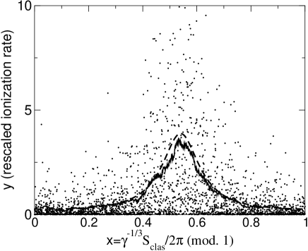
Figure 8: Rescaled ionization rates $y_{n}$, eq. (16), of the $m=0$ series for $f=0.0025$ and $\epsilon=-0.1005$, as a function of $x,$ eq. (21). $x$ represents (within a multiplicative $2\pi$ factor), the phase accumulated by the wavefunction along the periodic orbit in the inner potential well. There are large fluctuations, as expected in a chaotic system, but the average behavior is obviously dependent on $x,$ which proves that the periodic orbit strongly affects the width. A pure Random Matrix approach predicts a uniform distribution independent of $x$. The solid line is a running average which smoothes the fluctuations and clearly shows the resonant behavior of the average width with $x$. The dashed line is the semiclassical prediction, eq. (23), which incorporates the effect of the periodic orbit.

The last step is to characterize precisely the fluctuations of the individual widths that appear on top of the global exponential decrease and the modulations discussed above. Such fluctuations are thought to be unavoidable in a chaotic system, and are even a signature of the presence of chaos. In a semiclassical point of view, they can be seen as the effect of the whole set of (unstable) periodic orbits in the inner potential well. Each orbit approaching the saddle point contributes an oscillatory term analogous to eq. (4) to the width and the individual widths are just the result of the superposition of plenty of such terms which oscillate rapidly: it results in apparently random fluctuations around the mean value. A number of peaks are visible in the Fourier transformed spectra in Fig. 6; semiclassical theory tells us that they appear at the actions of periodic orbits. In our specific case, it is visible that most of them are clustered at actions slightly smaller than the action of the $z$ orbit and its repetitions. Physically, they correspond to orbits mainly located close to the $z$ axis, born from the $z$ orbit at the bifurcations discussed above. There is actually a very large number of such orbits with similar shapes, but differing by small details. Thus, it is in general difficult to associate a peak in the Fourier transform with a single periodic orbit. Except for the lowest members, we could not assign unambiguously such peaks. This is not a simple problem: indeed, many orbits are very close in phase space and, for a finite value of $\hbar_{\mathrm{eff}},$ cannot be considered as isolated in the sense that the saddle point approximation around each orbit – a key ingredient of periodic orbit theory – is not valid. In such circumstances, it is not possible to separate the contributions of the various orbits which have to be grouped together using for example a uniform approximation mouchet99 . Note that this is a fundamental difficulty of periodic orbit theory, not a practical problem related to the proliferation of the number of orbits.

An interesting illustration of this problem may be obtained by launching a bunch of trajectories from the section $z=z_{0}$ close to the saddle point. Following the real trajectories (all started with positive momentum in $z$) until they hit again the same plane $z=z_{0}$ with positive momentum one can get a feeling of the relevant dynamics. For a fully chaotic system one could naively expect that a plot of say actions calculated along the trajectory versus the initial momentum along the $z$ axis will not show any structure. This is not true in our system as visualized in Fig. 9. Observe a strongly not ergodic behaviour with allowed actions forming almost parallel strips. A clear accumulation of actions in strips correlate nicely with peaks in the Fourier transform, Fig. 6(a), in the range just below the second repetition at $2S_{\mathrm{clas}}/2\pi=5.31$ of the straight line periodic orbit. To each strip, apart from other non-periodic trajectories, several periodic orbits contribute which slightly differ in shape (and action). As mentioned already this makes a clear association between peaks in the Fourier transform and given periodic orbits impossible.

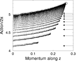
Figure 9: Distribution of actions of trajectories launched from a plane $z=z_{0}=8.82$ towards the saddle point as a function of the momentum along the $z$ axis for $m=0$, $f=0.0025$ and $\epsilon=-0.1005$. The action is calculated along a given trajectory till it hits the same plane also with positive momentum. Observe a clear structure of strips. Arrows indicate actions corresponding to peaks in the Fourier transform of the widths. The circle indicates the second repetition of the orbit along the $z$ axis with maximum action $2S_{\mathrm{clas}}/2\pi=5.31$ and momentum $p_{z}=0.2643.$

The basic assumption, usual in studies of quantum chaos, is that the effect of long periodic orbits is to create fluctuations well described by Random Matrix Theory. As – see above – the ionization rate appears as the square of some real matrix elements, the simplest hypothesis is to assume that the fluctuations are described by a Porter-Thomas distribution, eq. (17). However, the mean value $\bar{y}$ is now taken as predicted by the semiclassical theory, i.e. eq. (20). As the $x_{n}$ values are uniformly distributed, this results in a global statistical distribution:

$$P(y;R)=\int_{0}^{1}{\frac{1}{\sqrt{2\pi y\bar{y}(x)}}\exp{\left(-\frac{y}{2\bar{y}(x)}\right)}\ dx}$$ (22)

where

$$\bar{y}(x)=\frac{1-R^{2}}{1+R^{2}-2R\cos{2\pi x}}$$ (23)

This distribution is plotted in Fig. 5 as a solid line. It clearly very significantly improves over the Porter-Thomas distribution and is in excellent agreement with our numerical data. Especially, it correctly describes the excess of large ionization widths.

The same approach can be used for the data in other $m$ series. However, as is obvious in Fig. 6(b), the contribution of the $z$ orbit is much smaller in e.g. the $m=3$ series. As mentioned above, this is well understood semiclassically. In simple words, as the centrifugal term is more important, it keeps the electron away from the $z$ axis and strongly diminishes the contribution of this orbit. The $R$ parameter for the $m=3$ series can be extracted from the Fourier transform in Fig. 6(b) and is close to 0.1. The semiclassical prediction, which can be calculated in the spirit of refs. Bogomolny89 and shaw95 , is $[R(m=0)]^{4}\approx 0.12$ in reasonably good agreement. For such a small $R$ value, the deviation of the distribution (22) from Porter-Thomas is very small. This explains why the Porter-Thomas distribution correctly reproduces the results of the numerical experiment, see Fig. 4. We have also obtained results for the $m=1$ and $m=2$ series, shown in Figs. 10 and 11. Significant deviations from Porter-Thomas are observed, although smaller than for the $m=0$ series. Again, the modified distribution, eq. (22), agrees very well with the numerical results.

Figure 10: Same as figures 4 and 5, but for the $m=1$ series. The effect of scarring is intermediate and some deviations from the Porter-Thomas (Random Matrix Theory) distribution (dashed line) are observed. In contrast, the agreement with the model taken into account the scarring by the $z$ orbit, eq. (22) and solid line, is much better.

Figure 11: Same as figures 4 and 5, but for the $m=2$ series. The effect of scarring is small and only marginal deviations from the Porter-Thomas (Random Matrix Theory) distribution (dashed line) are observed.

An alternative approach to the statistical properties of the ionization widths is possible. From the semiclassical approach, we know both the average trend and the modulations; we can thus subtract (or rather divide) these factors out in order to concentrate on the fluctuations. We thus rescale the numerical data to the expected average+oscillatory behavior, that is define:

$$z_{n}=\frac{y_{n}}{\bar{y}(\hbar_{n})}$$ (24)

with $\bar{y}$ is defined in eq. (20).

The statistical distribution of the $z$ variable is shown in Fig. 12, for the $m=0$ series. As can be seen, it agrees very well with a pure Porter-Thomas distribution. This fully confirms that, once the average and oscillatory behavior have been properly taken into account, only the standard fluctuations described by Random Matrix Theory persist.

Figure 12: Statistical distribution of the ionization widths, rescaled according to eq. (24), to take into account tunneling and the effect of the periodic orbit along the field axis. A good agreement is obtained with the Porter-Thomas distribution, eq. (17), shown as a dashed line. The data are the same as in Fig. 5. The fact that a good agreement is obtained indicates that our model describes scarring and tunneling in a satisfactory manner.

Finally, we have studied a slightly less realistic system: the two-dimensional hydrogen atom in parallel electric and magnetic fields, obtained from the previous system by imposing that the motion takes place in the $(x,z)$ plane. The classical dynamics is exactly the same than for $m=0$ states (obviously the motion is planar for such cases). One could thus naively expect the same properties for the ionization widths for the quantum system. This is however not entirely true for two reasons:

• The zero-point transverse motion is now in one dimension instead of two. Thus, the shift energy is reduced by a factor 2 compared to eq. (10):

  $$\epsilon_{2D}=\frac{1}{4}\gamma^{1/3}=\frac{1}{4}\hbar_{\mathrm{eff}}.$$ (25)

  The modified scaled energy, eq. (13), must be modified accordingly.

• The stability matrix is a $2\times 2$ matrix instead of a $4\times 4$ matrix. As explained in the appendix, this results in a denominators in eqs. (1)-(4), to be square roots of the three-dimensional results for $m=0.$

The net effect is that the instability of the real orbit in the potential well is significantly reduced, simply because there is less space for the electron to escape far from the $z$ axis. The analysis is similar to the three-dimensional $m=0$ case, with the parameter $R$ being now taken at power 1/2, i.e. $R\approx 0.77$ instead of $R\approx 0.59.$ Stronger deviations from the Porter-Thomas distribution are thus expected for the $y_{n}.$ Figs. 13 and 14 show that it is indeed the case. Once more, the agreement with the modified Porter-Thomas distribution, eq. (22) is very good.

Figure 13: Same as figures 4 and 5, but for the two-dimensional hydrogen atom in parallel electric and magnetic fields. Because of the reduced dimensionality, the motion transverse to the $z$ periodic orbit is less unstable than in the three-dimensional atom, and the effect of scarring is enhanced. Very large deviations from the Porter-Thomas (Random Matrix Theory) distribution (dashed line) are observed, but the improved model, eq. (22) (solid line), reproduces well the numerical results.

Figure 14: Same as Fig. 12, for the two-dimensional model of the atom in parallel electric and magnetic fields (data as in Fig. 13). Again, scarring is well accounted for by our model.

VII Conclusion

In this paper, we have studied the widths (ionization rates) of resonances of a realistic system, the hydrogen atom in parallel electric and magnetic fields, in conditions where the classical dynamics is chaotic. We have shown that, using a semiclassical approach without any adjustable parameter but only with classical ingredients, we are able to predict analytically the average behavior of the widths. We have also shown the existence of a modulation of the average width associated with a periodic orbit and calculated quantitatively its properties, again using only classical ingredients. Finally, the residual fluctuations have been shown to be accurately described by a Random Matrix Model. This proves that a proper combination of semiclassics and Random Matrix Theory can predict the behavior of the system vs. ionization.

Our results are comparable to the ones obtained on a model system in creagh02 . For example, their Fig. 1 is clearly comparable to our Fig. 8. Note however that, due to the specificities of our realistic system, the expressions we obtain have a simpler form. On a different model system, Bies et al. bies01 observed also deviations from the Porter-Thomas distribution. Part of the deviation is due to the relatively small value of the effective Planck constant, but another part is certainly due to scarring. Their Figs. 4 and 5 are again very comparable to our Fig. 8. Because they do not consider a scaling system, the classical dynamics – and consequently the properties of the periodic orbits – change with energy which makes a comparison with our distribution rather difficult. We however have little doubt that the basic process at work is similar to ours.

VIII Acknowledgments

We are grateful to Niall Whelan and Stephen Creagh for an initial stimulation to look at tunneling in parallel fields problem. We thank W.E. Bies, L. Kaplan and E.J. Heller for permission to use their data for our manipulations. Support of KBN under project 5P03B-08821 (JZ) is acknowledged. The additional support of the bilateral Polonium and PICS programs is appreciated. Laboratoire Kastler Brossel de l’Université Pierre et Marie Curie et de l’Ecole Normale Supérieure is UMR 8552 du CNRS. CPU time on various computers has been provided by IDRIS.

*

Appendix A Classical dynamics near the saddle point

In this appendix, we discuss how the various classical quantities which enter the semiclassical formula can be calculated in our specific system, the hydrogen atom in parallel electric and magnetic fields.

The Hamiltonian of the system is given, in scaled units, by eq. (6). The saddle point is located along the $z$ axis at position:

$$z_{\mathrm{saddle}}=\frac{1}{\sqrt{f}},$$ (26)

with energy $\epsilon_{\mathrm{ion}}=-2\sqrt{f}.$

As we are interested in highly excited states lying in the immediate vicinity of the saddle point energy, it is convenient to expand the Hamiltonian at second order around the saddle point. The normal modes of this harmonic approximation are along the $z$ axis and in the $x-y$ plane. In the $x-y$ plane, the saddle point is a potential minimum associated with a vibration frequency:

$$\omega_{\rho}=\frac{\sqrt{1+4f^{3/2}}}{2}.$$ (27)

Because of the azimuthal symmetry around the fields axis, this mode is degenerate. In order to have a chaotic motion in the inner potential well, the scaled energy must be large, typically of the order of -0.1, which in turns implies that $f$ is rather small. In most cases, one can thus forget the $f$ dependence in eq. (27) and use the approximation:

$$\omega_{\rho}\approx\frac{1}{2}.$$ (28)

Along the $z$ axis, the saddle point is a potential maximum. It is thus associated with an eigenmode with purely imaginary frequency $i\omega_{z}$ where:

$$\omega_{z}=\sqrt{2}f^{3/4}$$ (29)

The corresponding imaginary period is nothing, but the period of the instanton. Alternatively, $\omega_{z}$ can be viewed as the vibration frequency around the saddle point in the inverted potential. In an harmonic potential, the action of an orbit is simply (within a $2\pi$ factor) the ratio of its excitation energy (with respect to the equilibrium point) to the frequency. This yields the (imaginary) action of the instanton given by eq. (8).

The harmonic approximation around the saddle point can also be used for the calculation of the stability matrix of the instanton. Indeed, as the harmonic potential separates completely in a transverse and a longitudinal component, the monodromy matrix of the instanton in each transverse direction, after propagation during time $t,$ is simply of the form:

$$\begin{pmatrix}\cos\omega_{\rho}t&-\sin\omega_{\rho}t\\ \sin\omega_{\rho}t&\cos\omega_{\rho}t\end{pmatrix}$$ (30)

The stability matrix of the instanton is obtained by evaluating the monodromy matrix at the period of the instanton $t=2i\pi/\omega_{z}:$

$$W=\begin{pmatrix}\cosh\frac{2\pi\omega_{\rho}}{\omega_{z}}&-i\sinh\frac{2\pi\omega_{\rho}}{\omega_{z}}\\ i\sinh\frac{2\pi\omega_{\rho}}{\omega_{z}}&\cosh\frac{2\pi\omega_{\rho}}{\omega_{z}}\end{pmatrix}$$ (31)

In our case, the ratio $\omega_{\rho}/\omega_{z}$ is very large, so that the hyperbolic trigonometric functions can be approximated by an exponential, yielding:

$$\sqrt{-\mathrm{det}(W-I)}\approx\exp{\left(\frac{\pi\omega_{\rho}}{\omega_{z}}\right)}$$ (32)

For the three-dimensional hydrogen atom, the stability matrix is a $4\times 4$ matrix which actually splits in two $2\times 2$ identical blocks (along the $x$ and $y$ directions) of type (31). Thus, the contribution (32) must be squared to get the correct semiclassical contribution. In contrast, for the simplified two-dimensional model, there is only one such contribution.

If one uses the approximate value (28) in eq. (32), one finally gets the contribution (9).

The last ingredient in the semiclassical approximation is the stability matrix of the real periodic orbit in the inner potential well. As explained in the main text, the series of bifurcations taking place in the vicinity of the saddle point energy implies that this matrix changes rapidly with $\epsilon.$ On the other hand, when $\epsilon$ is varied, the dynamics inside the potential well is only weakly affected: the main effect is that the electron spends less or more time in the immediate vicinity on the saddle point. As the transverse potential is there rather steep, the stability matrix varies a lot. These modifications are essentially described by a multiplication by a matrix similar to (30). A small variation of the period of the orbit is enough to affect strongly the matrix. However, it is the product of the stability matrices of the instanton and the real periodic orbit which describes the semiclassical contribution, eq. (4). As it is the very same matrix type (30) which contributes to the two stability matrix, it turns out that the modulus of $\det(WM-I)$ actually depends weakly on $\epsilon$ as shown in Fig. 7.

References

- (1) O. Bohigas, in Chaos and Quantum Physics, 1989 Les Houches Lecture Session LII, edited by M. J. Giannoni, A. Voros, and J. Zinn-Justin (North-Holland, Amsterdam, 1991), p. 87.
- (2) F. Haake, Quantum Signatures of Chaos, Vol. 54 of Springer Series in Synergetics (Springer, Berlin, 1991).
- (3) P. Gaspard, Chaos, Scattering and Statistical Mechanics (Cambridge University Press, Cambridge, 1998).
- (4) M. Brack and R. K. Bhaduri, Semiclassical Physics (Addison-Wesley, Reading, 1997).
- (5) H. J. Stöckmann, Quantum Chaos: An Introduction (Cambridge University Press, Cambridge, 1999).
- (6) O. Bohigas, S. Tomsovic, and D. Ullmo, Phys. Rev. Lett. 64, 1479 (1990).
- (7) O. Bohigas, S. Tomsovic, and D. Ullmo, Phys. Rep. 223, 43 (1993).
- (8) S. Tomsovic and D. Ullmo, Phys. Rev. E50, 145 (1994).
- (9) V. Averbukh, N. Moiseyev, B. Mirbach, and H. J. Korsch, Z. Phys. D 35, 247 (1995).
- (10) F. Leyvraz and D. Ullmo, J. Phys. A 29, 2529 (1996).
- (11) J. Zakrzewski, D. Delande, and A. Buchleitner, Phys. Rev. E57, 1458 (1998).
- (12) J. Zakrzewski, D. Delande, and A. Buchleitner, Acta Physica Polon. A 93, 179 (1998).
- (13) S. D. Frischat and E. Doron, Phys. Rev. E57, 1421 (1998).
- (14) C. Dembowski et al., Phys. Rev. Lett. 84, 867 (2000).
- (15) A. Mouchet and D. Delande, Phys. Rev. E67, 046216 (2003).
- (16) T. A. Brody et al., Rev. Mod. Phys. 53, 385 (1981).
- (17) M. L. Mehta, Random Matrices (Academic Press, San Diego, 1991).
- (18) R. A. Jalabert, A. D. Stone, and Y. Alhassid, Phys. Rev. Lett. 68, 3468 (1992).
- (19) H. Nakamura and S. Kato, J. Chem. Phys. 112, 1785 (2000).
- (20) S. C. Creagh and N. D. Whelan, Phys. Rev. Lett. 77, 4975 (1996).
- (21) S. C. Creagh and N. D. Whelan, Ann. Phys. 272, 196 (1999).
- (22) S. C. Creagh and N. D. Whelan, Phys. Rev. Lett. 82, 5237 (1999).
- (23) S. Creagh, S.-Y. Lee, and N. Whelan, Ann. Phys. 295, 194 (2002).
- (24) A. Shudo and K. S. Ikeda, Phys. Rev. Lett. 74, 682 (1995).
- (25) A. Shudo and K. S. Ikeda, Physica D 115, 234 (1998).
- (26) S. C. Creagh and N. D. Whelan, Phys. Rev. Lett. 84, 4084 (2000).
- (27) E. J. Heller, in Classical and Quantum Chaos, edited by A. Voros, M. Giannoni, and A. Zinn-Justin (Elsevier, Amsterdam, 1991), Chap. Scars.
- (28) E. B. Bogomolny, Physica D 31, 169 (1988).
- (29) L. Kaplan, Phys. Rev. Lett. 80, 2582 (1998).
- (30) L. Kaplan, Phys. Rev. Lett. 81, 3371 (1998).
- (31) W.E. Bies, L. Kaplan, and E.J. Heller, Phys. Rev. E64, 016204 (2001).
- (32) O. Brodier, P. Schlagheck, and D. Ullmo, Ann. Phys. 300, 88 (2002).
- (33) P. Cacciani et al., Phys. Rev. Lett. 56, 1467 (1986).
- (34) R.L. Waterland, J.B. Delos, and M.L. Du, Phys. Rev. A35, 5064 (1987).
- (35) D. Delande, in Chaos et Physique Quantique—Chaos and Quantum Physics, Les Houches, école d’été de physique théorique 1989, session LII, edited by M. Giannoni, A. Voros, and J. Zinn-Justin (North-Holland, Amsterdam, 1989), pp. 665–726.
- (36) H. Friedrich and D. Wintgen, Phys. Rep. 183, 37 (1989).
- (37) B. Grémaud, D. Delande, and J. C. Gay, Phys. Rev. Lett. 70, 1615 (1993).
- (38) K. Dupret, J. Zakrzewski, and D. Delande, Europhys. Lett. 31, 251 (1995).
- (39) W. P. Reinhardt, Annu. Rev. Phys. Chem. 33, 323 (1982).
- (40) A. Maquet, S.-I. Chu, and W. P. Reinhardt, Phys. Rev. 27, 2946 (1983).
- (41) Y. K. Ho, Phys. Rep. 99, 1 (1983).
- (42) D. Delande and J.-C. Gay, J. Phys. B: Atom. Mol. Opt. Phys.19, 173 (1986).
- (43) C. Lanczos, J. Res. Nat. Bur. Standards, Sect B 45, 225 (1950).
- (44) E. B. Bogomolny, JETP Lett. 47, 526 (1988).
- (45) E. B. Bogomolny, JETP 69, 275 (1989).
- (46) J.A. Shaw, J.B. Delos, M. Courtney, and D. Kleppner, Phys. Rev. A52, 3695 (1995).
- (47) J. Zakrzewski, D. Delande, and A. Buchleitner, Phys. Rev. Lett. 75, 4015 (1995).
- (48) W. Press, S. Teukolsky, W. Vetterling, and B. Flannery, Numerical Recipes in Fortran (Cambridge University Press, Cambridge, 1992).
- (49) C. Porter and R. Thomas, Phys. Rev. 104, 483 (1956).
- (50) M. Brack, Foundations of Physics 31, 209 (2001).
- (51) D. Wintgen, J. Phys. B: Atom. Mol. Opt. Phys.20, L511 (1987).
- (52) P. Leboeuf and A. Mouchet, Ann. Phys. 275, 54 (1999).