Drag Reduction by Polymers in Wall Bounded Turbulence

Abstract

We address the mechanism of drag reduction by polymers in turbulent wall bounded flows. On the basis of the equations of fluid mechanics we present a quantitative derivation of the “maximum drag reduction (MDR) asymptote” which is the maximum drag reduction attained by polymers. Based on Newtonian information only we prove the existence of drag reduction, and with one experimental parameter we reach a quantitative agreement with the experimental measurements.

The addition of few tens of parts per million (by weight) of long-chain polymers to turbulent fluid flows in channels or pipes can bring about a reduction of the friction drag by up to 80% 49Toms ; 75Vir ; 97VSW ; 00SW . This phenomenon of “drag reduction” is well documented and is used in technological applications from fire engines (allowing a water jet to reach high floors) to oil pipes. In spite of a large amount of experimental and simulational data, the fundamental mechanism has remained under debate for a long time 69Lu ; 90Ge ; 00SW . In such wall-bounded turbulence, the drag is caused by momentum dissipation at the walls. For Newtonian flows (in which the kinematic viscosity is constant) the momentum flux is dominated by the so-called Reynolds stress, leading to a logarithmic (von-Karman) dependence of the mean velocity on the distance from the wall 00Pope . However, with polymers, the drag reduction entails a change in the von-Karman log law such that a much higher mean velocity is achieved. In particular, for high concentrations of polymers, a regime of maximum drag reduction is attained (the “MDR asymptote”), independent of the chemical identity of the polymer 75Vir , see Fig. 1.

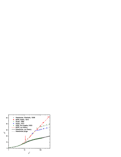
Figure 1: Mean normalized velocity profiles as a function of the normalized distance from the wall during drag reduction. The data points from numerical simulations (green circles) 03ACLPP and the experimental points (open circles) 99WMH represent the Newtonian results. The black solid line is our theory Eq.(13), which for large $y^{+}$ agrees with von-Karman’s logarithmic law of the wall (2). The red data points (squares) 72RS represent the Maximum Drag Reduction (MDR) asymptote. The dashed red curve represents our theory for the profile (Drag Reduction by Polymers in Wall Bounded Turbulence) which for large $y^{+}$ agrees with the universal law (16). The arrow marks the crossover from the viscous linear law (12) to the asymptotic logarithmic law (16). The blue filled triangles 72RS and green open triangles 69Rud represent the cross over, for intermediate concentrations of the polymer, from the MDR asymptote to the Newtonian plug. Our theory is not detailed enough to capture this cross over properly.

In this Letter we elucidate the fundamental mechanism for this phenomenon: while momentum is produced at a fixed rate by the forcing, polymer stretching results in a suppression of the momentum flux from the bulk to the wall. Accordingly the mean velocity in the channel must increase. We derive a new logarithmic law for the mean velocity with a slope that fits existing numerical and experimental data. The law is universal, thus explaining the MDR asymptote.

Turbulent flows in a channel are conveniently discussed 00Pope for fixed pressure gradients $p^{\prime}\equiv-\partial p/\partial x$ where $x$, $y$ and $z$ are the lengthwise, wall-normal and spanwise directions respectively. The length and width of the channel are usually taken much larger than the mid-channel height $L$, making the latter a natural re-scaling length for the introduction of dimensionless (similarity) variables. Thus the Reynolds number ${{\mathcal{R}}}\mkern-3.1mue$, the normalized distance from the wall $y^{+}$ and the normalized mean velocity $V^{+}(y^{+})$ (which is in the $x$ direction with a dependence on $y$ only) are defined by

$${{\mathcal{R}}}\mkern-3.1mue\equiv{L\sqrt{\mathstrut p^{\prime}L}}/{\nu_{0}}\ ,\ y^{+}\equiv{y{{\mathcal{R}}}\mkern-3.1mue}/{L}\ ,\ V^{+}\equiv{V}/{\sqrt{\mathstrut p^{\prime}L}}\ ,$$ (1)

where $\nu_{0}$ is the kinematic viscosity. One of the most famous universal aspects of Newtonian turbulent channel flows is the “logarithmic law of the wall” which in these coordinates is expressed as

$$V^{+}(y^{+})=\kappa_{{}_{\text{K}}}^{-1}\ln y^{+}+B\,,\quad{\rm for}~{}y^{+}\gtrsim 30\,,$$ (2)

where the von-Karman constant $\kappa_{{}_{\text{K}}}\approx 0.436$ and intercept $B\approx 6.13$ 97ZS . For $y^{+}<10$ one observes a viscous sub-layer, $V^{+}(y^{+})=y^{+}$, Fig. 1. The riddle of drag reduction is then introduced in relation to this universal law: in the presence of long chain polymers the mean velocity profile $V^{+}(y^{+})$ (for a fixed value of $p^{\prime}$ and channel geometry) changes dramatically. For sufficiently large concentration of polymers $V^{+}(y^{+})$ saturates to a new (universal, polymer independent) “law of the wall” 75Vir ,

$$V^{+}(y^{+})=11.7\ln y^{+}-17\,,\quad{\rm for}~{}y^{+}\gtrsim 12\ .$$ (3)

For smaller concentration of polymers the situation is as shown in Fig. 1. The Newtonian law of the wall (2) is the black solid line for $y^{+}\gtrsim 30$. The MDR asymptote (3) is the dashed red line. For intermediate concentrations the mean velocity profile starts along the asymptotic law (3), and then crosses over to the so called “Newtonian plug” with a Newtonian logarithmic slope identical to the inverse of von-Karman’s constant. The region of values of $y^{+}$ in which the asymptotic law (3) prevails was termed “the elastic sub-layer” 75Vir . The relative increase of the mean velocity (for a given $p^{\prime}$) due to the existence of the new law of the wall (3) is the phenomenon of drag reduction. Thus the main theoretical challenge is to understand the origin of the new law (3), and in particular its universality, or independence of the polymer used. A secondary challenge is to understand the concentration dependent cross over back to the Newtonian plug. In this Letter we argue that the phenomenon can be understood mainly by the influence of the polymer stretching on the $y^{+}$-dependent effective viscosity. The latter becomes a crucial agent in carrying the momentum flux from the bulk of the channel to the walls (where the momentum is dissipated by friction). In the Newtonian case the viscosity has a negligible role in carrying the momentum flux; this difference gives rise to the change of Eq. (2) in favor of Eq. (3) which we derive below.

The equations of motion of polymer solutions can be written as 87BCAH ; 94BE :

$${\partial{\bm{U}}}/{\partial t}+{\bm{U}}\cdot{\bm{\nabla}}{\bm{U}}=-{\bm{\nabla}}p+{\bm{\nabla}}\cdot{\bm{{\cal T}}}+\nu_{0}\nabla^{2}{\bm{U}}\ ,$$ (4)

where ${\bm{{\cal T}}}$ is the extra stress tensor that is due to the polymer. Denoting the polymer end-to-end vector distance (normalized by its equilibrium value) as ${\bm{r}}$, the average dimensionless extension tensor ${\bm{{\cal R}}}$ is ${\cal R}_{ij}\equiv\langle r_{i}r_{j}\rangle$, and the extra stress tensor is (with $\omega_{ij}\equiv\partial U_{i}/\partial x_{j}$),

$${\bm{{\cal T}}}=\nu_{p}\left({\bm{\omega}}\cdot{\bm{{\cal R}}}+{\bm{{\cal R}}}\cdot{\bm{\omega}}^{T}-{\partial{\bm{{\cal R}}}}/{\partial t}-{\bm{U}}\cdot{\bm{\nabla}}{\bm{{\cal R}}}\right)\ .$$ (5)

Here $\nu_{p}$ (proportional to the polymer concentration) is the polymeric contribution to the viscosity in the limit of zero shear. In order to develop a transparent theory we propose to ignore the fluctuations of ${\bm{{\cal R}}}$ compared to its mean. In other words, we will take ${\bm{{\cal R}}}\approx\langle{\bm{{\cal R}}}\rangle$. Simplifying further the tensor structure, assuming that ${\cal R}_{ij}={\cal R}\delta_{ij}$ we can rewrite Eq. (4) in the form

$${\partial U_{i}}/{\partial t}+U_{j}\nabla_{j}U_{i}=-\nabla_{i}P+\nabla_{j}\nu\,(\omega_{ij}+\omega_{ji})\ ,$$ (6)

$$\nu=\nu_{0}+\nu_{p}{{\cal R}}\ ,\quad P=p+{\partial\nu}/{\partial t}+{\bm{U}}\cdot{\bm{\nabla}}\nu\ ,$$ (7)

with a scalar ($y$-dependent) effective viscosity $\nu$.

Armed with the effective equation we establish the mechanism of drag reduction following the standard strategy of Reynolds, considering the fluid velocity ${\bm{U}}({\bm{r}})$ as a sum of its average (over time) and a fluctuating part:

$${\bm{U}}({\bm{r}},t)={\bm{V}}(y)+{\bm{u}}({\bm{r}},t)\ ,\quad{\bm{V}}(y)\equiv\langle{\bm{U}}({\bm{r}},t)\rangle\ .$$ (8)

For a channel of large length and width all the averages, and in particular ${\bm{V}}(y)\Rightarrow V(y)$, are functions of $y$ only. The objects that enter the theory are the mean shear $S(y)$, the Reynolds stress $W(y)$ and the kinetic energy $K(y)$; these are defined respectively as

$$S(y)\equiv dV(y)/dy\ ,\ W(y)\equiv-\langle u_{x}u_{y}\rangle\ ,\ K(y)=\langle|{\bm{u}}|^{2}\rangle/2.$$

A well known exact relation 00Pope between these objects is the point-wise balance equation for the flux of mechanical momentum; near the wall (for $y\ll L$) it reads :

$$\nu(y)S(y)+W(y)=p^{\prime}L\ .$$ (9)

On the RHS of this equation we see the production of momentum flux due to the pressure gradient; on the LHS we have the Reynolds stress and the viscous contribution to the momentum flux, with the latter being usually negligible (in Newtonian turbulence $\nu=\nu_{0}$) everywhere except in the viscous boundary layer. The $y$ dependence of the effective viscosity $\nu(y)$ in the elastic layer will be shown to be crucial for drag reduction.

A second relation between $S(y)$, $W(y)$ and $K(y)$ is obtained from the energy balance. The energy is created by the large scale motions at a rate of $W(y)S(y)$. It is cascaded down the scales by a flux of energy, and is finally dissipated at a rate $\epsilon$, where $\epsilon=\nu\langle\omega^{2}_{ij}\rangle$. We cannot calculate $\epsilon$ exactly, but we can estimate it rather well at a point $y$ away from the wall. When viscous effects are dominant, this term is estimated as $\nu(a/y)^{2}K(y)$ (the velocity is then rather smooth, the gradient exists and can be estimated by the typical velocity at $y$ over the distance from the wall). Here $a$ is a constant of the order of unity. When the Reynolds number is large, the viscous dissipation is the same as the turbulent energy flux down the scales, which can be estimated as $K(y)/\tau(y)$ where $\tau(y)$ is the typical eddy turn over time at $y$. The latter is estimated as $y/b\sqrt{K(y)}$ where $b$ is another constant of the order of unity. We can thus write the balance equation at point $y$ as

$$\nu(y)({a}/{y})^{2}K(y)+{b\,{K^{3/2}(y)}}/y=W(y)S(y)\,,$$ (10)

where the bigger of the two terms on the LHS should win. We note that contrary to Eq. (9) which is exact, Eq.(10) is not exact. We expect it however to yield good order of magnitude estimates as is demonstrated below. Finally, we quote the experimental fact 75Vir ; 01PNVH that outside the viscous boundary layer

$$\frac{W(y)}{K(y)}=\Bigg{\{}\begin{array}[]{ll}c_{{}_{\text{N}}}^{2}\,,&\text{for Newtonian flow,}\\ &\\ c_{{}_{\text{V}}}^{2}\,,&\text{for viscoelastic flow.}\\ \end{array}$$ (11)

The coefficients $c_{{}_{\text{N}}}$ and $c_{{}_{\text{V}}}$ are bounded from above by unity. (The proof is $|c|\equiv|W|/K\leq 2|\langle u_{x}u_{y}\rangle|/\langle u_{x}^{2}+u_{y}^{2}\rangle\leq 1$, because $(u_{x}\pm u_{y})^{2}\geq 0$). While $c_{{}_{\text{N}}}$ is known quite accurately, $c_{{}_{\text{N}}}\approx 0.5$, the actual values of $c_{{}_{\text{V}}}$ varies somewhat from experiment to experiment, such that the ratio $c_{{}_{\text{V}}}/c_{{}_{\text{N}}}$ (which is all that we need to use below) varies between 0.3 and 0.7. In our estimates we take $c_{{}_{\text{V}}}/c_{{}_{\text{N}}}=0.5$.

We show now that Eqs. (9 – 11) are sufficient for deriving the Newtonian law (2) and the viscoelastic law (3) with equal ease. Begin with the Newtonian case. The result of this derivation is not new - but we want to stress that the same equations give rise to both the well known and the new results. Substitute Eq. (11) in Eqs. (9, 10) with $\nu(y)=\nu_{0}$, turning them into algebraic equations for $K(y)$ and $S(y)$, and eventually to a first order differential equation for $V(y)$. In the viscous sub-layer $K(y)=0$, and the solution in re-scaled coordinates is

$$V^{+}(y^{+})=y^{+}\ ,\quad y^{+}\leq y^{+}_{v}\equiv a/c_{{}_{\text{N}}}\ ,$$ (12)

Outside the viscous sub-layer ($y^{+}>y^{+}_{v}$) we find

$$V^{+}(y^{+})=\kappa_{{}_{\text{K}}}^{-1}\ln Y(y^{+})+B-\Delta(y^{+})\,,$$ (13a)

$$B=2y^{+}_{v}-\kappa_{{}_{\text{K}}}^{-1}\ln\left[{e\,(1+2\,\kappa_{{}_{\text{K}}}y^{+}_{v})}/{4\kappa_{{}_{\text{K}}}}\right]\,,$$ (13b)

where $\kappa_{{}_{\text{K}}}=c_{{}_{\text{N}}}/b$ and we defined

$$Y(y^{+}) = \Big{[}y^{+}+\sqrt{{y^{+}}^{2}-{y_{v}^{+}}^{2}+\big{(}2\kappa_{{}_{\text{K}}}\big{)}^{-2}}\Big{]}\Big{/}2\,,$$

$$\Delta(y^{+}) = \frac{2\,\kappa_{{}_{\text{K}}}^{2}{y_{v}^{+}}^{2}+4\kappa_{{}_{\text{K}}}\big{[}Y(y^{+})-y^{+}\big{]}+1}{2\kappa_{{}_{\text{K}}}^{2}y^{+}}\ .$$

For $y^{+}\gg y^{+}_{v}$ Eqs. (13) turns into (2) since $Y(y^{+})\to y^{+}$ and $\Delta(y^{+})\to 0$.

Note that Eqs (13) pertain to the whole $y^{+}$ domain. By taking the experimental values of $\kappa_{{}_{\text{K}}}$ and $B$ we compute $y^{+}_{v}\approx 5.6$ to be compared with the experimental value of 5.5$\pm 0.5$, cf. 00Pope . The resulting Newtonian profile, Eqs. (12) and (13), is shown in Fig. 1 as the black solid line. The excellent agreement with the experimental and numerical data in the entire region of $y^{+}$ indicates that our balance equations are sufficiently accurate and we can proceed to the viscoelastic case.

To see how the law (3) emerges we consider Eqs. (9) and (10) with $y$-dependent effective viscosity. We should warn the reader that this is not fully justified – there are terms in the full viscoelastic equations which cannot be simplified to the form of a space dependent viscosity. Nevertheless we propose (and justify further below) that the terms with effective viscosity are the main terms that allow the momentum flux to be carried in the elastic sublayer. In other words, when the concentration of the polymer is large enough we can neglect the second term in favor of the first in Eq. (9) and estimate $\nu(y)=Lp^{\prime}/S(y)$. Substituting this estimate in Eq. (10), neglecting the second term on the LHS, using Eq. (11), and finally re-scaling the variables results in

$${\partial V^{+}}/{\partial y^{+}}={c_{{}_{\text{N}}}}{y^{+}_{v}}/{c_{{}_{\text{V}}}}{y^{+}}\ .$$ (14)

From here follows immediately the new “logarithmic law of the wall”

$$V^{+}(y^{+})={\kappa_{{}_{\text{V}}}}^{-1}\ln y^{+}+B_{{}_{\text{V}}}\,,\quad\kappa_{{}_{\text{V}}}={c_{{}_{\text{V}}}}/{c_{{}_{\text{N}}}}{y^{+}_{v}}\,,$$ (15)

where the intercept $B_{{}_{\text{V}}}$ is still unknown (but will be determined momentarily). The slope of the new law is independent of the polymer concentration and is greater than the von-Karman slope $1/\kappa_{{}_{\text{K}}}$; the ratio of the slopes is in fact $\kappa_{{}_{\text{K}}}y^{+}_{v}c_{{}_{\text{N}}}/c_{{}_{\text{V}}}$, which is about 4.9 according to the above estimates $c_{{}_{\text{N}}}/c_{{}_{\text{V}}}\approx 0.5$ and $y^{+}\approx 5.6$. Comparing with the measured ratio of slopes in Eqs. (2) and (3) which is about 5.1, we consider our estimates to be quite on the mark. As said before, this increase in slope is the phenomenon of drag reduction. We stress that the information gained from the Newtonian data alone is sufficient to predict drag reduction, since $c_{{}_{\text{V}}}\leq 1$.

To find $B_{{}_{\text{V}}}$ we match the logarithmic law (15) to the viscous sublayer solution (12) by the value of $V^{+}(y^{+})$ and its derivative. First, the logarithmic law has slope 1 at $y^{+}_{m}=\kappa_{{}_{\text{V}}}^{-1}$. Next, matching at this point the viscous solution $V^{+}(y^{+}_{m})=\kappa_{{}_{\text{V}}}^{-1}$ to (15) we find $B_{{}_{\text{V}}}=\ln(e\,\kappa_{{}_{\text{V}}})/\kappa_{{}_{\text{V}}}$. We note that if we substitute the experimental value $\kappa_{{}_{\text{K}}}^{-1}=11.7$ we find $B_{{}_{\text{V}}}=-17$ in perfect agreement with Eq. (3). We thus write the law (15) in its final form (with just one constant remaining)

$$V^{+}(y^{+})=\frac{1}{\kappa_{{}_{\text{V}}}}\ln\left(e\,\kappa_{{}_{\text{V}}}\,y^{+}\right)\ .$$ (16)

Note that this universal result is obtained without reference to any model of the polymer dynamics, and the only assumptions are that the polymer viscosity dominates the momentum transfer in the elastic layer and the logarithmic law (15) is valid all the way to $y^{+}_{m}$. At this point we demonstrate that these two assumptions, which lead to the universality of (16), are well supported by a closer consideration of the polymer dynamics.

The fundamental reason for the appearance of a $y$-dependent viscosity is the coil-stretch transition of the polymers under turbulent shear. This transition occurs in any reasonable model of the polymer-turbulence interaction, the simplest of which is of the form 77BAH

$${d{\cal R}}/{dt}=-{{\cal R}}/{\tilde{\tau}_{p}}+s(y){\cal R}\ ,\quad s(y)\equiv\sqrt{\langle\omega_{ij}^{2}\rangle}\ ,$$ (17)

where $\tilde{\tau}_{p}$ is the polymer relaxation time. In the elastic sublayer we estimate $s(y)=g\sqrt{K(y)}/y$, with some constant $g\approx O(1)$, and expect a coil stretch transition when $g\sqrt{K(y)}/y=1/\tilde{\tau}_{p}$. Defining $\tau_{p}\equiv g\tilde{\tau}_{p}$ we then find in the elastic sublayer (where polymers are stretched)

$$K(y)=\left(y/\tau_{p}\right)^{2}\ .$$ (18)

This equation is important since it can be solved together with Eqs. (9) and (10) to find $S^{+}(y^{+})$ when the polymers are stretched. The answer is

$$S^{+}(y^{+}) = \frac{1}{\kappa_{{}_{\text{V}}}y^{+}}\Big{\{}\Big{(}\frac{y^{+}L}{{{\mathcal{R}}}\mkern-3.1mue\,\ell}\Big{)}$$

$$+\sqrt{1+\big{[}\big{(}2\kappa_{{}_{\text{K}}}y_{v}^{+}c_{{}_{\text{V}}}\big{)}^{2}-1\big{]}\Big{(}\frac{y^{+}L}{{{\mathcal{R}}}\mkern-3.1mue\,\ell}\Big{)}^{2}}\Big{\}}\,,$$

where $\ell=2\,\kappa_{{}_{\text{K}}}y^{+}_{v}c_{{}_{\text{V}}}\tau_{p}\sqrt{Lp^{\prime}}$. Equation (14) is recaptured from this, more general equation, when ${{\mathcal{R}}}\mkern-3.1mue$  is large and $\{\dots\}\to 1$. Then the identity of the polymer is lost, giving rise to the universal drag reduction asymptote (16). It can be also checked that the matching point $y^{+}_{m}$ used above indeed connects smoothly the viscous sublayer to the asymptotic law (16) (see arrow in Fig. 1). We can therefore conclude that our derivation of Eq. (16) is fully consistent with the polymer dynamics, and we understand how the polymer characteristics drop out, leading to the universal law (16).

The mechanism of drag reduction is then the suppression of the Reynolds stress in the elastic sublayer. The Reynolds stress is the main agent for momentum flux in the Newtonian case, and its suppression results in an increase of the mean mechanical momentum (velocity) in the channel. The increase in viscosity of course leads to increased energy dissipation, but this is immaterial for the phenomenon. This is the main difference between drag reduction in wall-bounded turbulence and in homogeneous turbulence 03BDGP . We note that the theory predicts a very low value of $K(y)$ in the elastic layer. In reality in every wall bounded turbulent flows there will be ejecta of parcels of fluid with high level of $K(y)$ from the Newtonian region towards the walls. These would be picked up in measurements, and would seem to contradict the low value of $K(y)$ predicted above. In fact there is no real contradiction since such random ejecta do not contribute much to the momentum flux that is so crucial to our discussion. We also note a term in the dynamical equations for the viscoelastic flow of the form $d\langle r_{i}r_{j}\rangle/dt$, which cannot be written as an effective viscosity. This term vanishes for uncorrelated rotations of individual polymeric molecules. However it can contribute to the energy flux from the mean shear to turbulent fluctuations in wall bounded flows due to a possible “correlation instability”, which leads to synchronized rotation of neighboring polymers. A more detailed consideration of such terms should provide also the cross over behavior seen in Fig. 1.

Finally we propose direct numerical simulations in channel flows to test our approach. Instead of simulating the viscoelastic equations, we propose to simulate the Navier-Stokes equations with a space dependent viscosity according to the above theory. We predict that a viscosity profile that remains constant for $0\leq y^{+}\leq y^{+}_{{}_{\text{V}}}$, and then grows linearly towards the center, should result in drag reduction in much the same way as seen in experiments with polymers. Such simulations would render direct support to the views offered in this Letter.

References

- (1) B.A. Toms, in Proceedings of the International Congress of Rheology Amsterdam Vol 2. 0.135-141 (North Holland, 1949).
- (2) P.S. Virk, AIChE J. 21, 625 (1975)
- (3) P.S. Virk, D.C. Sherma and D.L. Wagger, AIChE Journal, 43, 3257 (1997).
- (4) K. R. Sreenivasan and C. M. White, J. Fluid Mech. 409, 149 (2000).
- (5) J. L. Lumley, Ann. Rev. Fluid Mech. 1, 367 (1969).
- (6) P.-G. de Gennes Introduction to Polymer Dynamics, (Cambridge, 1990).
- (7) S. B. Pope, Turbulent Flows (Cambridge, 2000).
- (8) R.B. Bird, C.F. Curtiss, R.C. Armstrong and O. Hassager, Dynamics of Polymeric Fluids Vol.2 (Wiley, NY 1987)
- (9) A.N. Beris and B.J. Edwards, Thermodynamics of Flowing Systems with Internal Microstructure (Oxford University Press, NY 1994).
- (10) M.V. Zagarola and A.J. Smits, Phys. Rev. Lett. 78, 239 (1997).
- (11) E. De Angelis, C.M. Casciola, V.S. L’vov, R. Piva and I. Procaccia, Phys. Rev. E., 67, 056312 (2003).
- (12) M.D. Warholic, H.Massah, T.J. Hanratty, Experiments in Fluids, 27, 461 (1999).
- (13) A. Rollin and F.A. Seyer, Can. J. Chem. Eng.,50, 714-718 (1972).
- (14) M.J. Rudd, Nature, 224, 587 (1969)
- (15) R. B. Bird, R.C. Armstorng and O. Hassager, Dynamics of Polymeric Liquids, (John Wiley, New York, 1977, Vol.2).
- (16) P.K. Ptasinski, F.T.M. Nieuwstadt, B.H.A.A. van den Brule and M.A. Hulsen, Flow, Turbulence and Combustion, 66, 159 (2001).
- (17) The importance of space dependent viscosity was already pointed out, cf. R. Govindarajan, V.S. L vov and I. Procaccia, Phys. Rev. Lett., 87, 174501 (2001).
- (18) R. Benzi, E. De Angelis, R. Govindarajan and I. Procaccia, Phys. Rev. E, in press. Also: physics/0304091