Effect of base-pair inhomogeneities on charge transport along DNA mediated by twist and radial polarons

Abstract

Some recent results for a three–dimensional, semi–classical, tight–binding model for DNA show that there are two types of polarons, named radial and twist polarons, that can transport charge along the DNA molecule. However, the existence of two types of base pairs in real DNA, makes it crucial to find out if charge transport also exist in DNA chains with different base pairs. In this paper we address this problem in its simple case, an homogeneous chain except for a single different base pair, what we call a base-pair inhomogeneity, and its effect on charge transport. Radial polarons experience either reflection or trapping. However, twist polarons are good candidates for charge transport along real DNA. This transport is also very robust with respect to weak parametric and diagonal disorder.

Keywords:DNA, polarons, charge transport
PACS: 87.-15.v,63.20.Kr,63.20.Ry,87.10.+e

1 Introduction

Charge transport in biomolecules is of relevant in many biological functions. Moveover, electronic transport plays a well known and fundamental role in many of biological processes, such as nervous conduction, photosynthesis, cellular respiration and redox reactions. Recently, DNA–mediated charge transport has focused much attention with experiments that have been conducted to determine its conductive properties, and theoretical studies have addressed the possibility of charge transport and its efficiency [1]. The importance of charge transport through DNA is significant because some mutations in living systems and radical migrations are critical issues in carcinogenesis studies and may yield insight into damage prevention or repair processes [2, 3, 4]. Moreover, charge transport has been demonstrated to proceed within HeLa cell nuclei [5] as well as in the nucleosome core particles [6], and can provide a practical method of genetic screening for known gene sequences and an alternative method to hybridization based arrays [7]. Material scientists have thought that DNA has a fundamental physical interest for the development of DNA–based molecular technologies, as it possesses ideal structural and molecular recognition properties for use in self assembling nanodevices with a definite molecular architecture [8].

Photochemical electron transfer experiments have been carried out with femtosecond resolution, and have shown, with the precise control of the DNA sequences, a fast time scale ($\leq 5$ ps) process, attributed to charge mobility along an unperturbed double strand, and a slower process ($\leq 75$ ps), that they believe reflects charge hopping between perturbed domains along the DNA strand [9].

Experimental results have explained that DNA acts as a linear chain with overlapping $\pi$ orbitals located at the stacked base pairs and its conductivity is very sensitive to disruption, caused by base–pair mistakes or interactions with proteins, in the base–pair stack. Depending on the base pair sequences the transfer can be slowed or inhibited [10].

Moreover, the robust, malleable one–dimensional structure of DNA can be used to design electronic devices based on biomaterials  [11, 12, 13, 14, 15].

The structure of the bent double helix $\lambda$-DNA can be modelled by a network of oscillators taking into account deformations of the hydrogen bonds within a base pair and twist motions between consecutive base pairs. The three–dimensional semi–classical tight–binding model for DNA that was first proposed in Ref. [16, 17] makes also the assumption that the electron motion is predominantly influenced by vibrational modes of the double helix. The nonlinear interaction between the electron and the vibrational modes is responsible of the formation of polarons or electron-vibron breathers. These are localized excitation patterns that can be static, producing charge localization, or mobile, bringing about charge transport. It has been considered some other models with inhomogeneities [18].

A variant of this model has been proposed in Ref. [19], which lifts the restriction of the previous one, that the perturbation of the spatial variables were small enough to perform a linear approximation in the dynamical equations. Two types of polarons appear depending on the parameter $\alpha$, that describes the coupling between the transfer integral and the distance between nucleotides, and the form of activation: radial polarons and twist polarons. For radial polarons, the deformations associated by the electronic charge affect mainly to the radial variables, and for twist polarons, to the angular ones. In the last case, the moving polaron is slower than in the previous one, but it is more robust with respect to the introduction of parametric disorder. See reference above for details and Ref. [20] for twist polarons in other model.

In this paper we consider the movement of polarons along DNA chains made out of different base pairs. The most simple one consists of homogeneous DNA chains except for a single different base pair, which we call base-pair inhomogeneity.

We have found that when charge transport is mediated by means of a twist polaron, this moving carrier can transport charge along a base-pair inhomogeneity in a very efficient way. Moreover, charge transport persists under the introduction of a high degree of parametric disorder, that represents the inherent disorder in the surrounding medium and the inhomogeneous distribution of counterions along the DNA duplex [21]. On the other hand, radial polarons are either reflected or trapped by the base-pair inhomogeneity, making them poor candidates for charge transport along heterogeneous DNA at least in the framework of the tight-binding models.

2 DNA model

2.1 Description

We consider a variant [19] of the model Hamiltonian for charge transport along DNA that was first proposed in  [16]. This variant consists of considering the full dynamical equations of the system instead of performing linear approximations based on the assumption that the deformations of the molecule were small.

These models were designed to implement the basic characteristics of the DNA double helix structure needed for a proper description of the charge transport dynamics. The starting point is the twist-opening model  [22, 23, 24] that has taken into account the helicoidal structure of DNA and the torsional deformations induced by the opening of the base pairs. The bases are considered as single nondeformable objects. The helicoidal structure of DNA is described in a cylindrical reference system and the n–th base pair has two degrees of freedom, namely $(r_{n},\phi_{n})$, where $r_{n}$ represents the radial displacement of the base pair from the equilibrium value $R_{0}$, and $\phi_{n}$ represents the angular deviation from equilibrium angles with respect to a fixed external reference frame. As we are interested in base pair vibrations and not in acoustic motions, the center of mass of each base pair is fixed, $i.e.$, the two bases in a base pair are constrained to move symmetrically with respect to the molecule axis. Moreover, the distances between two neighboring base pair planes will be treated as fixed, because in the axial direction DNA is less deformable than within the base pair planes [22].

A sketch of the helicoidal structure of the DNA model is shown in Fig. 1.

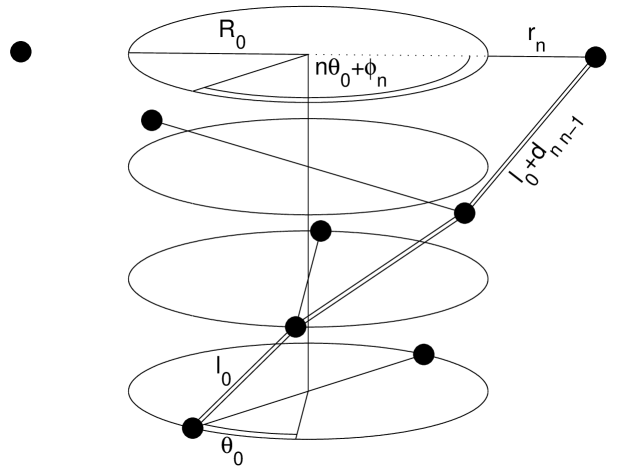
Figure 1: Sketch of the model. Filled circles represent bases. The variables used in the text are displayed.

The transversal displacements of the base pairs are deformations of the H-bonds and the angular twist and the radial vibrational motion evolve independently on two different time scales, then they can be considered as decoupled degrees of freedom in the harmonic approximation of the normal mode vibrations [25].

2.2 Hamiltonian

The Hamiltonian for the electron transport along a strand of DNA is given by $\widehat{H}=\widehat{H}_{el}+\widehat{H}_{rad}+\widehat{H}_{twist}$, where $\widehat{H}_{el}$ corresponds to the part related with the particle charge transport over the base pairs,$\widehat{H}_{rad}$ describes the dynamics of the H-bond vibrations and $\widehat{H}_{twist}$ is the part corresponding to the dynamics of the relative twist angle between two consecutive base pairs. This electronic part is described by a tight–binding system of the form:

$$\widehat{H}_{el}=\sum_{n}E_{n}|n\rangle\langle n|-V_{n-1,n}|n-1\rangle\langle n|-V_{n+1,n}|n+1\rangle\langle n|\,,$$ (1)

where $|n\rangle$ represents a localized state of the charge carrier at the $n^{th}$ base pair. The quantities $\{V_{n,n-1}\}$ are the nearest–neighbor transfer integrals along base pairs, and $\{E_{n}\}$ are the energy on–site matrix elements. A general electronic state is given by $|\Psi\rangle=\sum_{n}c_{n}(t)|n\rangle$, where $c_{n}(t)$ is the probability amplitude of finding the charged particle in the state $|n\rangle$. The time evolution of the $\{c_{n}(t)\}$ is obtained from the Schr$\ddot{o}$dinger equation $\mathrm{i}\hbar(\partial\Psi/\partial t)=\widehat{H}_{el}|\Psi\rangle$

The nucleotides are large molecules and they move much more slowly than a charged particle, then the lattice oscillators can be described classically and $\widehat{H}_{rad}$ and $\widehat{H}_{twist}$ are, de facto, classical Hamiltonians. For homogeneous chains they are given by (omitting the hat over them):

$$H_{rad} = \sum_{n}\left[\frac{1}{2M}(p^{r}_{n})^{2}+\frac{M\Omega^{2}_{r,n}}{2}r_{n}^{2}\right],$$ (2)

$$H_{twist} = \sum_{n}\left[\frac{1}{2J}(p^{\phi}_{n})^{2}+\frac{J\Omega_{\phi}^{2}}{2}\ (\phi_{n}-\phi_{n-1})^{2}\right],$$ (3)

where $p^{r}_{n}$ and $p^{\phi}_{n}$ are the conjugate momenta of the radial and angular coordinates,respectively. In these expressions $M$ is the mass of each base pair ($M=2m$,being $m$ an average estimation of the nucleotide mass), $J=M\,R_{0}^{2}$ is the moment of inertia of each base pair and $\Omega_{r,n}$ is the linear radial frequency which is proportional to the strength of the hydrogen bonds. Indeed, for an homogeneous chain all these frequencies are equals, that is, $\Omega^{2}_{r,n}=b_{n}\Omega^{2}_{r}$ with $b_{n}=1\,\forall n$.

In this paper we are interested in the study of charge transport along DNA strands where all the base pairs are of the same type, say A-T (or C-G), except only one of them which is of a different type, say C-G (or A-T). We can suppose that the ratio between the elastic constants of bonds in a C-G base pair and an A-T base pair is $3/2$ because the first involves three hydrogen bonds and the second two of them. Then, as in Ref. [26] we take $b_{n}=0.8$ for an A-T base pair, and $b_{n}=1.2$ for a C-G base pair. $\Omega_{\phi}$ is the linear twist frequency, and we represent by $\theta_{n,n-1}=(\phi_{n}-\phi_{n-1})$, the deviation of the relative angle between two adjacent base pairs from its equilibrium value $\theta_{0}$.

In general, the ionization potential of different nucleotides differs an amount of 0.2-1.0 eV [27]. In our model, this implies different values of the on site energies $E_{n}^{0}$ for each base pairs. In this work, we have focused in geometrical effects due to the stretching of the chain over the charge, and we have considered $E_{n}^{0}$ independent on the type of base.

The electronic part of the Hamiltonian, $\widehat{H}_{el}$, has a dependence on the structure variables $r_{n}$ and $\phi_{n}$ through the dependence of the matrix elements $E_{n}$ and $V_{n,n-1}$ on them. The energy on–site matrix elements are given by [28] $E_{n}=E_{n}^{0}+kr_{n}$, expressing the modulation of the on–site electronic energies $\{E_{n}^{0}\}$ by the radial deformations of the base pairs. The transfer matrix elements $V_{n,n-1}$, which are responsible for the transport of the electron along the stacked base pairs, are assumed to depend on the distances between two consecutive bases along a strand $d_{n,n-1}$ as $V_{n,n-1}=V_{0}(1-\alpha d_{n,n-1})$, where $\alpha$ is a parameter that describes the influence of the distance between nucleotides, and the later is determined by

$$d_{n,n-1} = [a^{2}+(R_{0}+r_{n})^{2}+(R_{0}+r_{n-1})^{2}-$$ (4)

$$2(R_{0}+r_{n})(R_{0}+r_{n-1})\cos(\theta_{0}+\theta_{n,n-1})]^{1/2}-l_{0},$$

with $l_{0}=(a^{2}+4R_{0}^{2}\sin^{2}(\theta_{0}/2))^{1/2},$ where $a$ is the vertical distance between two consecutive base pairs.

In this paper, as in Ref. [19], we have not used the expansion of this expression up to first order around the equilibrium positions, as was performed in Refs. [16, 17]. This allow us to consider parameters that allow larger deformations in the angular variables.

Realistic parameters for the DNA are given in Refs. [23, 29]. We have considered: $a=3.4\AA$, $m=300$ amu, $R_{0}=10\AA$,$\Omega_{r}=8\times 10^{12}$ s^-1, $\Omega_{\phi}=9\times 10^{11}$ s^-1. Ab initio calculations find that between adjacent nucleotides, the transfer integral is in order of 0.1-0.4 eV [30] . Although this transfer integral is different for each pair of different nucleotides, we will consider the same value for all neighboring cases $V_{0}=0.1$ eV, a supposition widely used and can be valid in order to reproduce ab initio results and experiments [31].

We scale the time according to $t\rightarrow\Omega_{r}t$, and we introduce the dimensionless quantities: $\tilde{r}_{n}=r_{n}\,(M\Omega_{r}^{2}/V_{0})^{1/2}$, $\tilde{k}_{n}=k_{n}/(M\Omega_{r}^{2}V_{0})^{1/2}$, $\tilde{E_{n}}=E_{n}/V_{0}$, $\tilde{\Omega}=\Omega_{\phi}/\Omega_{r}$, $\tilde{V}=V_{0}/(J\,\Omega_{r}^{2})$, $\tilde{\alpha}=\alpha\,(V_{0}/M\,\Omega_{r}^{2})^{1/2}$, $\tilde{R}_{0}=R_{0}\,(M\,\Omega_{r}^{2}/V_{0})^{1/2}$.

2.3 Dynamical equations

Using the expectation value for the electronic contribution to the Hamiltonian, the new classical Hamiltonian $\overline{H}=\langle\phi|\widehat{H}|\phi\rangle/V_{0}$ is given in the scaled variables (omitting the tildes) by

$$\overline{H} = \sum_{n}\Big{\{}\frac{1}{2}(\dot{r}_{n}^{2}+b_{n}r_{n}^{2})+\frac{R_{0}^{2}}{2}[\dot{\phi_{n}^{2}}+\Omega^{2}(\phi_{n}-\phi_{n-1})^{2}]+$$ (5)

$$(E_{n}^{0}+kr_{n})|c_{n}|^{2}-(1-\alpha d_{n,n-1})(c_{n}^{*}c_{n-1}+c_{n}c_{n-1}^{*})\Big{\}}.$$

The Schrödinger equation and the Hamiltonian equations lead to the scaled dynamical equations of the system:

$$\mathrm{i}\,\tau\dot{c}_{n} = (E_{n}^{0}+k\,r_{n})\,c_{n}$$ (6)

$$- (1-\alpha\,d_{n+1,n})\,c_{n+1}-(1-\alpha\,d_{n\,n-1})\,c_{n-1},$$

$$\ddot{r}_{n} = -b_{n}r_{n}-k\,|c_{n}|^{2}\$$ (7)

$$-\,\alpha\,\left[\frac{\partial d_{n,n-1}}{\partial r_{n}}(c_{n}^{*}c_{n-1}+c_{n}c_{n-1}^{*})+\frac{\partial d_{n+1,n}}{\partial r_{n}}(c_{n+1}^{*}c_{n}+c_{n+1}c_{n}^{*})\right],$$

$$\ddot{\phi}_{n} = -\Omega^{2}\,(2\phi_{n}-\phi_{n-1}-\phi_{n+1})\,$$ (8)

$$-\,\alpha\,V\,\left[\frac{\partial d_{n,n-1}}{\partial\phi_{n}}(c_{n}^{*}c_{n-1}+c_{n}c_{n-1}^{*})+\frac{\partial d_{n+1,n}}{\partial\phi_{n}}(c_{n+1}^{*}c_{n}+c_{n+1}c_{n}^{*})\right]$$

where the quantity $\tau=\hbar\,\Omega_{r}/V_{0}$ measures the time scale separation between the fast electron motion and the slow bond vibrations. In the ordered case, with $E_{n}=E_{0}$, $\forall{n}$, with the limit of $\alpha=0$ the set of coupled equations represents the Holstein system, widely used in studies of polaron dynamics in one-dimensional lattices. Also, for $\alpha=k=0$, and random $E_{n}^{0}$, the Anderson model is obtained.

The scaled parameters take the values $\tau=0.053$, $\Omega^{2}=0.013$, $V=2.5\times 10^{-4}$, $R_{0}=63.1$ and $l_{0}=44.5$. We fix the value $k=1$ and consider the parameter $\alpha$ as adjustable.

3 Charge transport mediated by mobile polarons

3.1 Mobile polarons

The principal interest of this paper consists in the study of charge transport along the double strand by moving polarons in presence of a base-pair inhomogeneity. We need first to obtain localized stationary solutions of Eqs. (6-8). In Appendix A, we present the procedure that we have followed for obtaining these stationary solutions applied to different cases: homogeneous chains,and inhomogeneous chains. The polaron motion can be activated under certain conditions. A systematic method to do this, known as the pinning mode-method [32], consists of perturbing the (zero) velocities of the ground state with localized, spatially antisymmetric modes obtained in the vicinity of a bifurcation. This method leads to moving entities with very low radiation, but has the inconvenience of being applicable only in the neighborhood of certain values of the parameters. An alternative is the discrete gradient method [33], perturbing the (zero) velocities of the stationary state $\{\dot{r_{n}}(0)\}$, $\{\dot{\phi}_{n}(0)\}$ in a direction parallel to the vectors $(\nabla r)_{n}=(r_{n+1}-r_{n-1})$ and/or $(\nabla\phi)_{n}=(\phi_{n+1}-\phi_{n-1})$. Although this method does not guarantee mobility, it nevertheless proves to be successful in a wide parameter range. We will denote the energy of the perturbation as $\Delta K=\lambda^{2}/2$, where $\lambda$ is the modulus of the vector used to perturb the system (parallel to $\nabla r_{n}$ and/or $\nabla\phi_{n}$). This energy gives us the difference of the energy between the moving polaron and the static one, and it is usually called the activation energy.

3.2 Homogeneous chains

In this section we recall the basics results obtained in Ref. [19], see this reference for details. For homogeneous chains in absence of diagonal disorder, $E_{n}^{0}=E^{0},\forall n$, and if the parameter $\alpha$ is small enough, it is not possible to move the polarons by perturbing the angular variables. Mobility can be accomplished only by perturbing through the radial variables. However, for larger values of the parameter $\alpha$ ($\alpha\gtrsim 0.01$), the polarons can only be moved by perturbing the angular variables, i.e., perturbations of the radial variables cannot activate mobility. Nevertheless, for intermediate values of the parameter $\alpha$ ($0.005\lesssim\alpha\lesssim 0.01$), the polarons can become mobile by perturbing any set of variables, the radial or the angular ones. The movement is rather different, when the polaron propagation is activated by means of only radial perturbations, its characteristics are similar to the radial movability regimen, and likewise when it is activated by angular perturbations. A detailed analysis of these different regimes can be found in the reference above. In general, radial movability requires less energy and has higher velocity than the angular one. Also, the limits of these regimes are not exact, depending on the kinetic energy of the perturbation.

If an amount of disorder in the on–site energies $E_{n}^{0}$ is introduced, with random values $|E_{n}^{0}|<\Delta E$, we find that moving polarons exist below a critical value $\Delta E_{crit}$. Beyond this value, polarons cannot be moved. In general, as shown in Fig. 2, corresponding to the mixed regime where polaron can be activated (in absence of disorder), by means of both angular and radial perturbations, the mobility induced by angular activation is more robust with respect to parametric disorder. If disorder is high enough, radial perturbations that could move polaron destroys it. Thus, it only can activated by means of angular perturbations. In this case, the movement is similar to the ordered case, the polaron has lower velocity, and the activation energy is higher than in the radial movability regime.

As shown in Fig. 2, it can be appreciated that for a polaron in the mixed regime, and if $\Delta E$ is high enough, it is impossible to move it with radial perturbations, but only with angular perturbations. In this situation, the movement is very similar to the ordered case.

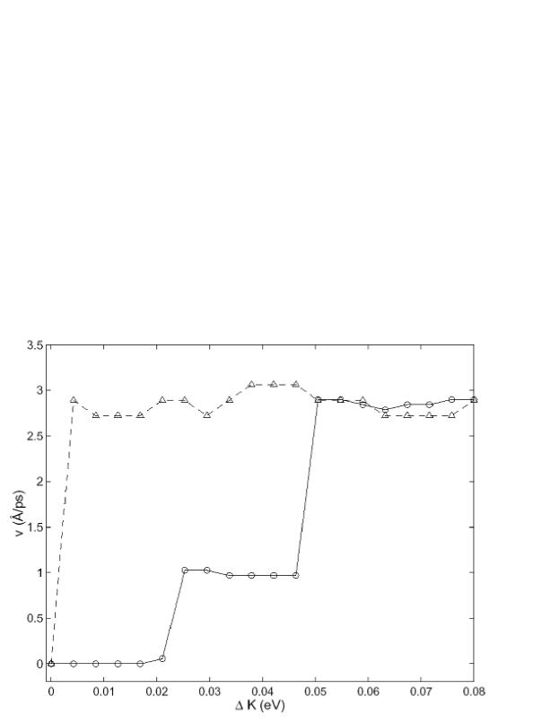
Figure 2: Velocity of the polaron as a function of the energy amount $\Delta K$ corresponding to the mixed regime when the polaron is activated by means of angular perturbations ($\alpha=0.01$). Circles and solid lines represent the disordered case with $\Delta E=0.05$ and triangles and dashed line the ordered case.

3.3 DNA chains with a base-pair inhomogeneity

The studies of polarons in homogeneous chains are only applicable to synthetic DNA made out of a single type of base pair. In real DNA, the two different base pairs, A-T and G-C, combine in different ways constituting the genetic code. Thus, as a first step in this direction, we consider a homogeneous DNA-chain except for a single base pair of a different type. Systems of this type are easily synthesized and the numerical and theoretical results could be compared with the experimental ones. The outcome would help to determine the actual DNA parameters and, therefore, the type of polarons that can be expected. There are two different systems: a) a hard–inhomogeneity, that is, an A-T DNA chain with a C-G inhomogeneity; b) a soft inhomogeneity, i.e., a C-G DNA chain, with an A-T inhomogeneity.

We activate the motion of a stationary polaron, using the discrete gradient method, at a site about a hundred sites far away form the location of the inhomogeneity. Different types of moving polarons can be obtained : radial, twist and mixed ones with different energies, and we observe whether the polarons are reflected, refracted or trapped.

• Soft–inhomogeneity

  In this case, radial polarons moving along a chain of C-G base pairs are trapped by the soft A-T base pair as shown in Fig. 3. Trapping is caused by resonances between the polaron and the stationary state centered at the inhomogeneity.

  

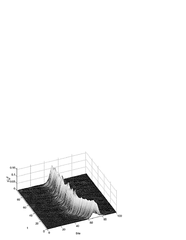
  Figure 3: Soft inhomogeneity and radial polarons. Trapping phenomenon due to the interaction between a moving radial polaron in a C-G chain with an A-T base pair

  However, when the polarons are activated by twist modes, the moving polarons are always transmitted. The inhomogeneity acts as a potential well, as shown in Fig. 4. Note that the polaron adopts briefly the shape of the ground state while passing through the inhomogeneity.

  

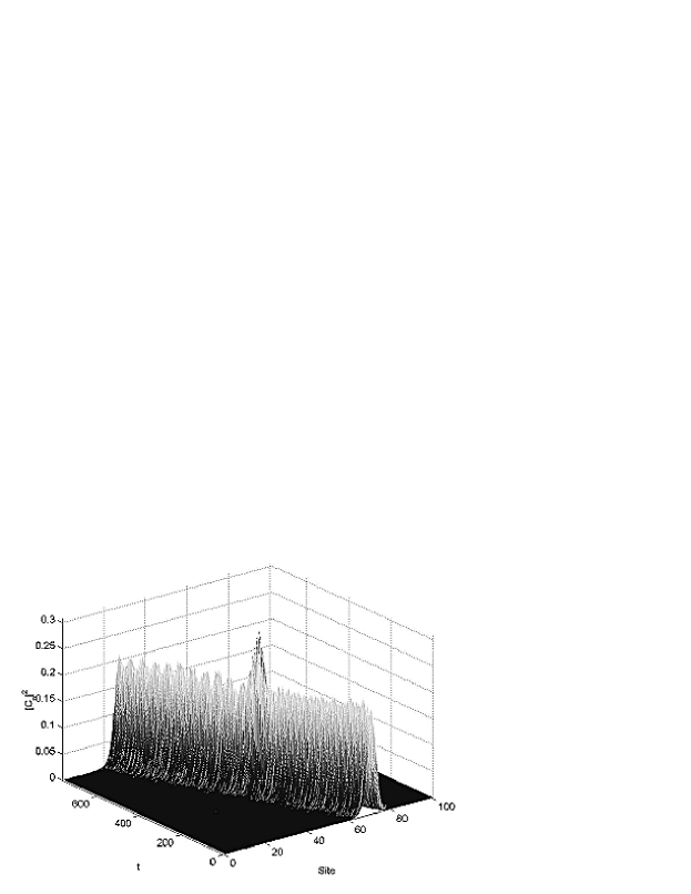
  Figure 4: Soft inhomogeneity and twist polarons. Transmission phenomenon due to the interaction between a moving polaron in a C-G chain with an A-T base pair

• Hard–inhomogeneity

  In this case a radial polaron moving along a chain of A-T base pairs interacts with the C-G inhomogeneity and is always reflected, as is shown in Fig. 5. This phenomenon is due to the impossibility of resonances, because the profiles of the radial components of the polaron and the stationary one located at the inhomogeneity are different.

  

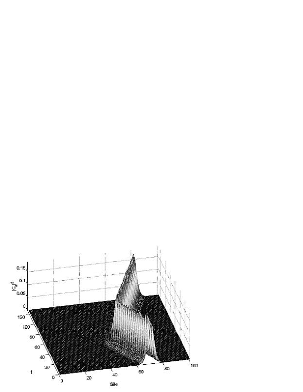
  Figure 5: Hard inhomogeneity and radial polarons. Reflection phenomenon due to the interaction between a moving polaron in an A-T chain with a C-G base pair

  If the moving polaron is of the twist type, it is always transmitted as shown in Fig. 6. In this case the behavior is similar to the movement of a particle through a potential barrier, i.e, its velocity first decreases and then increases until its entering value. Note that again the polaron adopts briefly the shape of the ground state while passing through the inhomogeneity.

  

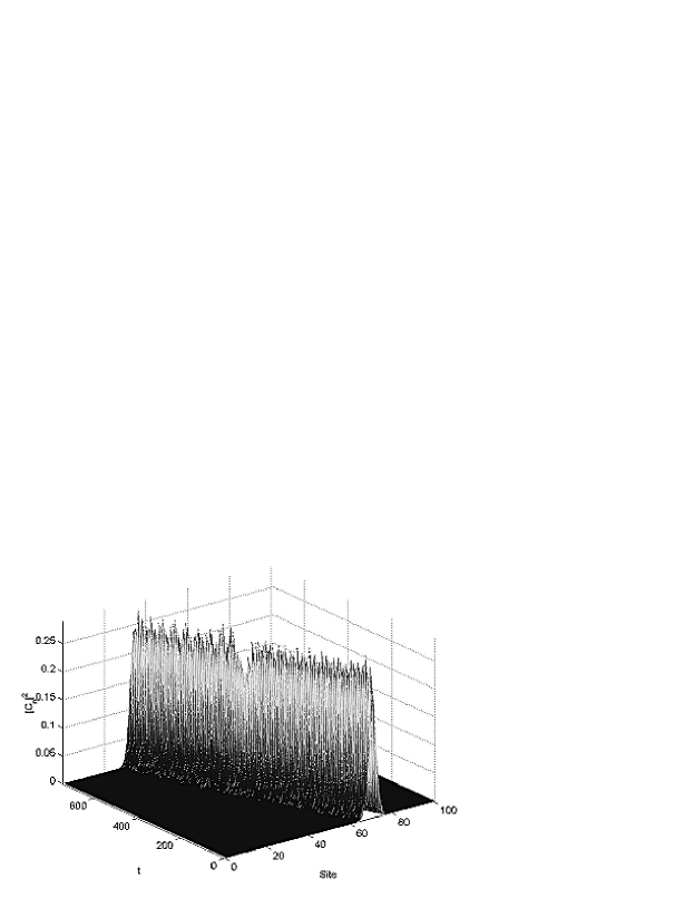
  Figure 6: Hard inhomogeneity and twist polarons. Transmission phenomenon due to the interaction between a moving polaron in an A-T chain with a C-G base pair

In the mixed regime, the phenomena correspond exactly to the type of polaron activated.

Finally, we have performed all the previous simulations introducing a small parametric disorder, in all cases the results are qualitatively similar. These can be summarized in the following table:

	Radial mov.	Twist mov.	Mixed regime.	Mixed regime.
	regime	regime	Radial pert.	Angular pert.
A-T chain	Reflection	Trans.	Reflection	Trans.
C-G chain	Trapping	Trans.	Trapping	Trans.

The results are clear, the only possible candidate for charge transport mediated by polarons in an inhomogeneous chain are the twist modes. Accurate experiments are needed to find out good values of the parameters and for determining which kind of regime is possible in DNA and, therefore, if polarons may have a role in charge transport.

Some preliminary numerical tests with a more realistic model where the ionization energy of a C-G base pair is lower than the A-T base pair by an amount of the order of 0.5 eV, show a trapping phenomenon, similar as the observed experimentally [34], where charge moves in an A-T chain by means of twist modes and reach a C-G base pair. In all other cases we have always observed a reflection phenomenon. This problem will be the object of further research.

4 Conclusions

We have considered a fully nonlinear, three–dimensional, semi–classical, tight–binding model for charge transport in DNA made out of identical base pairs except for a single one of different type, which we call a base pair inhomogeneity. There are two types of this inhomogeneity, soft, composed of G-G base pairs with and A-T inhomogeneity and hard, with the complementary composition.

In a previous work [19], it has been described that in this system there exist two types of polarons, twist polarons and radial polarons, for which the electronic variables are coupled essentially to the radial or angular modes. The existence of these polarons depends both on the system parameters and on the form the movement of the polaron is activated. The properties of the two types of moving polarons are different. In general, the twist polarons are more robust with respect to parametric disorder, the polaron has lower velocity, and the activation energy is higher than in the radial movability regime.

In an inhomogeneous chain with a single different base pair as a local inhomogeneity, we have observed that moving polarons activated by angular perturbations are always transmitted by the inhomogeneity. If the polarons are activated by radial perturbations, we have never observed a transmission of the charge across the inhomogeneity.

Some recent experiments on electron transfer in the DNA molecule [34] show that electrons can migrate over long distances between a triplet C-G base pairs and a C-G base pair separated by a number n of A-T base pairs. Moreover, the triplet C-G base pairs acts as a sink for holes in the chain. In our model, decreasing slightly the ionization energy of the C-G base pair, as in real DNA occurs, we are able to reproduce the experimental results. Some more detailed numerical simulations are currently underway and will be published in due time. Also, these experimental techniques could be of application to contrast experimentally our results.

In our model, we have considered a DNA chain in the vacuum. We have focused in the polaronic character of the charge carrier and its interaction with the chain. If the influence of the medium is not too strong, it is expected that the results would be similar as the ones obtained in the vacuum. In fact, they are in agreement with some experimental observations on DNA in aqueous solutions [34]. The inclusion of thermal effects will be the subject of further studies, although in similar systems it has been shown that the main characteristics of the charge transport do not change very much when the temperature is considered [35].

Appendix A Stationary polaron-like states

In this section we expose the procedure followed for obtaining linearly stable, stationary localized states of our model given by Eqs. (6-8). These solutions have been used in the previous section in order to generate mobile polarons. Since the adiabaticity parameter $\tau$ is small enough, the fastest variables are the $\{c_{n}\}$, with a characteristic frequency (the linear frequency of the uncoupled system) of order $1/\tau\sim 19$, followed by the $\{r_{n}\}$ with frequency unity, and the $\{\phi_{n}\}$ with $\Omega_{\phi}\sim 0.11$. We can suppose initially that $r_{n}$ and $\phi_{n}$ are constant,i.e., we use the Born–Oppenheimer approximation. For this purpose, we use a modification of the numerical method outlined in Refs. [28, 36]. We substitute in Eq. (6) $c_{n}=\Phi_{n}\exp(-\mathrm{i}\,E\,t/\tau)$, with time–independent $\Phi_{n}$’s, and we obtain a nonlinear difference system $E\Phi=\widehat{A}\Phi$, with $\Phi=(\Phi_{1},...,\Phi_{N})$, from which a map $\Phi^{\prime}=\widehat{A}\Phi/\|\widehat{A}\Phi\|$ is constructed, $\|.\|$ being the quadratic norm.

Thus, using Eqs. (6-8), the stationary solutions must be attractors of the map:

$$r^{\prime}_{n} = -\frac{k}{b_{n}}\,|c_{n}|^{2}\$$ (10)

$$-\,\frac{\alpha}{b_{n}}\,\left[\frac{\partial d_{n,n-1}}{\partial r_{n}}(c_{n}^{*}c_{n-1}+c_{n}c_{n-1}^{*})+\frac{\partial d_{n+1,n}}{\partial r_{n}}(c_{n+1}^{*}c_{n}+c_{n+1}c_{n}^{*})\right],$$

$$\phi^{\prime}_{n} = \frac{1}{2}(\phi_{n+1}+\phi_{n-1})\,$$ (11)

$$-\,\frac{\alpha V}{2\Omega^{2}}\,\left[\frac{\partial d_{n,n-1}}{\partial\phi_{n}}(c_{n}^{*}c_{n-1}+c_{n}c_{n-1}^{*})+\frac{\partial d_{n+1,n}}{\partial\phi_{n}}(c_{n+1}^{*}c_{n}+c_{n+1}c_{n}^{*})\right],$$

$$c^{\prime}_{n} = \frac{[(E_{n}\,+k\,r^{\prime}_{n})\,c_{n}-(1-\alpha\,d^{\prime}_{n+1,n})\,c_{n+1}-(1-\alpha\,d^{\prime}_{n\,n-1})\,c_{n-1}]}{\|\{(E_{n}\,+k\,r^{\prime}_{n})\,c_{n}-(1-\alpha\,d^{\prime}_{n+1,n})\,c_{n+1}-(1-\alpha\,d^{\prime}_{n\,n-1})\,c_{n-1}\}\|},$$ (12)

where $d^{\prime}=d(r^{\prime},\phi^{\prime})$. The starting point is a completely localized state given by $c_{n}=\delta_{n,0}$, $r_{n}=0$ and $\phi_{n}=0$, $\forall n$. Then the map is applied until convergence is achieved. In this way both stationary solutions and their energy $E$ can be obtained.

Firstly, we have analyzed the homogeneous and ordered case , i.e., $E_{n}^{0}=E_{0}$, that arises in synthetic DNA (the constant $E_{0}$ can be set to zero by means of a gauge transformation). As shown in Fig. 7, in a typical ground state the charge is fairly localized at few sites, and the amplitudes decay monotonically and exponentially with growing distance from the central site. The associated patterns of the static radial and relative angular displacements are similar

Figure 7: Profiles of the ground state in the homogeneous and ordered chain. (a) Wave function amplitudes $|c_{n}|^{2}$. (b) Static radial displacements $r_{n}$. (c) Static twists elongations $\theta_{nn-1}$

We can introduce a certain degree of parametric disorder in the on–site electronic energy $E_{n}^{0}$ by means of a random potential $E_{n}^{0}\in[-\Delta E,\Delta E]$, with mean value zero and different interval sizes $\Delta E$. In this case, the localized excitation patterns do not change qualitatively, as shown in Fig. 8. However, as the translational invariance is broken by the disorder, the localized excitation pattern is not symmetric with respect to a lattice site, which is different to the ordered case. Also, the localization is enhanced with the disorder, due to Anderson localization [37].

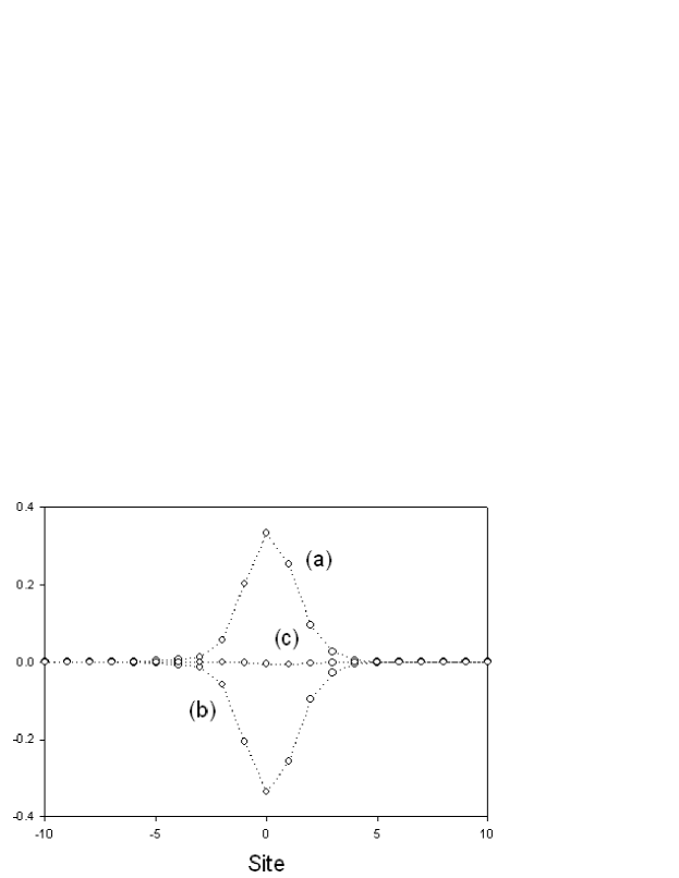
Figure 8: Profiles of the ground state in the homogeneous and disordered chain. (a) Wave function amplitudes $|C_{n}|^{2}$. (b) Static radial displacements $r_{n}$. (c) Static twists elongations $\theta_{nn-1}$

We consider now a chain with a local inhomogeneity due to the existence of a single base pair which is different to the other ones (without disorder). Our results show that the ground state centered in a site far from this local inhomogeneity is qualitatively similar to the obtained in the homogeneous chain case. Nevertheless, differences appear if we consider the stationary state centered in the inhomogeneity. In a C-G chain, with an A-T base pair as the local inhomogeneity, the shape of the ground state is qualitatively similar to the obtained in the homogeneous case, as shown in Fig. 9. In an A-T chain, with a C-G base pair as the local inhomogeneity, the static radial displacements are different, as shown in Fig. 10. As we have seen in the previous section, this fact is determinant in relation with the transmission, reflection or trapping of a moving polaron by the inhomogeneity.

Figure 9: Profiles of the ground state in a C-G chain centered in the inhomogeneity, an A-T base pair. (a) Wave function amplitudes $|C_{n}|^{2}$. (b) Static radial displacements $r_{n}$. (c) Static twists elongations $\theta_{n\,n-1}$

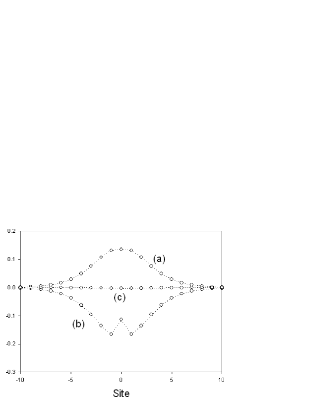
Figure 10: Profiles of the ground state in an A-T chain centered in the inhomogeneity, a C-G base pair.(a) Wave function amplitudes $|C_{n}|^{2}$. (b) Static radial displacements $r_{n}$. (c) Static twists elongations $\theta_{n\,n-1}$

References

- [1] S.M. Gasper and G.B. Schuster. J. Am. Chem. Soc. 119:12762, 1997.
- [2] S. Boiteux, L. Gellon and N. Guibourt. Free Radical Biology and Medicine. 32:1244, 2002.
- [3] C.J. Burrows and J,G. Muller. Chem. Rev. 98:1109, 1998.
- [4] K.A. Friedman and A. Heller. J. Phys. Chem. B. 105:11859, 2001.
- [5] M.E. Núñez, G. Holmquist and J. Barton. Biochem. 40:12465, 2001.
- [6] M.E. Núñez et al. Biochem. 39:6190, 2000.
- [7] E.M. Boon Electrochemical sensors based on DNA–mediated charge transport Chemistry. PhD thesis, 1998.
- [8] C. Mao et al Nature. 407:605, 2000.
- [9] C. Wan et al. Proc. Natl. Acad. Sci. USA. 96:6014, 1999.
- [10] C. Wan et al. Proc. Natl. Acad. Sci. USA. 97:14052, 2000.
- [11] M Ratner. Nature, 397(6719):480, 1999.
- [12] HW Fink and C Schönenberger. Nature, 398(6726):407, 1999.
- [13] P Tran, B Alavi and G Gruner. Phys. Rev. Lett., 85:1564, 2000.
- [14] E Braun, Y Eichen, U Sivan and G Ben-Yoseph. Nature, 391(6669):775, 1998.
- [15] D Porath, A Bezryadin, S de Vries and C Dekker. Nature, 403(6770):635, 2000.
- [16] D Hennig, JFR Archilla, and J Agarwal. Physica D, 180:256, 2003.
- [17] JFR Archilla, D Hennig, and J Agarwal. In L Vázquez, MP Zorzano, and RS Mackay, editors. Localization and Energy Transfer in Nonlinear Systems. World Scientific, 2003. Pages 153–160.
- [18] V. Muto. Nanobiology 1:325, 1992.
- [19] F Palmero, JFR Archilla, D Hennig, and FR Romero. Nonlinear charge transport mediated by twist modes. 2003. Submitted to J. Phys. A, nlin.PS/0301036.
- [20] W Zhang, AO Govorov and SE Ulloa Polarons with a twist. Phys. Rev. B, 66:060303, 2002.
- [21] RN Barnett, CL Cleveland, A Joy, U Landman, and GB Schuster. Science 294:567, 2001
- [22] M Barbi. Localized Solutions in a Model of DNA Helicoidal Structure. PhD thesis, Universitát degli Studi di Firenze, 1998.
- [23] M Barbi, S Cocco and M Peyrard. Phys. Lett. A, 253(5–6):358, 1999.
- [24] M Barbi, S Cocco, M Peyrard and S Ruffo. Jou. Biol. Phys., 24:97, 1999.
- [25] S Cocco and R Monasson. J. Chem. Phys., 112(22):10017, 2000.
- [26] M Salerno Phys. Rev. A,44:5292, 1991.
- [27] G. Brunaud et al. Phys. Chem. Chem. Phys. 4:6072, 2002.
- [28] G Kalosakas, S Aubry and GP Tsironis. Phys. Rev. B, 58(6):3094, 1998.
- [29] L Stryer. Biochemistry. Freeman, New York, 1995.
- [30] H. Sugiyama and I. Saito. J. Am. Chem. Soc. 118:7063, 1996. A.A. Voityuk et al. J. Chem Phys. 114:5614, 2001; H. Zhang et al. J. Chem. Phys. 117:4578, 2002.
- [31] G. Cuniberti et al, Phys. Rev. B. 65:241314, 2002; Y.A. Berlin , A.L. Burin and M.A. Ratner, Superlattices Microstruct. 28:241, 2000.
- [32] D Chen, S Aubry and GP Tsironis. Phys. Rev. Lett., 112(23):4776, 1996.
- [33] M Ibañes, JM Sancho and GP Tsironis. Phys. Rev. E, 65:041902, 2002.
- [34] B Giese, J Amaudrut, K K öhler, M Spormann, and S Wessely Nature, 412:318, 2001
- [35] D. Hennig, J.F.R. Archilla, J. Dorignac and E Starikov Phys. Rev. B. Submitted, 2003.
- [36] NK Voulgarakis and GP Tsironis. Phys. Rev. B, 63:14302, 2001.
- [37] PW Anderson. Phys. Rev., 109:1492, 1958.
- [38] M Peyrard and AR Bishop. Phys. Rev. Lett., 62(23):2755, 1989.
- [39] TD Holstein. Ann. Phys. NY, 8:325, 1959.