Synchronized clusters in coupled map networks: Self-organized and driven phase synchronization

Abstract

We study the synchronization of coupled maps on a variety of networks including regular one and two dimensional networks, scale free networks, small world networks, tree networks, and random networks. The dynamics is governed by a local nonlinear map for each node of the network and interactions connecting different nodes via the links of the network. For small coupling strengths nodes show turbulent behavior but form phase synchronized clusters as coupling increases. We identify two different ways of cluster formation, self-organized clusters which have mostly intra-cluster couplings and driven clusters which have mostly inter-cluster couplings. The synchronized clusters may be of dominant self-organized type, dominant driven type or mixed type depending on the type of network and the parameters of the dynamics. We also observe ideal clusters of both self-organized and driven type. There are some nodes of the floating type that show intermittent behaviour between getting attached to some clusters and evolving independently. The residence times of a floating node in a synchronized cluster show an exponential distribution. We define different states of the coupled dynamics by considering the number and type of synchronized clusters. For the local dynamics governed by the logistic map we study the phase diagram in the plane of the coupling constant ($\epsilon$) and the logistic map parameter ($\mu$). For large coupling strengths and nonlinear coupling we find that the scale free networks and the Caley tree networks lead to better cluster formation than the other types of networks with the same average connectivity. For most of our study we use the number of connections of the order of the number of nodes which allows us to distinguish between the two mechanisms of cluster formation. As the number of connections increases the number of nodes forming clusters and the size of the clusters in general increase.

I Introduction

Several complex systems have underlying structures that are described by networks or graphs and the study of such networks is emerging as one of the fastest growing subject in the physics world Strogatz ; rev-Barabasi . One significant discovery in the field of complex networks is the observation that a number of naturally occurring large and complex networks come under some universal classes and they can be simulated with simple mathematical models, viz small-world networks Watts , scale-free networks scalefree etc. These models are based on simple physical considerations and have attracted a lot of attention from physics community as they give simple algorithms to generate graphs which resemble several actual networks found in many diverse systems such as the nervous systems koch , social groups social , world wide web www , metabolic networks metabolic , food webs food and citation networks citation .

Several networks in the real world consist of dynamical elements interacting with each other. These networks have a large number of degrees of freedom. In order to understand the behaviour of these systems we study the synchronization and cluster formation of these dynamical elements evolving on different networks and connected via the links of the networks.

Synchronization and cluster formation lead to rich spatio-temporal patterns when opposing tendencies compete; the nonlinear dynamics of the maps which in the chaotic regime tends to separate the orbits of different elements, and the couplings that tend to synchronize them. There are several studies on coupled maps/oscillators on regular lattices as well as globally coupled networks. Coupled map lattices with nearest neighbor or short range interactions show interesting spatio-temporal patterns, and intermittent behavior LCM1 ; LCM2 . Globally coupled maps (GCM) where each node is connected with all other nodes, show interesting synchronized behavior GCM1 . Formation of clusters or coherent behaviour and then loss of coherence are described analytically as well as numerically at different places with different points of views GCM2 ; GCM3 ; GCM4 ; GCM5 ; GCM6 ; GCM-phasedia . Chaotic coupled map lattices show beautiful phase ordering of nodes HChate-phase . There are also some studies on coupled maps on different types of networks. Refs. Kaneko-2000 ; H-Chate ; P-Gade shed some light on the collective behavior of coupled maps/oscillators with local and non-local connections. Random networks with large number of connections also show synchronized behavior for large coupling strengths random-net1 ; random-net2 ; random-net3 . There are some studies on synchronization of coupled maps on Cayley tree Tree , small-world networks Small-1 ; Small-2 ; Small-3 and hierarchal organization CHAOS-2002 . Coupled map lattice with sine-circle map gives synchronization plateaus CML-circle . Analytical stability condition for synchronization of coupled maps for different types of linear and non-linear couplings are also discussed in several papers CML-stability1 ; CML-stability2 ; CML-stability3 . Synchronization and partial synchronization of two coupled logistic maps are discussed at length in Ref. bi-partite1 . Apart from this there are other studies that explore different properties of coupled maps REA-gade ; CML-REA ; CML-other1 ; CML-other2 ; CML-other3 .

Coupled maps have been found to be useful in several practical situations. These include fluid dynamics ex-GCM , nonstatistical behavior in optical systems ex-optical , convection ex-Rayleigh ; ex-convection , stock markets ex-stock , ecological systems ex-eco , logic gates ex-CML , solitons ex-soliton and c-elegans ex-celegans .

Here we study the detailed dynamics of coupled maps on different networks and investigate the mechanism of clustering and synchronization properties of such dynamically evolving networks. We explore the evolution of individual nodes with time and study the role of different connections in forming the clusters of synchronized nodes in such coupled map networks (CMNs).

Most of the earlier studies of synchronized cluster formation have focused on networks with large number of connections ($\sim N^{2}$). In this paper, we consider networks with number of connections of the order of $N$. This small number of connections allows us to study the mechanism of synchronized cluster formation and the role that different connections play in synchronizing different nodes. We identify two phenomena, driven and self-organized phase synchronization sarika-REA1 . The connections or couplings in the self-organized phase synchronized clusters are mostly of the intra-cluster type while those in the driven phasen synchronized clusters are mostly of the inter-cluster type. As the number of connections increases more and more nodes are involved in cluster formation and also the coupling strength region where clusters are formed increases in size. For large number of connections, typically of the order of $N^{2}$ and for large coupling strengths, mostly one phase synchronized cluster spanning all the nodes is observed.

Depending on the number and type of clusters we define different states of synchronized behaviour. For the local dynamics governed by the logistic map, we study the phase diagram in the $\mu-\epsilon$ plane, i.e. the plane defined by the logisting map parameter and the coupling constant.

The paper is organized as follows. In section II, we give the model for our coupled map networks. We also define phase synchronization and synchronized clusters as well as discuss the mechanisms of cluster formation. In section III, we present our numerical results for synchronization in different networks and illustrate the mechanism of cluster formation. This section includes the study of the phase diagram, lyapunov exponent plots, behavior of individual nodes, dependence on number of connections, and behaviour for different types of networks. Some universal features of synchronized cluster formation are discussed in section IV. Section V considers circle map. Section VI concludes the paper.

II Coupled maps and synchronized clusters

II.1 Model of a Coupled Map Network (CMN)

Consider a network of $N$ nodes and $N_{c}$ connections (or couplings) between the nodes. Let each node of the network be assigned a dynamical variable $x^{i},i=1,2,\ldots,N$. The evolution of the dynamical variables can be written as

$$x^{i}_{t+1}=(1-\epsilon)f(x^{i}_{t})+\frac{\epsilon}{k_{i}}\sum_{j=1}^{N}C_{ij}g(x^{j}_{t}),$$ (1)

where $x^{i}_{t}$ is the dynamical variable of the $i$-th node at the $t$-th time step and $\epsilon$ is the coupling strength. The topology of the network is introduced through the adjacency matrix $C$ with elements $C_{ij}$ taking values $1$ or $0$ depending upon whether $i$ and $j$ are connected or not. $C$ is a symmetric matrix with diagonal elements zero. $k_{i}=\sum C_{ij}$ is the degree of node $i$. The factors $(1-\epsilon)$ in the first term and $k_{i}$ in the second term are introduced for normalization. The function $f(x)$ defines the local nonlinear map and the function $g(x)$ defines the nature of coupling between the nodes. Here we present detailed results for the logistic map,

$$f(x)=\mu x(1-x)$$ (2)

governing the local dynamics. We have also considered some other maps for local dynamics. We have studied different types of linear and non-linear coupling functions and here discuss the results in detail for the following two types of coupling functions.

$$g(x) = x$$ (3)

$$g(x) = f(x).$$ (4)

We refer to the first type of coupling function as linear and the later as nonlinear.

II.2 Phase synchronization and synchronized clusters

Synchronization of coupled dynamical systems book-syn ; phy-report ; syn-coup is indicated by the appearance of some relations between the functionals of different dynamical variables due to the interactions. The exact synchronization corresponds to the situation where the dynamical variables for different nodes have identical values. The phase synchronization corresponds the situation where the dynamical variables for different nodes have some definite relation between the phases phase1 ; phase2 ; phase3 ; phase4 . When the number of connections in the network is small ($\sim N$) and when the local dynamics of the nodes (i.e. function $f(x)$) is in the chaotic zone, only few clusters with small number of nodes show exact synchronization. However, clusters with larger number of nodes are obtained when we study phase synchronization. For our study we define the phase synchronization as follows syn .

Let $\nu_{i}$ and $\nu_{j}$ denote the number of times the dynamical variables $x^{i}_{t}$ and $x^{j}_{t}$, $t=t_{0},t_{0}+1,2,\ldots,t_{0}+T-1$, for the nodes $i$ and $j$ show local minima during the time interval $T$ starting from some time $t_{0}$. Here the local minimum of $x^{i}_{t}$ at time $t$ is defined by the conditions $x^{i}_{t}<x^{i}_{t-1}$ and $x^{i}_{t}<x^{i}_{t+1}$. Let $\nu_{ij}$ denote the number of times these local minima match with each other, i.e. occur at the same time. We define the phase distance, $d_{ij}$, between the nodes $i$ and $j$ by the following relation note1 ,

$$d_{ij}=1-\frac{\nu_{ij}}{{\rm max}(\nu_{i},\nu_{j})}.$$ (5)

Clearly, $d_{ij}=d_{ji}$. Also, $d_{ij}=0$ when all minima of variables $x^{i}$ and $x^{j}$ match with each other and $d_{ij}=1$ when none of the minima match. In Appendix A, we show that the above definition of phase distance satisfies metric properties. We say that nodes $i$ and $j$ are phase synchronized if $d_{ij}=0$, and a cluster of nodes is phase synchronized if all the pairs of nodes belonging to that cluster are phase synchronized.

II.3 Mechanism of cluster formation

Now we consider the relation between the synchronized clusters which are formed by the dynamical evolution of nodes and the coupling between the nodes of network which is a static property for a given network represented by the adjacency matrix. Clustering is obviously because of the coupling between the nodes of the network and may be achieved in two different ways sarika-REA1 .
(i) The nodes of a cluster can be synchronized because of intra-cluster couplings. We refer to this as the self-organized synchronization.
(ii) Alternately, the nodes of a cluster can be synchronized because of inter-cluster couplings. Here nodes of one cluster are driven by those of the others. We refer to this as the driven synchronization.
We are able to identify ideal clusters of both the types, as well as clusters of the mixed type where both ways of synchronization contribute to cluster formation. We will discuss several examples to illustrate both types of clusters.

II.4 States of synchronized dynamics

We find that as network evolves, it splits into several phase synchronized clusters. The states of the coupled evolving system on the basis of number of clusters can be classified as in Ref. different-region
(a) Turbulent state (I): All nodes behave chaotically with no cluster formation.
(b) Partially ordered state (III): Nodes form a few clusters with some nodes not attached to any clusters.
(c) Ordered state (IV): Nodes form two or more clusters with no isolated nodes at all. This ordered state can be further divided into 3 substates based on the nature of nodes belonging to a cluster. These partitions are chaotic ordered state, quasi-periodic ordered state, and periodic ordered state.
(d) Coherent state (V): Nodes form a single synchronized cluster.
(e) Variable state (II): Nodes form different states, partially ordered or ordered states depending on initial conditions.

In addition to the above definition of states depending on the number of clusters, we further divide the states having synchronized clusters into subcategories depending on the type of clusters i.e. self-organized (S), driven (D) or mixed type (M).

III Numerical results

Now we present the numerical results of the coupled dynamics of variables associated with nodes on different types of networks. Starting from random initial conditions the dynamics of Eq. (1), after an initial transient, leads to interesting phase synchronized behavior. The adjacency matrix $C$ depends on the type of network and $C_{ij}=1$ if the corresponding nodes in the network are connected and zero otherwise. First we will discuss our numerical results in detail for scale-free network and then we will discuss other networks.

III.1 Coupled maps on scale-free network

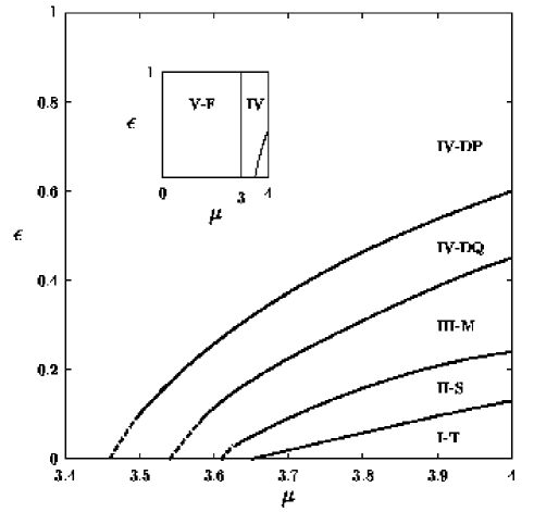
Figure 1: Phase diagram showing different regions in the two parameter space of $\mu$ and $\epsilon$ for scale free network for $f(x)=\mu x(1-x)$ and $g(x)=x$. Different regions based on number of clusters are I. Turbulent region, II. region with varying behaviour, III. Partially ordered region, IV. Ordered region, V. Coherent region. The symbols T, S, M, D, P, Q and F respectively correspond to turbulent behaviour, self-organized synchronization, mixed synchronization, driven synchronization, periodic, quasiperiodic and fixed behaviour. Region boundaries are determined based on the asymptotic behaviour using several initial conditions, number of clusters and isolated nodes, synchronization behaviour and also the behaviour of the largest Lyapunov exponent. The dashed lines indicate uncertainties in determining the boundaries. Calculations are for $N=50,m=1,T=100$. The inset shows the phase diagram for the entire range of parameter $\mu$ i.e. from 0 to 4.

III.1.1 Generation of Network

The scale free network of $N$ nodes is generated by using the model of Barabasi et.al. model . Starting with a small number, $m_{0}$, of nodes, at each time step a new node with $m\leq m_{0}$ connections is added. The probability $\pi(k_{i})$ that a connection starting from this new node is connected to a node $i$ depends on the degree $k_{i}$ of node $i$ (preferential attachment) and is given by

$$\pi(k_{i})=\frac{(k_{i}+1)}{\sum_{j}(k_{j}+1)}.$$

After $\tau$ time steps the model leads to a network with $N=\tau+m_{0}$ nodes and $m\tau$ connections. This model leads to a scale free network, i.e. the probability $P(k)$ that a node has a degree $k$ decays as a power law,

$$P(k)\sim k^{\lambda},$$

where $\lambda$ is a constant and for the type of probability law $\pi(k)$ that we have used $\lambda=3$. Other forms for the probability $\pi(k)$ are possible which give different values of $\lambda$. However, the results reported here do not depend on the exact form of $\pi(k)$ except that it should lead to a scale-free network.

Figure 2: Largest Lyapunov exponent, $\lambda$, is plotted as a function of $\epsilon$ for scale free network and $f(x)=4x(1-x)$ and $g(x)=x$. Different regions are labeled as in Fig. 1.

III.1.2 Linear coupling

Phase diagram: First we start with the linear coupling, $g(x)=x$. Fig. 1 shows the phase diagram in the two parameter space defined by $\mu$ and $\epsilon$ for the scale-free network with $m=m_{0}=1,N=50,T=100$. For $\mu<3$, we get a stable coherent region (region V-F) with all nodes having the fixed point value. To understand the remaining phase diagram, consider the line $\mu=4$. Fig. 2 shows the largest Lyapunov exponent $\lambda$ as a function of the coupling strength $\epsilon$ for $\mu=4$. We can identify four different regions as $\epsilon$ increases from 0 to 1; namely the turbulent region, the variable region (variable behaviour depending on $\epsilon$ and initial conditions), the partially ordered region and the ordered region as shown by regions I to IV in Figs. (1) and (2). The symbols T, S, M, DQ, DP and F correspond to turbulent, self-organized, mixed, driven quasiperiodic, driven periodic and fixed point behaviour. For small values of $\epsilon$, we observe the turbulent behavior with all nodes evolving chaotically and there is no phase synchronization (region I-T). There is a critical value of coupling strength $\epsilon_{c}$ beyond which synchronized clusters can be observed. This is a general property of all CMNs and the exact value of $\epsilon_{c}$ depends on the type of network, the type of coupling function and the parameter $\mu$.

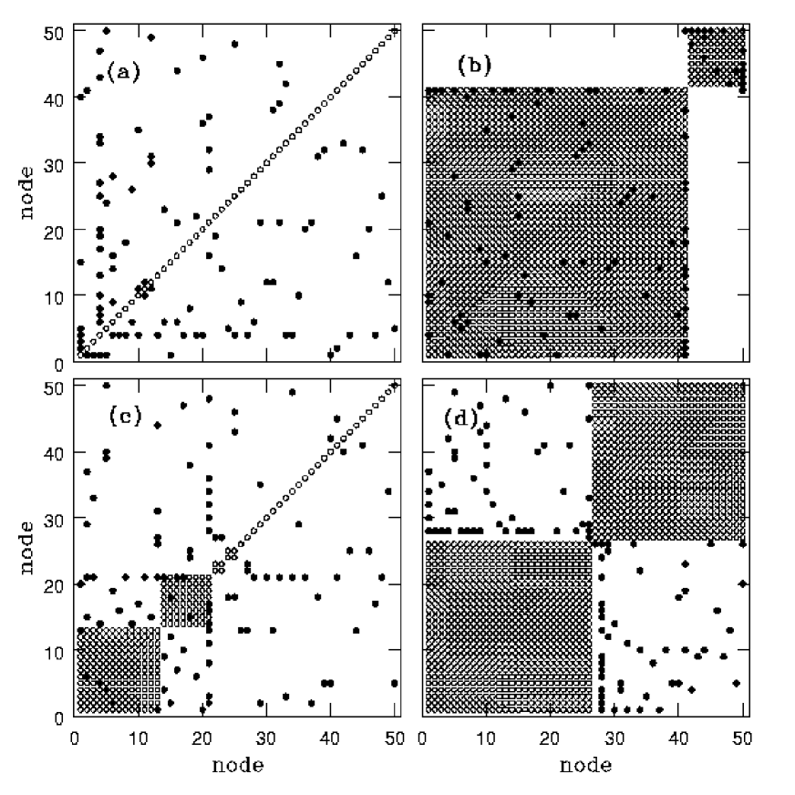
Figure 3: The figure shows several examples illustrating the self-organized and driven phase synchronization. The examples are chosen to demonstrate two different ways of obtaining synchronized clusters and the variety of clusters that are formed. All the figures show node verses node diagram for $N=N_{c}=50$. After an initial transient (about 2000 iterates) pha$N=N_{c}=50$. Afte r an initial transient (about 2000 iterates) phase synchronized clusters are studied for $T=100$. The logistic map parameter $\mu=4$ and coupstudied for $T=100$. The logistic map parameter $\mu=4$ and coupling function $g(x)=x$. The solid circles show that the two corresponding nodes are coupled and the open circles show that the corresponding nodes are phase synchronized. In each case the node numbers are reorganized so that nodes belonging to the same cluster are numbered consecutively and the clusters get displayed in decreasing sizes. (a) Figure shows turbulent phase for $\epsilon=0.10$. (b) An ideal self-organized phase synchronization for $\epsilon=0.16$. (c) Mixed behavior for $\epsilon=0.32$. (d) A ideal driven phase synchronization for $\epsilon=0.90$. The scale free networks were generated with $N_{0}=1$ and $m=1$.

As $\epsilon$ increases beyond $\epsilon_{c}$ we get into a variable region (region II-S) which shows a variety of phase synchronized behavior, namely ordered chaotic, ordered quasiperiodic, ordered periodic and partially orderedbehaviour depending on the initial conditions. The next region (region III-M) shows partially ordered chaotic behavior. Here, the number of clusters as well as the number of nodes in the clusters depend on the initial conditions and also they change with time. There are several isolated nodes not belonging to any cluster. Many of these nodes are of the floating type which keep on switching intermittently between an independent evolution and a phase synchronized evolution attached to some cluster. Last two regions (IV-DQ and IV-DP) are ordered quasiperiodic and ordered periodic regions showing driven synchronization. In these regions, the network always splits into two clusters. The two clusters are perfectly anti-phase synchronized with each other, i.e. when the nodes belonging to one cluster show minima those belonging to the other cluster show maxima.

We now investigate the nature of phase ordering in different regions of the phase diagram. Fig. 3 shows node-node plots of the synchronized clusters with any two nodes belonging to the same cluster shown as open circles and the couplings between the nodes ($C_{ij}=1$) shown as solid circles. For small coupling strength, i.e. region I-T, nodes show turbulent behaviour and no cluster is formed (Fig. 3(a)). In region II-S the dominant behaviour is of self-organized type. Fig. 3(b) shows an ideal self-organized synchronization with two clusters observed in the middle of region II-S. Here, we observe that all the couplings except one are of intra-cluster type. Exactly opposite behavior is observed for the regions IV-DQ and IV-DP. Fig. 3(d) shows an ideal driven synchronization obtained in the middle of region IV-DP. Here, we find that all the couplings are of inter-cluster type with no intra-cluster couplings. This is clearly the phenomena of driven synchronization where the nodes of one cluster are driven into a phase synchronized state due to the couplings with the nodes of the other cluster. The phenomena of driven synchronization in this region is a very robust one in the sense that it is obtained for almost all initial conditions, the transient time is very small, the nodes belonging to the two clusters are uniquely determined and we get a stable solution. In region III-M we get clusters of mixed type (Fig. 3(c)), here the inter-cluster connections and the intra-cluster connections are almost equal in numbers.

Mechanism of cluster formation: We observe that for small values of $\epsilon$ the self organized behavior dominates while for large $\epsilon$ driven behavior dominates. As the coupling parameter $\epsilon$ increases from zero and we enter the region II-S, we observe phase synchronized clusters of the self organized type. Region III-M acts as a crossover region from the self-organized to the driven behavior. Here, the clusters are of the mixed type. The number of inter-cluster couplings is approximately same as the number of intra-cluster couplings. In this region there is a competition between the self-organized and driven behavior. This appears to be the reason for the formation of several clusters and floating nodes as well as the sensitivity of these to the initial conditions. As $\epsilon$ increases, we get into region IV-DQ where the driven synchronization dominates and most of the connections between the nodes are of the inter-cluster type with few intra-cluster connections. This driven synchronization is further stabilized in region IV-DP with two perfectly anti-phase synchronized driven clusters.

Quantitative measure for self-organized and driven behaviour: To get a clear picture of self-organized and driven behaviour we define two quantities $f_{\rm intra}$ and $f_{\rm inter}$ as measures for the intra-cluster couplings and the inter-cluster couplings as follows:

$$f_{\rm intra} = \frac{N_{\rm intra}}{N_{c}}$$ (6)

$$f_{\rm inter} = \frac{N_{\rm inter}}{N_{c}}$$ (7)

where $N_{\rm intra}$ and $N_{\rm inter}$ are the numbers of intra- and inter-cluster couplings respectively. In $N_{\rm inter}$, couplings between two isolated nodes are not included.

Fig. 4 shows the plot of $f_{\rm intra}$ and $f_{\rm inter}$ as a function of the coupling strength $\epsilon$. The figure clearly shows that for small coupling strength (region I-T) both $f_{\rm intra}$ and $f_{\rm inter}$ are zero indicating that there is no cluster formation at all, this is the turbulent region. As the coupling strength increases ($\epsilon$ greater than some critical value $\epsilon_{c}$) we get $f_{\rm intra}\sim 1$ at $\epsilon\sim 0.2$ (region II-S). It shows that there are only intra-cluster couplings leading to self-organized clusters. As coupling strength increases further $f_{\rm intra}$ decreases and $f_{\rm inter}$ increases i.e. there is a crossover from self-organized to driven behavior (regions III-M). As coupling strength enters regions IV-DQ and IV-DP, we find that $f_{\rm inter}$ is large which shows that in this region most of the connections are of the inter-cluster type. In region IV-DP we get $f_{\rm inter}$ almost one corresponding to an ideal driven synchronized behaviour.

Figure 4: The fraction of intra-cluster and inter-cluster couplings, $f_{inter}$ (solid circles) and $f_{intra}$ (open circle) are shown as a function of the coupling strength $\epsilon$ for the scale-free networks with $f(x)=4x(1-x)$ and $g(x)=x$. The figure is obtained by averaging over 20 realizations of the network and 50 random initial conditions for each realization.

Figure 5: Figures show time evolution of nodes belonging to different clusters. This figure is plotted for scale-free network with 50 nodes coupled with $g(x)=x$. (a) A few nodes belonging to two phase synchronized clusters are shown. Nodes denoted by circles belong to one cluster and nodes denoted by squares to another cluster. Here $\epsilon=0.15$. (b) Time series of three nodes which are not phase synchronized with each other arethree nodes which are not phase synchronized with each other are shown with three different symbols. Here, $\epsilon=0.35$.

Behaviour of individual nodes forming clusters: Figs. 5 (a) and (b) show plot of time evolution of some typical nodes. Fig. 5(a) is for nodes in self-organized region ($\epsilon=0.15$), where nodes belonging to the same cluster are marked with the same symbols. It is clearly seen that nodes with the same symbols i.e. belonging to the same cluster are phase synchronized and those belonging to different clusters are completely anti-phase synchronized, i.e. when the nodes in one cluster are showing minima, the nodes in other cluster are showing maxima. (This behaviour is observed for driven behaviour where two clusters are formed, i.e. nodes belonging to different clusters are anti-phase synchronized with each other.) Fig. 5(b) plots the time evolution of three nodes in the partially ordered region ($\epsilon=0.35$). We see that these nodes are not phase synchronized with each other.

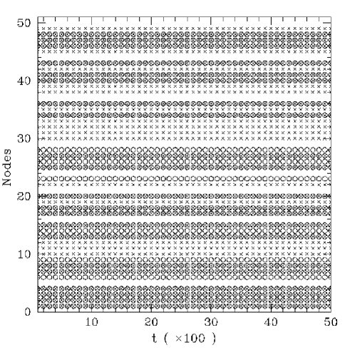
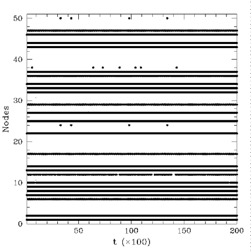
(a) (b)

Figure 6: Figure shows the time evolution of nodes in a cluster for scale-free network. (a) shows two stationary clusters of self-organized type for $\epsilon=0.19$ and $g(x)=x$. The two clusters are for the same $\epsilon$ value but for two different initial conditions. The nodes belonging to the two clusters are denoted by open circles and crosses. Note that some nodes are common to both the clusters while some are different .nodes are common to both the clusters while some are different . This illustrates the nonuniqueness of nodes belonging self-organized clusters depending on the initial conditions. (b) shows a cluster with some permanent nodes and some floating nodes. Here $\epsilon=0.4$ and $g(x)=x$. Node number 12, 24, 38 and 50 are o$\epsilon=0.4$ and $g(x)=x$. Node number 12, 24, 38 and 50 are of floating type. They spend some time intermittently in a synchronized evolution with the given cluster and the remaining time in either a synchronized evolution with other clusters or in an independent evolution as an isolated node.

Now we explore different regions further to understand time evolution of individual nodes attached to some specific cluster. Fig. 6 plots all the nodes belonging to a cluster as a function of time, symbols indicate the time for which a given node belongs to a cluster. First we consider region II-S. Fig. 6(a) shows a set of nodes (crosses) belonging to a cluster in the mixed region for $\epsilon=0.19$ and another set of nodes (open circle) belonging to another cluster for the same $\epsilon$ but obtained with different initial conditions. For this $\epsilon$ value all the nodes form self-organized clusters with no isolated nodes and this cluster formation is stable. It is seen from Fig. 6(a) that all the nodes are permanent members of the cluster. Also comparing the members of two clusters which are obtained from different initial conditions we see that there are some common nodes while some are different. The reason is that these are self-organized clusters and this organization is not unique (see subsection 3.A.4). On the other hand, driven synchronization (region IV-DP) leads to a unique cluster formation and does not depend on the initial conditions.

Next we look at $\epsilon=0.4$ (region III-M) where we get several clusters with some isolated nodes. In Fig. 6(b), nodes belonging to a cluster are plotted as a function of time. We observe that there are some nodes which are attached to this cluster, intermittently leave the cluster, evolve independently or get attached with some other cluster and after some time again come back to the same cluster. These nodes are of the floating type which keep on switching intermittently between an independent evolution and a phase synchronized evolution with some cluster. For example, node number 12 in Fig. (tseries-clus)(b), which forms phase synchronized cluster with other nodes, in between leaves the cluster and evolve independently for some time. Time it spends with the cluster is about 90%. On the other hand node number 24 evolves independently for almost 90% of the time and evolves in phase synchronization with the cluster for the rest of the time.

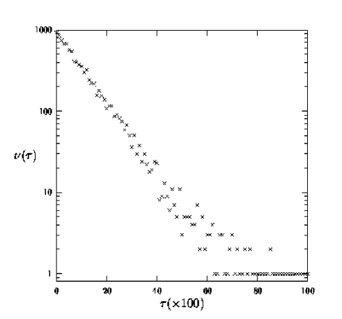
Figure 7: The figure plots the frequency of residence time $f(\tau)$ of a floating node in a cluster as a function of the residence time $\tau$. The data is for node no 12 in Fig. 6(b). A good straight line fit on log-linear plot shows exponential dependence.

Let $\tau$ denote the residence time of a floating node in a cluster (i.e. the continuous time interval that the node is in a cluster). Fig. 7 plots the frequency of residence time $f(\tau)$ of a floating node as a function of the residence time $\tau$. A good straight line fit on log-linear plot shows exponential dependence, $f(\tau)\sim\exp(-\tau/\tau_{r})$ where $\tau_{r}$ is the typical residence time for a given node.

III.1.3 Nonlinear coupling

Now we discuss the results for the nonlinear coupling of the type $g(x)=f(x)$. Phase space diagram in the $\mu-\epsilon$ plane is plotted in Fig. 8. Here we do not get clear and distinct regions as we get for $g(x)=x$ form of coupling. Again the phase diagram is divided into different regions I to V, based on the number of clusters as given in the beginning of this section. For $\mu<3.5$, we get coherent behaviour (regions V-P and VI-F). To describe the remaining phase diagram first consider $\mu=4$ line. Figure 9 shows the largest Lyapunov exponent as a function of the coupling strength $\epsilon$ for $\mu=4$. For small coupling strengths no cluster is formed and we get the turbulent region (I-T). As the coupling strength increases we get into the variable region (II-D). In this region we get partially ordered and ordered chaotic phase depending on the initial conditions. In a small portion in the middle of region II-D, all nodes form two ideal driven clusters. These two clusters are perfectly anti-phase synchronized with each other. Interestingly the dynamics still remains chaotic. In region III-T, we get almost turbulent behaviour with very few nodes forming synchronized clusters. Regions III-M and III-D are partially ordered chaotic regions. In these regions some nodes form clusters and several nodes are isolated or of the floating type.

Figure 8: Phase diagram showing turbulent, phase synchronized and coherent regions in the two parameter space of $\mu$ and $\epsilon$ for scale free network for $f(x)=\mu x(1-x)$ and $g(x)=f(x)$. The determination of region boundaries and their classification and symbols are as explained in Fig. 1. Calculations are for $N=50,m=1,T=100$. The inset shows the phase diagram for the entire range of parameter $\mu$ i.e. from 0 to 4.

Figure 9: Largest Lyapunov exponent, $\lambda$, is plotted as a function of $\epsilon$ for scale-free network and $f(x)=4x(1-x)$ and $g(x)=f(x)$. Different regions are labeled as in Fig. 8.

We now investigate the nature of phase ordering in different regions of the phase diagram. Figs. 10 are node-node plots showing different clusters and couplings (as in Fig. 3) for different $\epsilon$ values belonging to different regions. In Fig. 10(a) (region II-D) we observe that all the couplings are of inter-cluster type with no intra-cluster coupling. This is the phenomenon of driven synchronization. There are two clusters which are perfectly anti-phase synchronized. Fig. 10(b) is plotted for $\epsilon$ in region III-M and it shows clusters of different types. The fifth cluster has only inter-cluster couplings (driven type) while the remaining clusters have dominant intra-cluster couplings (self-organized type). There are several isolated nodes also. Fig. 10(c) shows clusters where the driven behaviour dominates. It is interesting to note that for scale-free network and for this type of nonlinear coupling largest Lyapunov exponent is always positive (Fig. 9) i.e. the whole system remains chaotic but we get phase-synchronized behavior.

Fig. 11 shows the plot of $f_{\rm intra}$ and $f_{\rm inter}$ as a function of the coupling strength $\epsilon$ for $\mu=4$. For small coupling strength both quantities are zero showing the turbulent region, and as the coupling strength increases clusters are formed. $f_{\rm inter}$ is one at $\epsilon\approx 0.13$ which shows that here all the nodes are forming clusters and the clusters are of the driven type having only inter-cluster connections. As the coupling strength increases further, $f_{\rm inter}$ and $f_{\rm intra}$ become almost zero (region III-T) and subsequently start increasing slowly (region III-M) but we see that $f_{\rm inter}$ is always greater than $f_{\rm intra}$ leading to dominant driven phase synchronized clusters. For $\epsilon>0.7$, $f_{\rm intra}$ starts decreasing and for $\epsilon>0.8$, the driven behaviour becomes more prominent (region III-D and Fig. 10(c)). For the regions III-M and III-D, we get phase synchronized clusters but the size of clusters as well as the number of nodes forming clusters both are small.

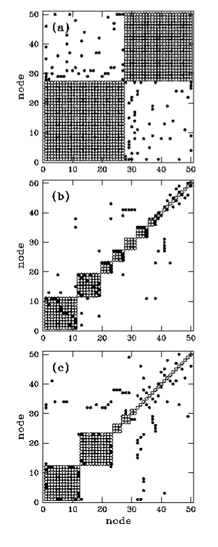
Figure 10: The figure shows several examples illustrating the phase synchronization for scale-free network with coupling form $g(x)=f(x)$ using node verses node diagram for $N=N_{c}=50$. After an initial transient (about 2000 iterates) phase synchronized clusters are studied for $T=100$. The logistic map parameter $\mu=4$. The solid circles show that the two corresponding nodes are coupled and the open circles show that the corresponding nodes are phase synchronized. In each case the node numbers are reorganized so that nodes belonging to the same cluster are numbered consecutively and the clusters get displayed in decreasing sizes. (a) Figure show an ideal driven phase synchronization for $\epsilon=0.13$. (b) Mixed behavior for $\epsilon=0.71$. (c) A dominant driven behavior for $\epsilon=0.88$. The scale free networks were generated with $N_{0}=1$ and $m=1$.

III.1.4 Network geometry and Cluster formation

Geometrically, the organization of the scale-free network into connections of both self-organized and driven types is always possible for $m=1$. For $m=1$, our growth algorithm generates a tree type structure. A tree can be broken into different clusters in two distinct ways.
(a) A tree can be broken into two or more disjoint clusters with only intra-cluster couplings by breaking one or more connections. Clearly, this splitting is not unique. This behaviour is observed in region II-S of the phase-diagram in Fig. 1 and can be seen by comparing Fig. 3(b) of this paper (two ideal self-organized cluster of sizes 41 and 9) and Fig. 1(a) of Ref. sarika-REA1 (two ideal self-organized cluster of sizes 36 and 14) which are plotted for the same scale free network and $g(x)=x$ but for different $\epsilon$ values.
(b) A tree can also be divided into two clusters by putting connected nodes into different clusters. This division is unique and leads to two clusters with only inter-cluster couplings. This behaviour is observed in region IV-DP of the phase-diagram in Fig. 1 and can be seen by comparing Fig. 3(d) of this paper and Fig. 1(b) of Ref. sarika-REA1 which are again plotted for the same scale free network but for diferrent $\epsilon$ values.

Figure 11: The fraction of intra-cluster and inter-cluster couplings, $f_{inter}$ (solid circles) and $f_{intra}$ (open circle) are shown as a function of the coupling strength $\epsilon$ for the scale-free networks with $g(x)=f(x)$. The figure is obtained by averaging over 20 realizations of the network and 50 random initial conditions for each realization.

For $m>1$ and $g(x)=x$ the dynamics of Eq. (1) leads to a similar phase diagram as in Fig. (1) with region II-S dominated by self-organized synchronization and regions IV-DQ and IV-DP dominated by driven synchronization. Though perfect inter- and intra-cluster couplings between the nodes as displayed in Figs. (3b) and  (3d) are no longer observed, clustering in the region II-S is such that most of the couplings are of the intra-cluster type while for the regions IV-DQ and IV-DP they are of the inter-cluster type. As $m$ increases the regions I and II are mostly unaffected, but the region IV shrinks and the region III grows in size. Fig. 12 shows different types of clusters in node-node diagram for different coupling strength. Fig. 12(a) is plotted for $m=3$ in the variable region ($\epsilon=0.19$) with nodes forming two clusters. It is clear that synchronization of nodes is mainly because of intra-cluster connections but there are a few inter-cluster connections also. Fig. 12(b) is plotted for the ordered periodic region at coupling strength $\epsilon=0.78$, here the clusters are mainly of the driven type but they have intra-cluster connections also. In Figures 12(a) and (b) the average degree of a node is 6, and breaking the network into clusters with only inter-cluster or intra-cluster couplings is not possible. As the average degree of a node increases further self-organized behaviour starts dominating and for most of the $\epsilon$ values nodes behave in phase-synchronized manner forming one big cluster.

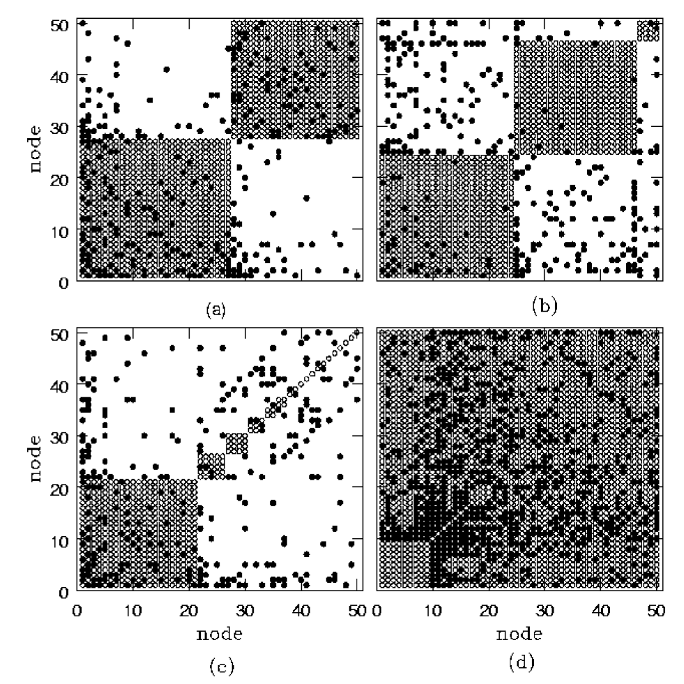
Figure 12: Figure illustrates the cluster formation for the scale-free network as node vs node plot for $N=50$ as in Fig. 3 but with larger number of connections. (a) and (b) are plotted for $g(x)=x$ and $m=3$ and respectively for $\epsilon=0.19$ and $\epsilon=0.78$. (c) and (d) are plotted for $g(x)=f(x)$, $\epsilon=0.90$ and respectively for $m=3$ and $m=10$.

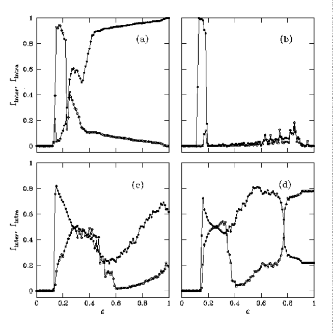
Figure 13: The fraction of intra-cluster and inter-cluster couplings, $f_{inter}$ (solid circles) and $f_{intra}$ (open circles) are shown as a function of the coupling strength $\epsilon$. Figures (a) and (b) are for the one-d coupled maps with nearest neighbor coupling ($m=1$) and for $g(x)=x$ and $g(x)=f(x)$ respectively. Figures (c) and (d) are for $g(x)=f(x)$ and respectively $m=5$ and $m=10$. The figures are for $N=50$ and are obtained by averaging over 50 random initial conditions.

For $m>1$ and $g(x)=f(x)$ we get similar kind of behaviour as for $m=1$ with dominant driven clusters for most of the coupling strength region, but we do not get any ideal driven clusters. Fig. 12(c) is plotted for coupling strength $\epsilon=0.9$ and $m=3$. As $m$ increases the region I showing turbulent behaviour remains unaffected, but the mixed region II grows in size while the region III shrinks. As $m$ increases more and more nodes participate in cluster formation. The driven behaviour decreases in strength with increasing $m$ and self-organized behaviour increases in strength. For $m=10$, all nodes form one cluster for larger $\epsilon$ values which is obviously of the self-organized type (Fig. 12(d)).

We have also studied the effect of size of the network on the synchronized cluster formation. The phenomena of self-organized and driven behavior persists for the largest size network that we have studied ($N=1000$). The region II showing self-organized or driven behavior is mostly unaffected while the ordered regions showing driven behavior for large coupling strengths show a small shrinking in size.

III.2 Coupled maps on one dimensional network

For one dimensional CMN, each node is connected with $m$ nearest neighbors (degree per node is $2m$). First we consider $m=1$, i.e each map is connected with just next neighbors on both sides. Fig .13(a) and (b) show $f_{\rm intra}$ and $f_{\rm inter}$ verses $\epsilon$ for $g(x)=x$ and $g(x)=f(x)$ respectively and $\mu=4$, $N=50$. For $g(x)=x$, after an initial turbulent region ($\epsilon>\epsilon_{c}$), nodes form self-organized clusters (region II-S in Fig. 1) and as the coupling strength increases we observe a crossover to driven clusters. The behaviour of clusters as well as Lyapunov exponent graphs are similar to the scale-free network with the coupling form $f(x)=x$. Note that the nearest neighbor CMN with $m=1$ is a tree and can be geometrically organized into both self-organized and driven type of clusters.

Figure 14: Largest Lyapunov exponent, $\lambda$, is plotted as a function of $\epsilon$ for 1-d nearest neighbor coupled network for $f(x)=4x(1-x)$ and $g(x)=f(x)$. Different regions are labeled as for scale-free network (see Fig. 8 and Fig. 9.)

For $g(x)=f(x)$ coupling and $m=1$, there is cluster formation for only small coupling strength region (corresponding to region II-D of Fig. 8) as seen from Fig 13(b). Fig. 14 shows largest Lyapunov exponent as a function of $\epsilon$ for $g(x)=f(x)$ and $\mu=4.0$. In region II-D the largest Lyapunov exponent is positive or negative, depending on the initial conditions and $\epsilon$ values and for the rest of the coupling strength region Lyapunov exponent is positive. In region II-D synchronized clusters of driven type are seen. For larger coupling strengths where the system remains in chaotic zone, clusters are rarely formed and when formed are small in size.

Fig. 15 shows node-node plot showing synchronized clusters. Fig. 15(a) shows one self-organized cluster in region II-S (see Fig. 1) for $g(x)=x$. In this region we also get two self-organized clusters depending on the initial values and $\epsilon$. Fig. 15(b) shows two clusters of mixed type as well as several isolated nodes for $\epsilon$ in region III-M for $g(x)=x$. Figures 15(c) and 15(d) show driven clusters for $g(x)=f(x)$ for $\epsilon$ values in regions II-D of Fig. 14.

We now consider the case $m>1$. For $g(x)=x$ we observe self-organized clusters with some inter-cluster connections for the coupling strength region II-S and as the coupling strength increases there is a crossover to driven clusters. As the coupling strength increases further for $\epsilon>0.7$ instead of forming driven clusters (as is observed for $m=1$) nodes form one synchronized cluster. As $m$ increases $f_{intra}$ increases and for $\epsilon>\epsilon_{c}$ we observe dominance of self-organized behaviour. For $m=5$, and for coupling strength $\epsilon>\epsilon_{c}(\approx 0.13)$, all nodes form one or two clusters. For one cluster $f_{intra}=1$ and for two clusters intra-cluster and inter-cluster couplings are almost equally distributed. For very large value of coupling strength ($\epsilon>0.7$) we get clusters of dominant self-organized type. As the number of connections increases and typically becomes of the order $N^{2}$ that is a globally coupled state, we get one cluster of self-organized type.

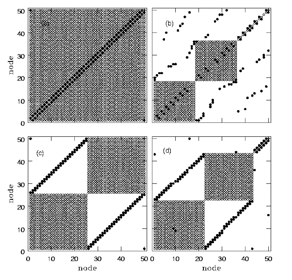
Figure 15: The figure illustrates the cluster formation for one-d nearest neighbor network using node-node plot as in Fig. 3. (a) and (b) are for $g(x)=x$ and $\epsilon=0.16$, and $\epsilon=0.30$ respectively. (c) and (d) are for $g(x)=f(x)$ and $\epsilon=0.13$ and $\epsilon=0.15$ respectively.

Figure 16: Figure (a) shows the fraction of nodes forming clusters as a function of the fraction of couplings $N_{c}/N_{m}$ where $N_{m}=N(N-1)/2$. The figures are plotted for 1-d coupled maps with $g(x)=f(x)$ and for $\epsilon=0.49$ (closed circles) and $\epsilon=0.7$ (open circles). The results are for $N=50$ and are obtained by averaging over 100 random initial conditions. Figure (b) shows the fraction of nodes in the largest cluster as a function of $N_{c}/N_{m}$ for $\epsilon=0.49$ (closed circles) and $\epsilon=0.7$ (open circles). Other parameters are same as above.

For $g(x)=f(x)$ and $m>1$, we find that as the number of connections increases for small coupling strength (region II-D) we get two dominant driven phase synchronized clusters. For large coupling strength the number of nodes forming clusters and the sizes of clusters both increase with the increase in number of connections in the network. This behaviour is seen in Figs. 13(c) and (d) which show $f_{\rm intra}$ and $f_{\rm inter}$ verses $\epsilon$ for $g(x)=f(x)$, $\mu=4$ and respectively for $m=5$ and $m=10$. Fig. 16(a) shows the fraction of nodes forming clusters as a function of the number of connections $N_{c}$ normalized with respect to the maximum number of connections $N_{m}=N(N-1)/2$ for two values of $\epsilon$. The overall increase in the number of nodes forming clusters is clearly seen. Fig. 16(b) shows the fraction of nodes in the largest cluster as a function $N_{c}$ for two values of $\epsilon$. The overall growth in the size of the clusters with $N_{c}$ is evident.

Figure 17: Frction of intra-cluster and inter-cluster couplings, $f_{inter}$ (solid line) and $f_{intra}$ (dashed line) are shown as a function of the coupling strength $\epsilon$. Figures (a) and (b) are for the small world network for $g(x)=x$ and $g(x)=f(x)$ respectively and $N=50$. Figures (c) and (d) are for the Caley tree with $g(x)=x$ and $g(x)=f(x)$ respectively and $N=47$. The figures are obtained by averaging over 50 random initial conditions. Small world networks are generated with $m=1$ and $p=0.06$ [3]. Caley trees are generated with coordination number three [27].

Cluster formation with large number of connections (of the order of $N^{2}$) and its dependence on coupling strength is discussed in Refs. CML-critical1 ; CML-critical2 . It is reported that for these networks it is the coupling strength which affects the synchronized clusters and not the number of connections. We find that when the number of connections is of the order of $N$ there are significant deviations from this reported behaviour. We find that the size of the clusters and number of nodes forming clusters increases as the number of connections increase as discussed above. This behaviour approaches the reported behaviour as the number of connections increases and becomes of the order of $N^{2}$.

III.3 Coupled maps on Small world network

Small world networks are constructed using the following algorithm by Watts and Strogatz Watts . Starting with a one-dimension ring lattice of $N$ nodes in which every node is connected to its nearest $k$ neighbors ($k/2=m$ on either side), we randomly rewire each connection of the lattice with probability $p$ such that self-loops and multiple connections are excluded. Thus, $p=0$ gives a regular network and $p=1$ gives a random network. Here we present results for $N=50$ and $m=1$. Figs. 17(a) and 17(b) plot $f_{\rm intra}$ and $f_{\rm inter}$ for $g(x)=x$ and $g(x)=f(x)$ respectively as a function of $\epsilon$ for $\mu=4$. We find that for $g(x)=x$, the behaviour is very similar to that for the scale free networks and one-d lattice. We get self-organized clusters for $\epsilon>\epsilon_{c}$ and there is a crossover to driven behavior as epsilon increases (Fig. 17(a) ). But for $g(x)=f(x)$, nodes form clusters only for region II-D of coupling strength and there is almost no cluster formation for larger values of $\epsilon$ ( Fig. 17(b) ). This behaviour changes as $k$ increases and we observe some clusters for large $\epsilon$ values also. Figure 18(a) shows node-node plot of clusters for $\epsilon=0.45$, $m=1$ and $g(x)=x$ showing dominant driven clusters.

III.4 Coupled maps on Caley Tree

We generate a Caley tree using the algorithm given in Ref. Tree . Starting with three branches at the first level, we split each branch into two at subsequent levels. For $g(x)=x$, the behaviour is similar to all other networks with the same number of connections (Fig. 17(c)). Figure 18(b) shows node-node plot of two ideal driven phase synchronized clusters for $\epsilon=0.92$, $\bar{k}=2$, $N=47$ and $g(x)=x$. For $g(x)=f(x)$ all nodes form driven clusters for region II-D, and for larger coupling strengths about 40% of nodes form clusters of driven types (Fig. 17)(d)).

III.5 Coupled maps on higher dimensional lattices

Coupled maps on higher dimensional lattices also form synchronized clusters. First we give the result for two-d square lattices. Figs. 19(a) and 19(b) plot $f_{\rm intra}$ and $f_{\rm inter}$ for $g(x)=x$ and $g(x)=f(x)$ respectively as a function of $\epsilon$ for $\mu=4$. For $g(x)=x$ the cluster formation is similar to other networks described earlier except for very large $\epsilon$ close to one where we get a single self-organized cluster. For $g(x)=f(x)$ cluster formation is similar to that in one-d networks with nearest and next nearest neighbor couplings. In small coupling strength region II-D (see Figure 8), nodes form two clusters of driven type and for large coupling strength also driven clusters are observed with 25-30% nodes showing synchronized behaviour (Figure. 19(b)). Figures 18(c) and (d) show node-node plot of self-organized behaviour for $g(x)=x$ and dominant driven behaviour for $g(x)=f(x)$.

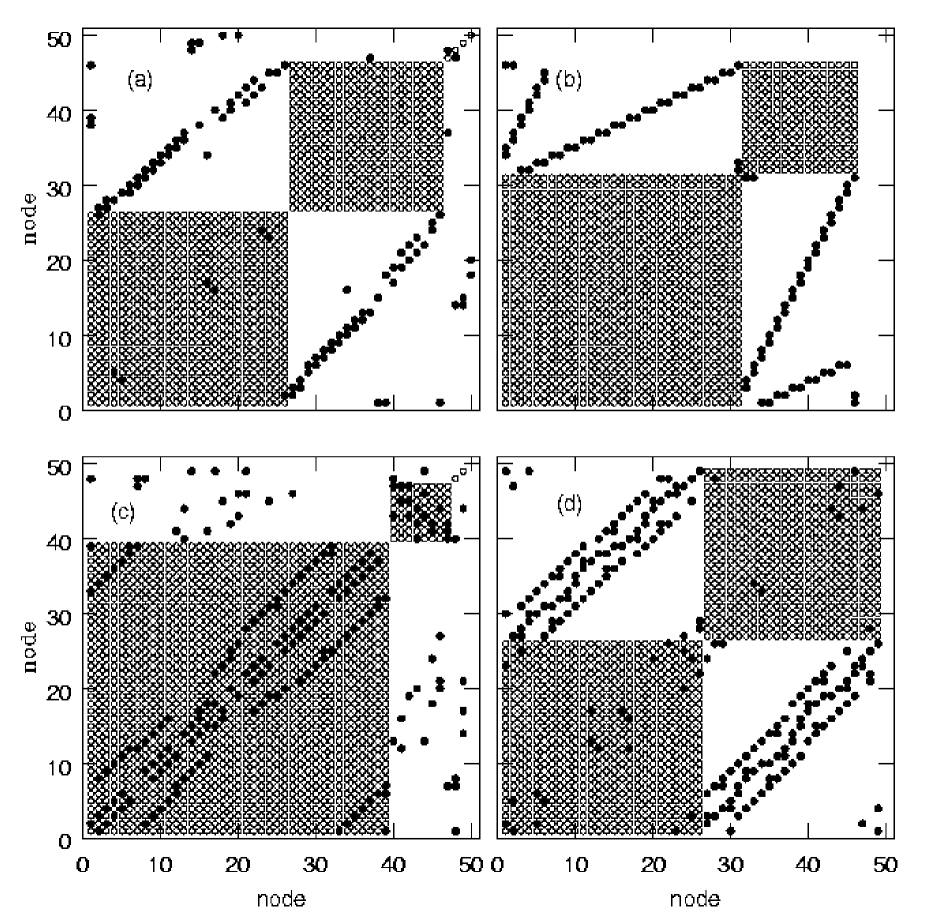
Figure 18: Figure illustrates the cluster formation for different networks as node vs node plot as in Fig 3. (a) is plotted for small world network with $\epsilon=0.45$, $N=50$ and $g(x)=x$. (b) is plotted for Caley tree with $\epsilon=0.92$, $N=47$ and $g(x)=x$. (c) and (d) are plotted for 2-d lattice ($N=49$) with $\epsilon=0.21$, $g(x)=x$ and $\epsilon=0.19,g(x)=f(x)$ respectively.

Coupled maps on three-d cubic lattice (degree per node is six) for $g(x)=x$ show clusters similar to the other networks discussed earlier. For $g(x)=f(x)$, nodes form driven type of clusters at small coupling strength (region II-D) and mainly we observe three clusters. For large coupling strengths also nodes form driven clusters and the nodes participating in cluster formation is now much larger than the two-d case.

III.6 Coupled maps on random network

Random networks are constructed by connecting each pair of nodes with probability $p$. First consider the case where the average degree per node is two. For linear coupling $g(x)=x$ cluster formation is the same as for other networks with same average degree. For $g(x)=f(x)$ driven type clusters are observed in region II-D and no significant cluster formation is observed for larger coupling strengths. This behaviour is similar to one-d network with $k=2$ but different from the corresponding scale free network. For coupled maps on random networks with average degree per node equal to four and $g(x)=f(x)$, clusters with dominant driven behaviour are observed for all $\epsilon>\epsilon_{c}$.

III.7 Examples of self-organized and driven behavior

There are several examples of self-organized and driven behaviour in naturally occurring systems. An important example in physics that includes both self-organized and driven behavior, is the nearest neighbor Ising model treated using Kawasaki dynamics. As the strength of the Ising interaction between spins changes sign from positive to negative there is a change of phase from a ferromagnetic (self-organized) to an antiferromagnetic (driven) behavior. In the antiferromagnetic state, i.e. driven behavior, the lattice spits into two sub-lattices with only inter-cluster interactions and no intra-cluster interactions.

Several other examples are discussed in Ref. sarika-REA1 .

Figure 19: The fraction of intra-cluster and inter-cluster couplings, $f_{inter}$ (solid line) and $f_{intra}$ (dashed line) are shown as a function of the coupling strength $\epsilon$ for two-d lattice. Figures (a) and (b) are for $g(x)=x$ and $g(x)=f(x)$ respectively. The figures are for $N=49$ and are obtained by averaging over 50 random initial conditions.

IV Universal features

We have discussed the behavior of evolution of coupled dynamical elements on different networks. For small coupling strengths unto a critical value $\epsilon_{c}$ nodes show turbulent behaviour and for $\epsilon>\epsilon_{c}$ they form interesting phase-synchronized clusters. The critical value $\epsilon_{c}$ depends on the type of network, the type of coupling function and parameter $\mu$. We find that clusters are formed because of intra-cluster connections and/or inter-cluster connections depending on the network, the type of coupling and the coupling strength.

The linear coupling of type $g(x)=x$ shows both types of clusters (self-organized and driven) and show a behaviour which is universal for all the networks that we have studied. For networks, with number of connections of the order of $N$, initially for a small range of coupling strength (region II-S in Figure 1) nodes form self-organized clusters and as coupling strength increases there is a crossover and reorganization of nodes to driven clusters. This behaviour is observed for all the networks that we have studied i.e. scale-free network, random network, small world network, Caley tree network, 1-d nearest neighbor coupled network, 1-d next to next neighbor coupled network, 2-d network. As the number of connections, $N_{c}$, increases, the driven behaviour for large coupling strengths is suppressed and self-organized behaviour starts dominating. As $N_{c}$ increases further a clear identification of the two mechanisms, self-organized and driven, becomes more and more difficult. As $N_{c}$ becomes of the order of $N^{2}$, for very large coupling strengths we observe one spanning cluster of self-organized type.

For coupling function $g(x)=f(x)$ the formation of clusters and nature of clusters both depend on the type of network. Initially for a small range of coupling strength values (region II-D in Fig. 8) nodes form driven clusters for all networks but as coupling strength increases cluster formation and size of clusters both depend on the type of network. For networks with average connectivity per node equal to two, we find that for large coupling strengths number of nodes forming clusters and size of clusters both are small. For large coupling strengths where largest Lyapunov exponent is positive, less than 50% nodes form clusters for scale-free network and Caley tree. For other types of networks cluster formation is not significant. As the total number of connections increases from $N_{c}\sim N$ to $N_{c}\sim N^{2}$, the number of nodes forming clusters as well as the size of clusters increase. Again as in the case of $g(x)=x$ for very large coupling strengths one large spanning cluster is observed.

It is interesting to note that nodes can form two or more stationary clusters even though coupled dynamics is in the chaotic regime. Here, a stationary cluster means that constituents of the cluster are unique and once nodes form a stationary cluster they belong to that cluster forever, that is the structure of the cluster does not depend on time. For $\mu=4$, we get stationary clusters when the nodes form two clusters, but they are not stationary when they form three or more clusters. Note that three or more stationary clusters can be formed for $\mu<4$.

For $\mu=4$ if the largest Lyapunov exponent is negative, the variables show periodic behaviour with even period. For $\mu<4$ the periodic behaviour can have both odd and even periods.

We observe ideal behaviour of both the types that is all the nodes forming driven clusters ($f_{inter}=1$) or all the nodes forming self-organized clusters ($f_{inter}=1$). In most cases where ideal behaviour is observed, the largest Lyapunov exponent is negative or zero giving stable clusters. However, in some cases ideal behaviour is also observed in the chaotic region.

V Circle map

We have studied cluster formation by considering circle map as defining the local dynamics, given by

$$f(x)=x+\omega+(k/2\pi)sin(2\pi x),\,\pmod{1}$$

Due to the modulo condition, instead of using the variable $x_{t}$, we use a function of $x_{t}$ such as $\sin(\pi x_{t})$ satisfying periodic boundary conditions to decide the location of maxima and minima which are used to determine the phase synchronization of two nodes (Eq. (5)). With circle map also we observe formation of clusters with the time evolution starting from initial random conditions. Here we discuss the results with the parameters of the circle map in the chaotic region ($\omega=0.44$ and $k=6$). For linear coupling $g(x)=x$ and scale-free networks with $m=1$, for small coupling strength nodes evolve chaotically with no cluster formation. As coupling strength increases nodes form clusters for $0.21<\epsilon<0.25$. In most of this region the nodes form two cluster and these clusters are mainly of the driven type except in the initial part, $\epsilon\approx 0.21$, where self-organized clusters can be observed. As the coupling strength increases nodes behave in a turbulent manner and after $\epsilon>0.60$ nodes form clusters of dominant driven type. Here the number of nodes forming clusters and the sizes of clusters, both are small. For the one dimensional linearly coupled networks, for linear coupling the nodes form phase synchronized clusters for coupling strength region $0.21<\epsilon<0.25$. The clusters are mainly of the driven type except in the initial part, $\epsilon\approx 0.21$, where they are of the self-organized type. For large coupling strength they do not show any cluster formation.

For $g(x)=f(x)$ we found very negligible cluster formation for the entire range of the coupling strength for both scale free and one-d network. However, as $m$ increases the nodes form phase synchronized clusters for $\epsilon$ larger than some critical $\epsilon_{c}$.

For the circle map the normalization factor $(1-\epsilon)$ in the first term of Eq. (1) is not necessary and the following modified model can also be considered.

$$x^{i}_{t+1}=f(x^{i}_{t})+\frac{\epsilon}{k_{i}}\sum_{j=1}^{N}C_{ij}g(x^{j}_{t}),\;\;\pmod{1}.$$ (8)

We now discuss the synchronized cluster formation for the same parameter values as above ($\omega=0.44$ and $k=6$) for this modified model. For linear coupling, clusters are formed only for $0.02<\epsilon<0.17$ with dominant self-organizied behaviour for most of the range except near $\epsilon\approx 0.17$ where the behaviour is of doninant driven type. For the scale free networks ($m=1$) we have ordered states while for the one-d networks we have partially ordered states. For nonlinear coupling, the clusters are formed for $0.0<\epsilon<0.09$. The scale-free networks show mostly mixed type clusters while one-d networks show dominant self-organized clusters. There is no cluster formation for larger coupling strengths for both linear and nonlinear coupling. However, as for the logistic map, synchronized clusters are obseved for large $\epsilon$ as the number of connections inceases.

VI Conclusion and Discussion

We have studied the properties of coupled dynamical elements on different types of networks. We find that in the course of time evolution they show phase synchronized cluster formation. We have mainly studied networks with small number of connections $(N_{c}\sim N)$ because a large number of natural systems fall under this category of small connections. More importantly, with small number of connections, it is easy to identify the relation between the dynamical evolution, the cluster formation and the geometry of networks. We have studied the mechanism of cluster formation as well as behaviour of individual nodes either forming clusters or evolving independently. We use the logistic map for the local dynamics and the two types of couplings. Depending upon the type of coupling, the regions for cluster formation and the behaviour of phase synchronization vary. We have identified two mechanism of cluster formation, self-organized and driven phase synchronization.

By considering the number of inter- and intra-cluster couplings we can identify phase synchronized clusters with dominant self-organized behavior (S), dominant driven behavior (D) and mixed behavior (M) where both mechanisms contribute. We have also observed ideal clusters of both self-organized and driven type. In most cases where ideal behaviour is observed, the largest Lyapunov exponent is negative or zero giving stable clusters with periodic evolution. However, in some cases ideal behaviour is also observed in the chaotic region. In most of the cases when synchronized clusters are formed there are some isolated nodes which do not belong to any cluster. More interestingly there are some floating nodes which show an intermittent behavior between an independent evolution and an evolution synchronized with some cluster. The time spent by a floating node in the synchronized cluster shows an exponential distribution.

By defining different states of the dynamical system using the number and type of clusters, we consider the phase-diagram in the $\mu-\epsilon$ plane for the local dynamics governed by the logistic map. When the local dynamics is in the chaotic region, for small coupling strengths we observe turbulent behaviour. There is a critical value $\epsilon_{c}$ above which phase synchronized clusters are observed. For $g(x)=x$ type of coupling, self-organized clusters are formed when the strength of the coupling is small. As the coupling strength increases there is a crossover from the self-organized to the driven behavior which also involves reorganization of nodes into different clusters. This behaviour is almost independent of the type of networks. For non linear coupling of type $g(x)=f(x)$, for small coupling strength phase synchronized clusters of driven type are formed, but for large coupling strength number of nodes forming cluster as well as size of cluster both are very small and almost negligible for many network. Only for scale-free networks and Caley tree show some cluster formation for large coupling strengths.

As the number of connections increases, most of the clusters become of the mixed type where both the mechanisms contribute. We find that in general, the self-organized behaviour is strengthened and also the number of nodes forming clusters as well as the size of clusters increase. As the number of connections become of the order of $N^{2}$, self-organized behaviour with a single spanning cluster is observed for $\epsilon$ larger than some value.

It is interesting to consider the dynamical origin of the self-organized and driven phase synchronization. A clue can be obtained by considering small networks of two or three nodes and also tailormade large networks such as globally coupled networks and complete bipartite networks. These are considered in Ref. pre2 . These studies reveal that the intra-cluster coupling term between the two varibles $x^{i}$ and $x^{j}$, adds a decay term to the dynamics of the difference variable $x^{d}=x^{i}-x^{j}$ leading to synchronization of these two variables. On the other hand, the inter-cluster coupling term between the two varibles $x^{i}$ and $x^{j}$, cancels out in the dynamics of $x^{d}$ and the two variables now belong to different synchronized clusters.

In this paper we have discussed the numerical results of phase synchronization on CMN and the two mechanisms of cluster formation. In another paper we discuss the stabilty analysis of synchronized clusters in some simple networks that illustrate the two mechanisms of synchronization pre2 .

Appendix A

Here we show that the definition (5) of phase distance $d_{ij}$ between two nodes $i$ and $j$ satisfies metric properties. Let ${\cal N}_{i}$ denote the set of minima of the variable $x^{i}_{t}$ in a time interval $T$. The phase distance satisfies the following metric properties.
(A) $d_{ij}=d_{ji}$.
(B) $d_{ij}=0$ only if ${\cal N}_{i}={\cal N}_{j}$.
(C) Triangle inequality: Consider three nodes $i$, $j$ and $k$. Denoting the number of elements of a set by $|.|$, let,
(1) $a=|{\cal N}_{i}\cap{\cal N}_{j}\cap{\cal N}_{k}$.
(2) $b=|{\cal N}_{i}\cap{\cal N}_{k}|-a$.
(3) $c=|{\cal N}_{j}\cap{\cal N}_{k}|-a$.
(4) $d=|{\cal N}_{i}\cap{\cal N}_{j}|-a$.
(5) $e=|{\cal N}_{i}|-b-d-a$.
(6) $f=|{\cal N}_{j}|-c-d-a$.
(7) $g=|{\cal N}_{k}|-b-c-a$.
We have

$$n_{ik} = a+b$$

$$n_{jk} = a+c$$

$$n_{ij} = a+d$$

$$n_{i} = a+b+d+e$$

$$n_{j} = a+c+d+f$$

$$n_{k} = a+b+c+g$$

Consider the combination

$$d_{ik}+d_{jk}-d_{ij}=1-X$$ (9)

where

$$X=\frac{n_{ik}}{{\rm max}(n_{i},n_{k})}+\frac{n_{jk}}{{\rm max}(n_{j},n_{k})}-\frac{n_{ij}}{{\rm max}(n_{i},n_{j})}$$

The triangle inequality is proved if $X\leq 1$. Consider the following three general cases.

• $n_{i}\leq n_{j}\leq n_{k}$:
  

  $$X = \frac{a+b}{n_{k}}+\frac{a+c}{n_{k}}-\frac{a+d}{n_{j}}$$ (10)

  $$\leq \frac{a+b+c-d}{n_{k}}$$

  $$\leq 1$$

• $n_{i}\leq n_{k}\leq n_{j}$:
  

  $$X = \frac{a+b}{n_{k}}+\frac{a+c}{n_{j}}-\frac{a+d}{n_{j}}$$ (11)

  $$\leq \frac{a+b+c}{n_{k}}$$

  $$\leq 1$$

• $n_{k}\leq n_{i}\leq n_{j}$:
  

  $$X = \frac{a+b}{n_{i}}+\frac{a+c}{n_{j}}-\frac{a+d}{n_{j}}$$ (12)

  $$\leq \frac{a+b+c}{n_{i}}$$

  $$\leq \frac{a+b+c}{n_{k}}$$

  $$\leq 1$$

This proves the triangle inequality.

References

- (1) S. H. Strogatz, Nature, 410, 268 (2001) and references theirin.
- (2) R. Albert and A. L. Barabäsi, Rev. Mod. Phys. 74, 47 (2002) and references theirin.
- (3) D. J. Watts and S. H. Strogatz, Nature (London) 393, 440 (1998).
- (4) A. -L. Barabäsi, R. Albert, Science, 286, 509 (1999).
- (5) C. Koch and G. Laurent, Science 284, 96 (1999).
- (6) S. Wasserman and K. Faust, Social Network Analysis, Cambridge Univ. Press, Cambridge 1994.
- (7) R. Albert, H. Jeong, A. -L. Barabäsi, Nature 401, 130 (1999); R. Albert, H. Jeong, A. -L. Barabäsi, Nature 406, 378 (2000).
- (8) H. Jeong, B. Tomber, R. Albert, Z. N. Oltvai, A. -L. Barabäsi, Nature, 407, 651 (2000).
- (9) Richard J. Williams, Nea D. Martinez, Nature, 404, 180 (2000).
- (10) S. Render, Euro. Phys. J. B. 4, 131 (1998); M. E. J. Newman, Phys. Rev. E 64 016131 (2001).
- (11) K. Kaneko, Prog. Theo. Phys. 72 No. 3, 480 (1984).
- (12) K. Kaneko, Physica D, 34, 1 (1989), and references therein.
- (13) K. Kaneko, Phys. Rev. Lett. 65, 1391 (1990); Physica D, 41, 137 ( 1990 ); Physica D, 124, 322 (1998).
- (14) D. H. Zanette and A. S. Mikhailov, Phys. Rev. E 57, 276 (1998).
- (15) N. J. Balmforth, A. Jacobson and A. Provenzale, CHAOS 9, 738 (1999).
- (16) O. Popovych, Y. Maistenko and E. Mosekilde, Phys. Lett. A, 302, 171 (2002).
- (17) G. I. Menon, S. Sinha, P. Ray, (Europhy. Let.) arXiv:cond-mat/0208243.
- (18) O. Popovych, A. Pikovsky and Y. Maistrenko, Physica D, 168-169, 106 (2002).
- (19) G. Abramson and D. H. Zanette, PRE, 58, 4454 (1998).
- (20) A. Lemaître and H. Chate, Phys. Rev. Lett. 82, 1140 (1999).
- (21) N. B. Ouchi and K Kaneko, Chaos 10, 359 (2000).
- (22) H. Chate and P. Manneville, Europhys. Lett. 17, 291 (1992); Chaos 2 3, 307 (1992).
- (23) P. M. Gade, Phys. Rev. E 54, 64 (1996).
- (24) C. Susanna, Manrubia and A. S. Mikhailov, PRE, 60, 1579 (1999).
- (25) Y Zhang, G. Hu, H. A. Cerderia, S. Chen, T. Barun and Y. Yao, PRE 63, 63 (2001).
- (26) S. Sinha, PRE 66 016209 (2002).
- (27) P. M. Gade and H. A. Cerderia, R. Ramaswamy, PRE 52, 2478 (1995).
- (28) P. M. Gade and C.-K. Hu, Phys. Rev. E 62, 6409 (2000);
- (29) H. Hong, M. Y. Choi and B. J. Kim, Phys. Rev. E 65 026139 (2002); Phys. Rev. E 65 047104 (2002).
- (30) T. Nishikawa, A. E. Motter, Y. C. Lai and F. C. Hoppensteadt, Phys. Rev. Lett. 91, 014101 (2003).
- (31) N. J. Balmforth, A. Provenzale and R. Sassi, CHAOS 12, 719 (2002).
- (32) S. E. de S. Pinto and R. L. Viana, Phys. Rev. E 61 5154 (2000).
- (33) H. Fujisaka and T. Yamada, Prog. Theo. Phys. 69 32 (1983).
- (34) M. Ding and W. Yang, Phys. Rev. E 56, 4009 (1997).
- (35) M. Soins and S. Zhou, Physica D 165, 12 (2002).
- (36) J. Jost and M. P. Joy, Phys. Rev. E 65, 016201 (2002).
- (37) Y. L. Maistrenko, V. L. Maistrenko, O. Popovych and E. Mosekilde, Phys. Rev. E, 60 2817 (1999).
- (38) R. E. Amritkar, P. M. Gade and A. D. Gangal, Phys. Rev. A 44, R3407 (1991).
- (39) R. E. Amritkar, Physica A, 224, 382 (1996).
- (40) E. Olbrich, R. Hegger and H. Kantz, Phys. Rev. Lett. 84 2132 (2000).
- (41) P. Garcïa, A. Parravano, M. G. Cosenza, J. Jimënez and A. Marcano, Phys. Rev. E 65 045201-1 (2002).
- (42) L. Cisneros, J. Jimënez, M. G. Cosenza and A. Parravano, Phys. Rev. E 65 045204-1 (2002).
- (43) H. Aref, Ann. Rev. Fluid Mech. 15, 345 (1983)
- (44) G. Perez, C. Pando-Lambruschini, S. Sinha and H. A. Cerderia, Phys. Rev. A, 45 5469 (1992).
- (45) E. A. Jackson and A. Kodogeorgiou, Phys. Lett. A, 168, 270 (1992).
- (46) T. Yanagita and K. Kaneko, Phys. Lett. A, 175, 415 (1993).
- (47) C. Tsallis, A. M. C. de Souza and E. M. F. Curado, Chaos, Solitons and Fractals, 6, 561 (1995).
- (48) R. J. Hendry, J. M. McGlade and J. Weiner, Ecological Modeling, 84, 81 (1996).
- (49) S. Sinha and W. L. Ditto, Phys. Rev. Lett., 81, 2156 (1998).
- (50) K. Aoki and N. Mugibayashi, Phys. Lett. A, 128, 349 (1998).
- (51) F. A. Bignone, Theor. Comp. Sci., 217 157 (1999).
- (52) S. Jalan, R. E. Amritkar, Phys. Rev. Lett. 90, 014101 (2003).
- (53) A. Pikovsky, M. Rosenblum and J. Kurth, Synchronization : A universal concept in nonlinear dynamics (Cambridge University Press, 2001).
- (54) S. Boccaletti, J. Kurth, G. Osipov, D.L. Valladares and C. S. Zhou, Physics Report, 366 (1-2), (2002), The synchronization of chaotic systems.
- (55) Y. Zhang, G. Hu, H. A. Cerdeira, S. Chen, T. Braun and Y. Yao, Phys. Rev. E 63 026211-1 (2001).
- (56) M. G. Rosenblum, A. S. Pikovsky, and J. Kurth, PRL, 76, 1804 (1996); W. Wang, Z. Liu, Bambi Hu, Phys. rev. Lett. 84, 2610 (2000).
- (57) S. C. Manrubia and A. S. Mikhailov, Europhys. Lett. 53 (4), 451 (2001).
- (58) N. B. Janson, A. G. Balanov, V. S. Anishchenko and P. V. E. McClintock, Phys. Rev. Lett. 86 1749 (2001).
- (59) H. L. Yang, Phys. Rev. Lett. 64 026206-1 (2001).
- (60) F. S. de San Roman, S. Boccaletti, D. Maza and H. Mancini, Phys. Rev. Lett. 81, 3639 (1998).
- (61) In an earlier paper sarika-REA1 we used the definition of phase distance as . However, this earlier definition does not satisfy the triangle inequality, while the definition given in this paper satisfies the same.
- (62) S. C. Manrubia and A. S. Mikhailov, arXiv:cond-mat/9912054 v1 3 Dec 1999.
- (63) A. -L. Barabasi, R. Albert, H. Jeong, Physica A, 281, 69 (2000).
- (64) S. Sinha, D. Biswas, M. Azam and S. V. Lawande, Phys. Rev. A 46 6242 (1992).
- (65) V. Ahlers and A. Pikovsky, Phys. Rev. Lett. 88 254101 (2002).
- (66) S. Jalan, R. E. Amritkar and C. K. Hu, unpublished.