Travel time stability in weakly range-dependent sound channels

Abstract

Travel time stability is investigated in environments consisting of a range-independent background sound-speed profile on which a highly structured range-dependent perturbation is superimposed. The stability of both unconstrained and constrained (eigenray) travel times are considered. Both general theoretical arguments and analytical estimates of time spreads suggest that travel time stability is largely controlled by a property $\omega^{\prime}$ of the background sound speed profile. Here, $2\pi/\omega(I)$ is the range of a ray double loop and $I$ is the ray action variable. Numerical results for both volume scattering by internal waves in deep ocean environments and rough surface scattering in upward refracting environments are shown to confirm the expectation that travel time stability is largely controlled by $\omega^{\prime}$.

2002

205

5

Dated: ]

LABEL:FirstPage1

LABEL:LastPage#1102

identifier

I Introduction

Measurements made during the Slice89 propagation experiment Duda-etal-92 , performed in the eastern North Pacific Ocean, suggested that in that environment the near-axial energy is more strongly scattered than the energy corresponding to the steeper rays. Similar behavior was subsequently observed in measurements made during the AET experiment Worcester-etal-99 ; Colosi-etal-99 , also performed in the eastern North Pacific Ocean. Motivated in large part by these observations, several studies Duda-Bowlin-94 ; Simmen-Flatte-Yu-Wang-97 ; Smirnov-Virovlyansky-Zaslavsky-01 ; Beron-Brown-03 have been carried out to investigate the dependence of ray stability on environmental parameters. All of these studies have focused on ray stability in either physical space (depth, range) or phase space (depth, angle). The present study extends the earlier work by considering the sensitivity of ray travel times to environmental parameters. Our focus on travel times is more closely linked to the Slice89 and AET observations than the earlier sensitivity studies inasmuch as both sets of measurements were made in depth and time at a fixed range.

In this study we consider ray motion in environments consisting of a range-independent background on which a range-dependent perturbation, such as that produced by internal waves in deep ocean environments, is superimposed. We consider the influence of the background sound speed structure on both unconstrained and constrained (eigenray) measures of travel time spreads. Surprisingly, the conclusion of this work is that travel time stability is largely controlled by the same property Beron-Brown-03 of the background sound speed structure that controls ray trajectory stability. Although this work was motivated by the deep ocean measurements mentioned above, the results presented apply to a much larger class of problems. To illustrate this generality we include numerical simulations of ray scattering by a rough surface in upward refracting environments.

The remainder of the paper is organized as follows. In Sec. II the equations on which our analysis is based are presented. These are the coupled ray/travel time equations written in terms of both the usual phase space variables and action–angle variables. In Sec. III two simple expressions for unconstrained travel time spreads in terms of action–angle variables are derived (trivially) and shown to be in good agreement with numerical simulations. In Sec. IV an expression for constrained (eigenray) time spreads is derived, again using action–angle variables, and shown to be in good agreement with numerical simulations. The same result was recently derived using a different argument by Virovlyansky Virovlansky-03 . The combination of the results presented in Secs. III and IV provide strong evidence that, quite generally, travel time spreads are largely controlled by the same property $\omega^{\prime}=\mathrm{d}\omega/\mathrm{d}I$ of the background sound speed structure. Here, $2\pi/\omega(I)$ is the range of a ray double loop and $I$ is the ray action variable. In Sec. V our results are summarized and discussed. Two explanations for why $\omega^{\prime}$ controls travel time spreads are given.

II Background

A Theory

This paper is concerned with the scattering of sound, in the geometric limit, by weak inhomogeneities. Consistent with these assumptions, our analysis is based on the one-way form (cf. e.g. Ref. Brown-etal-03, and references therein) of the ray equations, 

$$\frac{\mathrm{d}p}{\mathrm{d}r}=-\frac{\partial h}{\partial z},\quad\frac{\mathrm{d}z}{\mathrm{d}r}=\frac{\partial h}{\partial p},$$ (1a)

and travel time equation,

$$\frac{\mathrm{d}T}{\mathrm{d}r}=p\frac{\mathrm{d}z}{\mathrm{d}r}-h,$$ (1b)

where

$$h(p,z,r)=-\sqrt{c^{-2}(z,r)-p^{2}}.$$ (2)

Here, $r$, which is the independent variable, denotes range; $z$ is depth; $p$ is vertical ray slowness; $T$ is travel time; and $c(z,r)$ is sound speed. Equations (1) constitute a canonical Hamiltonian system with $h$ the Hamiltonian, $(z,p)$ the generalized coordinate–conjugate momentum pair, and $T$ playing the role of the mechanical action. It follows from Eqs. (1a) and $\mathrm{d}z/\mathrm{d}r=\tan\varphi$, where the ray angle $\varphi$ is measured relative to the horizontal, that $cp=\sin\varphi.$ We shall assume the sound speed to be the sum of a range-independent background component, $C(z)$, plus a (weak) range-dependent perturbation, $\delta c(z,r)$. This allows us to write the Hamiltonian as the sum of a range-independent (integrable) component, $H(p,z)=-\sqrt{C^{-2}(z)-p^{2}}$, plus a range-dependent (nonintegrable) perturbation, $\delta h(p,z,r)\approx-\delta c(z,r)/[C^{3}(z)H(p,z)].$

In the background environment, i.e. when $\delta c=0,$ the ray motion is naturally described using action–angle variables $(I,\vartheta)$. The transformed ray equations maintain their Hamiltonian structure with Hamiltonian $\bar{H}(I)=H(p(I,\vartheta),z(I,\vartheta)),$ namely

$$\frac{\mathrm{d}I}{\mathrm{d}r}=-\frac{\partial\bar{H}}{\partial\vartheta}=0,\quad\frac{\mathrm{d}\vartheta}{\mathrm{d}r}=\frac{\partial\bar{H}}{\partial I}=\omega(I).$$ (3a)

The travel time equation, in turn, reads

$$\frac{\mathrm{d}T}{\mathrm{d}r}=I\omega-\bar{H}+\frac{\mathrm{d}}{\mathrm{d}r}\left(G-I\vartheta\right).$$ (3b)

Here,

$$G(z,I)=\pi I\pm\int_{z_{-}}^{z}\mathrm{d}\xi\,\sqrt{C^{-2}(\xi)-\bar{H}^{2}(I)},$$ (4)

where the $\pm$ sign applies to $\pm p,$ is the (multiply-valued) generating function of the canonical transformation that relates implicitly the new variables $(I,\vartheta)$ to the original variables $(p,z)$ through

$$p=\frac{\partial G}{\partial z},\quad\vartheta=\frac{\partial G}{\partial I}.$$ (5)

The action variable is defined by

$$I=\frac{1}{2\pi}\oint\mathrm{d}z\,p=\frac{1}{\pi}\int_{z_{-}}^{z_{+}}\mathrm{d}z\,\sqrt{C^{-2}(z)-H^{2}},$$ (6)

where the loop integral is taken along an isoline of $H$ and thus $z_{\pm}$ correspond to the ray upper $(+)$ and lower $(-)$ turning depths.

Equations (3a) show that in the background environment each ray trajectory forms a closed loop in $(p,z)$-space, or phase space, on which $I$ is a constant. The line integral in Eq. (6) can also be expressed as an integral over the enclosed area in phase space. It follows from Eq. (6) that $I=0$ for the axial ray and that $I$ increases monotonically as axial ray angle increases. For rays making multiple loops $G$ advances by $2\pi I$ and $\vartheta$ advances by $2\pi$ each time a loop is completed. Following a ray, the difference $G-I\vartheta$ makes small oscillations about zero. The term $\mathrm{d}(G-I\vartheta)/\mathrm{d}r$ gives small endpoint contributions to $T.$ The fractional contributions from this term to $T$ are nonnegligible only at very short range. The contribution from this term to several of the analytical travel time spread estimates presented below is zero. In those cases where this contribution is not identically zero, it is very small.

In range-dependent environments, i.e. with $\delta c\neq 0,$ action–angle variables can be defined using the same relations as in the unperturbed environment Abdullaev-Zaslavsky-91 . This is in fact possible because the range-independent canonical transformation $(p,z)\mapsto(I,\vartheta)$ depends solely on the geometry of phase space, characterized by the symplectic two-form $\mathrm{d}p\wedge\mathrm{d}z,$ which is the same with $\delta c=0$ or $\delta c\neq 0;$ it does not depend on the Hamiltonian itself (cf. e.g. Ref. Arnold-89, ). It is important to realize, however, that in the presence of a range-dependent pertubation $\delta c,$ the action variable $I$ as defined in Eq. (6) is not constant anymore because $H$ is not a first integral of (1). The Hamiltonian in the new variables takes the form $\bar{H}(I)+\delta\bar{h}(I,\vartheta,r)$, where $\bar{H}(I)=H(p(I,\vartheta),z(I,\vartheta))$ and $\delta\bar{h}(I,\vartheta,r)=\delta h(p(I,\vartheta),z(I,\vartheta),r).$ The ray and travel time equations then read

$$\frac{\mathrm{d}I}{\mathrm{d}r}=-\frac{\partial\delta\bar{h}}{\partial\vartheta},\quad\frac{\mathrm{d}\vartheta}{\mathrm{d}r}=\omega+\frac{\partial\delta\bar{h}}{\partial I},$$ (7a)

and

$$\frac{\mathrm{d}T}{\mathrm{d}r}=I\frac{\mathrm{d}\vartheta}{\mathrm{d}r}-\bar{H}-\delta\bar{h}+\frac{\mathrm{d}}{\mathrm{d}r}\left(G-I\vartheta\right).$$ (7b)

In realistic ocean environments Eqs. (7) are difficult to apply because in such environments the dependence of $\delta h$ on $I$ and $\vartheta$ is not known explicitly. Because of this, most of the results presented below assume that the environment is piecewise range-independent. These results follow from piecewise application of Eqs. (3). This procedure eliminates difficulties associated with the lack of availability of an explicit expression for $\delta\bar{h}(I,\vartheta,r).$ The endpoint correction term $\mathrm{d}(G-I\vartheta)/\mathrm{d}r$ in (3b) will be neglected throughout the reminder of this paper.

The reason for introducing action–angle variables is that these variables provide the most succinct description of the underlying ray dynamics. The equations presented in the next three sections that make use of action–angle variables can also be written in terms of the original phase space variables $(p,z),$ but the $(p,z)$ form of the equations are more complicated and obscure the important role, described below, played by $\omega^{\prime}$ in controlling travel time spreads.

B Some qualitative features of scattered ray travel time distributions

Some basic features of ray travel times in deep-ocean environments without and with internal-wave-induced scattering are shown in Fig. 1. Travel time and ray depth are plotted at $r=2$ Mm for rays emitted from an axial source in each of the two sound channels shown in Fig. 2. The nonscattered ray travel times plotted in Fig. 1 correspond to rays with launch angles $\varphi_{0}$ confined to $4^{\circ}$ bands. The scattered ray travel times plotted in Fig. 1 correspond to an ensemble of $200$ rays with a fixed launch angle, each in the same background sound speed structure but with an independent realization of the internal-wave-induced perturbation superimposed. (Independent realizations were generated using the same internal wave field by staggering the initial range at which rays were launched with $\Delta r=5$ km; the vertical derivative of internal-wave-induced sound speed perturbations has a horizontal correlation length shorter than $5$ km Brown-Viechnicki-98 , so this simple procedure ensures statistical independence.) Figure 1 shows two examples of a portion of what is commonly referred to as a timefront, consisting of many smooth branches that meet at cusps.

Figure 1: (a) Ray travel time and depth at $r=2$ Mm in the C0 sound channel (cf. Fig. 2) without (solid curve) and with (dots) internal-wave-induced sound speed perturbations superimposed. The source is on the sound channel axis in both cases. In the absence of internal-wave-induced perturbations $8^{\circ}\leq\varphi_{0}\leq 12^{\circ},$ where $\varphi_{0}$ is ray launch angle. In the presence of internal-wave-induced perturbations $\varphi_{0}=10^{\circ}$ in each of 200 realizations of the internal wave field. (b) Same as (a) except that the C14 sound speed was used with $10^{\circ}\leq\varphi_{0}\leq 14^{\circ}$ without internal-wave-induced perturbations, and $\varphi_{0}=12^{\circ}$ with internal-wave-induced perturbations.

The internal-wave-induced sound speed perturbation used to produce Fig. 1—and all subsequent numerical calculations shown in this paper that include internal-wave-induced sound speed perturbations—was computed using Eq. (19) of Ref. Colosi-Brown-98, . In that expression $y$ and $t$ were set to zero, i.e. a frozen vertical slice of an internal wave field was assumed. The range-averaged buoyancy frequency profile measured during the AET experiment was used. The dimensionless strength parameters $E$ and $\mu$ were taken to be $6.3\times 10^{-5}$ and $17.3,$ respectively. Horizontal wavenumber and vertical mode number cutoffs of $2\pi$ $\mathrm{km}^{-1}$ and $30,$ respectively, were used. The resulting sound speed perturbation field is highly structured and fairly realistically describes a typical deep-ocean midlatitude internal-wave-induced sound speed perturbation.

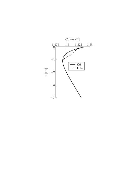
Figure 2: Background sound speed profiles used in the numerical work presented in Figs. 1, 3, 4, 8, 9 and 10.

Figure 1 shows that internal-wave-induced scattering is predominantly along the background timefront. Internal-wave-induced scattering also causes a broadening of individual branches of the timefront. This broadening occurs even for a single realization of the sound speed perturbation field if rays with a dense set of launch angles are plotted. In the two sections that follow, simple analytic expressions that describe time spreads are derived and compared to numerical simulations. These expressions describe: (i) the relatively large scattering-induced travel time spreads along the timefront seen in Fig. 1 as a function of range, without regard to the depth or timefront branch on which a scattered ray falls; (ii) the relatively large scattering-induced travel time spreads of rays whose turning history and final depth are fixed, but whose final range is not; and (ii) the relatively small scattering-induced broadening of an individual branch of the timefront at a fixed depth and range as a function of range or ray double loops. We refer to (i) and (ii) as unconstrained travel time spreads and (iii) as a constrained travel time spread. The latter is constrained by the imposition of an eigenray constraint. Both unconstrained and constrained measures of time spreads will be shown below to be largely controlled by $\omega^{\prime}(I).$

It is not surprising that time spreads in the presence of sound speed perturbations are largely controlled by $\omega^{\prime}$ inasmuch as travel time dispersion in the absence of perturbations is controlled by $\omega^{\prime}.$ Equation (3b), with the term $\mathrm{d}\left(G-I\vartheta\right)/\mathrm{d}r$ neglected, can be integrated immediately to give

$$T(I;r)=[I\omega(I)-\bar{H}(I)]r$$ (8)

where, from the first of Eqs. (3a), $I$ is constant following a ray. It follows that

$$\mathrm{d}T/\mathrm{d}I=I\omega^{\prime}r,$$ (9)

where the second of Eqs. (3a) has been used. This simple expression succinctly describes the travel time dispersion seen in Fig. 1. In both environments $\omega^{\prime}$ is negative for all nonaxial rays; because $I$ is a nonnegative monotonically increasing function of $\left|\varphi_{0}\right|$ for an axial source, (9) describes the decrease in travel time with increasing $\left|\varphi_{0}\right|$ that is shown in Fig. 1.

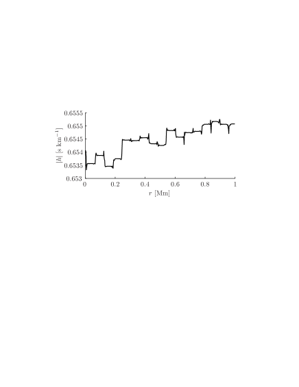
Figure 3: Hamiltonian $h$ vs. range for one of the scattered rays shown in Fig. 1b in the presence of an internal-wave-induced sound speed perturbation field.

For one of the rays used to produce Fig. 1, the Hamiltonian $h$ (whose numerical value is identical to that of $\bar{H}+\delta\bar{h}$, although they depend on different variables) as a function of range is shown in Fig. 3. It is seen that $h$ vs. $r$ consists of a sequence of approximately piecewise-constant segments, separated by fairly narrow transition regions. The transition regions coincide with each of the rays upper turning points. A useful and widely used approximation, the apex approximation, assumes that the width of each transition region is negligibly small. In the action–angle description of ray motion that makes use of the apex approximation, $I$ is piecewise constant following a ray, making jumps $\Delta I$ of negligibly small width $\Delta\vartheta$ at each upper turning depth of the ray; between such jumps $\vartheta$ advances by $2\pi.$ A slightly relaxed form of the apex approximation in which $\Delta\vartheta$ is treated as a small parameter will be used in Sec. IV. Generally, the apex approximation works fairly well in typical midlatitude deep ocean environments for rays with axial angles greater than about $10\unit{{{}^{\circ}}}$; it is usually a poor approximation for rays with axial angles less than approximately $5\unit{{{}^{\circ}}}.$ More generally, the apex approximation can be thought of as a special case of a scattering model in which $I$ is piecewise constant on a sequence of range intervals of variable extent. Such a model is used in Secs. III and IV. Although the apex approximation is a special case, it is useful to focus on this special case when considering constrained spreads because it is often the case Duda-etal-92 ; Worcester-etal-99 ; Colosi-etal-99 that only the steep ray travel time spreads can be measured experimentally.

III Unconstrained time spreads

A Spreading along the timefront

In this section we imagine launching rays from a fixed source location with a fixed launch angle in an ensemble of oceans, each with the same background sound speed structure, but with an independent realization of the internal-wave-induced perturbation field superimposed. At a fixed range we consider the resulting distribution of ray travel time perturbations without regard to the final ray depth or the ray turning point history. Such a distribution is seen in Fig. 1.

With the assumption that $I$ is piecewise constant following a ray, it follows from Eqs. (3), neglecting $\mathrm{d}\left(G-I\vartheta\right)/\mathrm{d}r$, that

$$\Delta T=\int_{0}^{r}\mathrm{d}\xi\,I(\xi)\omega^{\prime}(I(\xi))\Delta I(\xi).$$ (10)

Here, $\Delta T=T-T_{0},$ where $T_{0}(r)$ is the travel time of the unperturbed ray whose initial action is $I_{0};$ $\Delta I=I-I_{0}$; and $I$ and $\omega^{\prime}$ are understood to be piecewise constant functions of $r$. If the product $I\omega^{\prime}\approx I_{0}\omega^{\prime}(I_{0})$ over the domain of $I$-values assumed by the ray between ranges $0$ and $r,$ then (10) can be approximated by

$$\Delta T\approx I_{0}\omega^{\prime}(I_{0})\int_{0}^{r}\mathrm{d}\xi\,\Delta I(\xi).$$ (11)

Successive upper turns are typically separated by about $50$ km, which is large compared to the horizontal correlation length of internal-wave-induced sound speed fluctuations, so each perturbation to $I$ is independent. This leads to $\langle(\Delta I)^{2}\rangle^{1/2}\sim r^{1/2}$, where $\langle\cdot\rangle$ indicates ensemble average, and, in turn, to $\langle(\Delta T)^{2}\rangle^{1/2}\sim r^{3/2}.$ This $r^{3/2}$-dependence was previously derived by F. Henyey and J. Colosi (personal communication), who also found that this dependence is in good agreement with simulations. [Our simulations also indicate that when (11) is valid, then $\langle(\Delta T)^{2}\rangle^{1/2}\sim r^{3/2};$ our focus, however, is on the dependence of (10) and (7) on the background sound speed structure, via $I\omega^{\prime}$. We note, in addition, that if $\langle(\Delta I)^{2}\rangle^{1/2}$ is computed using an ensemble of rays with the same launch angle then the $r$-dependence of this quantity is characterized by oscillations in $r$ superimposed on the $r^{3/2}$ trend. The oscillations are caused by the cycling between relatively small time spreads when distributions are centered near the cusps where neighboring timefront branches join and relatively large time spreads when distributions are centered near the midpoint of timefront branches. At long range when scattered ray distributions are very broad, this effect is greatly dimished.] At long range the contributions to (10) or (11) from ray partial loops near the source and receiver are unimportant. Then, because $2\pi/\omega$ is the range of a ray double loop, for a ray that has undergone $N$ apex scattering events and has $N$ complete double loops, (11) can be further approximated,

$$\Delta T\approx 2\pi\frac{I_{0}\omega^{\prime}(I_{0})}{\omega(I_{0})}\sum_{i=1}^{N}(I_{i}-I_{0}).$$ (12)

Equation (12) provides an explanation for the observation (recall Fig. 1) that $\varphi_{0}=10^{\circ}$ rays in the C0 environment are more strongly scattered than $\varphi_{0}=12^{\circ}$ rays in the C14 environment; the same internal wave field was used to generate the ensemble of scattered rays, so the difference between these figures is due to the difference in the background sound speed profiles. The $\varphi_{0}=12^{\circ}$ rays in the C14 environment have a $|\omega^{\prime}(I_{0})|$-value that is approximately one-fourth that of the $\varphi_{0}=10^{\circ}$ rays in the C0 environment, and this scattering-induced time spread is seen to be reduced by a nearly commensurate amount, consistent with Eq. (12). According to that equation, travel time perturbations are the product of the amplification factor $I\omega^{\prime}/\omega$ and a term that depends on the history of the scattering-induced perturbations to the ray action variable.

It is convenient to introduce the stability parameter Abdullaev-Zaslavsky-91 ; Smirnov-Virovlyansky-Zaslavsky-01 ; Beron-Brown-03

$$\framebox{$\alpha=I\omega^{\prime}/\omega,$}$$ (13)

which, in addition to appearing in Eq. (12), is a natural nondimensional measure of $\omega^{\prime}.$ Figure 4 compares numerically simulated time spreads $\langle(\Delta T)^{2}\rangle^{1/2}$ as a function of launch angle $\varphi_{0}$ for a source on the sound channel axis at $r=2$ $\mathrm{Mm}$ to $\alpha$ in the two different background environments shown in Fig. 2 on which identical internal-wave-induced sound speed perturbation fields were superimposed. In the Fig. 4 plots, dependence on $I_{0}$ is replaced by dependence on the more familiar variable $\varphi_{0}$; for an axial source this constitutes a simple stretching of the horizontal axis. Ensembles of $\Delta T$ for rays with the same launch angle were generated using the same technique that was used to generate Fig. 1.

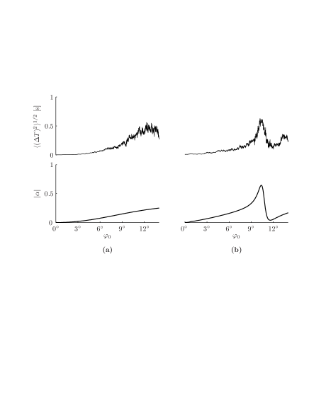
Figure 4: Estimates of unconstrained travel time spreads (upper panels) and the stability parameter $\alpha$ (lower panels) as a function of launch angle in background sound channels C0 (a) and C14 (b) (cf. Fig. 2). To generate the upper plots, ray simulations based on Eqs. (1) were performed by launching rays from a source located at the sound channel axis with a fixed launch angle in an ensemble of 50 oceans, each with the same background sound speed structure, but with an independent realization of the internal-wave-induced perturbation field superimposed.

Figure 4 shows that in both environments almost all of the structure seen in $\langle(\Delta T)^{2}\rangle^{1/2}$ can be attributed to the stability parameter $\alpha.$ This is because in the environments considered Eq. (12) is generally a good approximation to Eq. (10). Also, the dependence of $\sum_{i=1}^{N}(I_{i}-I_{0})$ on axial ray angle is somewhat weaker than the dependence of $\alpha$ on axial ray angle. We conclude from Fig. 4 that travel time spreads along the timefront are largely controlled by the background sound speed structure via $\alpha$, and that, provided $\alpha(I)$ does not have too much structure, the dependence of $\Delta T$ on $\alpha$ in Eq. (10) can be taken outside the integral.

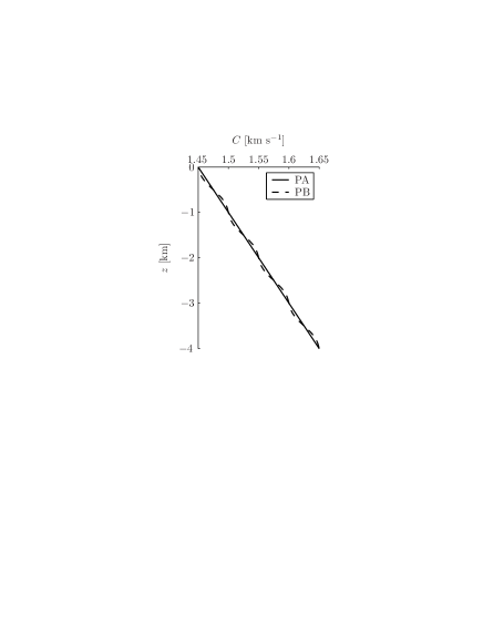
Figure 5: Background sound speed profiles used to construct the curves in Fig. 6.

B Spreading of rays with fixed turning history and final depth

We now consider a different measure of unconstrained travel time spread. To illustrate the generality of the results presented, we consider rays in upward refracting environments (Fig. 5) in the presence of rough surface scattering. In such environments the action–angle form of the ray equations is unchanged. The action $I$ is defined as in (6) with the upper turning depth $z_{+}=0$ for all rays. It follows from Eqs. (3), neglecting $\mathrm{d}\left(G-I\vartheta\right)/\mathrm{d}r$, that the travel time for one ray cycle is $T(I)=2\pi[I-\bar{H}(I)/\omega(I)].$ At each reflection from the rough surface the ray action gets modified. After $N$ surface reflections and $N+1$ ray cycles the travel time perturbation to the ray is

$$\Delta T_{N}\approx 2\pi\frac{\bar{H}(I_{0})\omega^{\prime}(I_{0})}{[\omega(I_{0})]^{2}}\sum_{i=1}^{N}(I_{i}-I_{0}),$$ (14)

where $I_{0}$ is the initial action of the ray, and the first of Eqs. (3a) has been used. Note that Eq. (14) constrains the ray geometry and final ray depth but not the final range of the scattered rays.

Figure 6 shows plots of $\Delta T_{20},$ defined in (14), vs. launch angle $\varphi_{0}$ for a source at the surface [so, again, $\varphi_{0}(I_{0})$ is a simple stretching] in the environments shown in Fig. 5. The rough surface was a single frozen realization of a surface gravity wavefield with a $k^{-7/2}$ surface elevation wavenumber spectrum with $0.02$ rad m${}^{-1}\leq k\leq 0.16$ rad m${}^{-1},$ $\Delta k=10^{-3}$ rad m${}^{-1},$ and an r.m.s. slope of $4\times 10^{-3}.$ Ray reflections from this surface were specular, but with a linearized boundary condition; the surface elevation was neglected, but the nonzero slope was not approximated. The same environments were used in Ref. Beron-Brown-03, .

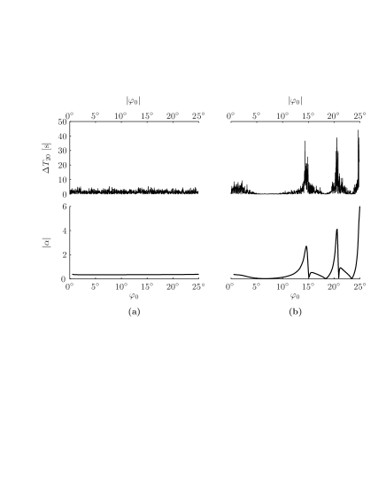
Figure 6: Upper panels: absolute value of the difference between perturbed (rough surface) and unperturbed (flat surface) ray travel time after 20 surface reflections as a function of initial ray angle at the surface for sound speed profiles PA (a) and PB (b) shown in Fig. 5. Lower panels: stability parameter as a function of ray angle in each of the two environments.

Consistent with Eq. (14), Fig. 6 shows that travel time perturbations are largely controlled by the background sound speed structure via $\alpha$, rather than details of the rough surface.

IV Constrained time spread

In this section we focus on deep ocean conditions and consider the scattering-induced broadening of an individual branch of the timefront. Note that this broadening is much smaller than the scattering-induced spreading along the timefront that was considered in section III.A. We refer to the broadening of an individual branch of the timefront as a constrained time spread because to calculate this broadening two constraints must be incorporated into the calculation. First, the rays contributing to the spread must have the same fixed endpoints in the $(z,r)$-plane. Second, the rays contributing to the spread must have the same turning point history, i.e. the same ray inclination (positive or negative) at the source, and the same number of turning points $M$ (upper and lower) between source and receiver. Note, however, that these constraints do not fix the values of the ray angle at either the source or receiver.

The approach taken here to compute appropriately constrained travel time spreads is based on a perturbation expansion that exploits the assumed smallness of the sound speed perturbation $\delta c$. The method by which the constraints are incorporated into the travel time perturbation estimates presented below is different than the method that was used in Ref. Beron-etal-03, ; that approach can be shown to give the same result that is presented below when terms of $O((\Delta I)^{2})$, neglecting endpoint corrections, are retained.

The perturbation expansions presented below make use of a scattering model in which $I$ following a scattered ray is piecewise constant; the apex approximation is then treated as a special case. Away form the scattering events Eqs. (3) are valid piecewise, with $I$ making a jump at each scattering event. Thus Eqs. (3) can be used to compute, in a piecewise fashion, the contribution of each ray segment to the travel time and range of the scattered ray. To impose the eigenray constraint, the total range of each scattered ray must be constrained to be equal to the range of the unperturbed ray. In addition, the turning point history, starting depth, and ending depth of the scattered ray must be the same as those of the unperturbed ray. This is accomplished by constraining the total change in $\vartheta$ following the scattered ray to be equal to that of the unperturbed ray. For some choices of the source–receiver geometry this procedure exactly enforces the eigenray constraint. In general, however, small endpoint corrections must be applied. For simplicity, these small endpoint corrections, which are important only at very short range, will be neglected.

We assume that between source and receiver the environment can be approximated as $n$ piecewice range-independent segments. Let $I_{i}$ denote the action of a scattered ray in the $i$th segment whose horizontal extent is $\Delta r_{i}=\Delta\vartheta_{i}/\omega(I_{i}),$ and let $\tilde{I}$ denote the action of the unperturbed ray. The eigenray constraint requires the perturbed ray total range, $r$, to be equal to the unperturbed ray total range. This condition reads

$$r=\sum_{i=1}^{n}\frac{\Delta\vartheta_{i}}{\omega(I_{i})}=\frac{1}{\omega(\tilde{I})}\sum_{i=1}^{n}\Delta\vartheta_{i},$$ (15)

which, for sufficiently small $\Delta I_{i}=I_{i}-\tilde{I}$, can be approximated by

$$\frac{\omega^{\prime}(\tilde{I})}{[\omega(\tilde{I})]^{2}}\sum_{i=1}^{n}\Delta I_{i}\Delta\vartheta_{i}=\frac{1}{2}\left.\frac{\mathrm{d}^{2}}{\mathrm{d}I^{2}}\right|_{I=\tilde{I}}\left(\frac{1}{\omega}\right)\sum_{i=1}^{n}(\Delta I_{i})^{2}\Delta\vartheta_{i}.$$ (16)

The r.h.s. term of (16) is almost always negligible compared to the l.h.s. term in deep ocean environments, even at ranges comparable to basin scales. Then, because $\Delta\vartheta_{i}=\omega(I_{i})\Delta r_{i}\approx\omega(\tilde{I})\Delta r_{i},$ the eigenray constraint reduces approximately to a statement that the range-weighted average of the perturbed action is equal to the unperturbed action, i.e.

$$\tilde{I}\approx r^{-1}\sum_{i=1}^{n}I_{i}\Delta r_{i}.$$ (17)

This equation constrains the action history of scattered eigenrays.

The difference between the perturbed and unperturbed ray travel times is

$$\Delta T = \sum_{i=1}^{n}\left[I_{i}-\frac{\bar{H}(I_{i})}{\omega(I_{i})}\right]\Delta\vartheta_{i}-\left[\tilde{I}-\frac{\bar{H}(\tilde{I})}{\omega(\tilde{I})}\right]\sum_{i=1}^{n}\Delta\vartheta_{i}$$ (18)

$$\approx \frac{\omega^{\prime}(\tilde{I})\bar{H}(\tilde{I})}{[\omega(\tilde{I})]^{2}}\sum_{i=1}^{n}\Delta I_{i}\Delta\vartheta_{i}-\frac{1}{2}\left.\frac{\mathrm{d}^{2}}{\mathrm{d}I^{2}}\right|_{I=\tilde{I}}\left(\frac{\bar{H}}{\omega}\right)\sum_{i=1}^{n}(\Delta I_{i})^{2}\Delta\vartheta_{i}$$

$$= \frac{1}{2}\frac{\omega^{\prime}(\tilde{I})}{\omega(\tilde{I})}\sum_{i=1}^{n}(\Delta I_{i})^{2}\Delta\vartheta_{i},$$

where the eigenray constraint (16) has been used. Virovlyansky Virovlansky-03 recently derived an expression for $\Delta T$ consisting of Eq. (18) [written as an integral over $r$ using $\Delta\vartheta_{i}=\omega(I_{i})\Delta r_{i}$] plus a correction term. We will discuss his result in more detail below. It should also be noted that the same symbol $\Delta T$ is being used to denote a constrained (eigenray) travel time perturbation that was used in the previous section to denote an unconstrained travel time perturbation. We believe that is obvious in all cases which is the relevant quantity. This choice was made to keep the notation simple. Also, for the same reason, we make no notational distinction between a theoretical estimate of $\Delta T$ and a numerically computed $\Delta T.$

The apex approximation is a special case of the analysis leading to Eqs. (15)-(18). If the contributions to $\Delta T$ from the incomplete ray cycles at the beginning and end of the ray path are neglected, Eq. (18) applies with $\Delta\vartheta_{i}=2\pi$ and $n=N,$ the number of complete ray cycles. (For large $N$ the neglected incomplete ray cycle contributions to $\Delta T$ constitute small corrections to the sum of the retained contributions.)

In Ref. Beron-etal-03, a relaxed form of the apex approximation was considered. The transition width of the jump $\Delta I_{\mathrm{T}}=I_{i}-I_{i-1}$ had a width $\Delta\vartheta_{\mathrm{T}},$ which is assumed here to be small, $\Delta\vartheta_{\mathrm{T}}<2\pi.$ In the transition region a particular form $\bar{h}(I-\vartheta\Delta I_{\mathrm{T}}/\Delta\vartheta_{\mathrm{T}})$ of the Hamiltonian was assumed. This finite width transition region was shown not to contribute to a range perturbation, but gives a travel time perturbation $\frac{1}{2}\Delta I_{\mathrm{T}}\Delta\vartheta_{\mathrm{T}}$ for a single scattering event. After $N$ scattering events, assuming the transition width $\Delta\vartheta_{\mathrm{T}}$ of each is the same, this gives a contribution $\frac{1}{2}(I_{N}-I_{0})\Delta\vartheta_{\mathrm{T}}$ to $\Delta T$ (18), while the eigenray constraint (16) is unaltered. With this additional term (18), with $\Delta\vartheta_{i}=2\pi$ and $n=N,$ is replaced by

$$\Delta T=\dfrac{1}{2}(I_{N}-I_{0})\Delta\vartheta_{\mathrm{T}}+\pi\frac{\omega^{\prime}(\tilde{I})}{\omega(\tilde{I})}\sum_{i=1}^{N}(\Delta I_{i})^{2}.$$ (19)

For convenience we shall refer to the first and second terms on the r.h.s. of Eq. (19) as $\Delta T_{1}$ and $\Delta T_{2},$ respectively. For steep rays in typical deep ocean environments $\Delta\vartheta_{\mathrm{T}}/(2\pi)\approx 0.05$ while $\omega^{\prime}\Delta I_{\mathrm{T}}/\omega\approx 0.01.$ (The latter estimate is variable owing to variations in $\omega^{\prime}.$) Thus one might expect that $\Delta T_{1}$ dominates $\Delta T_{2}$. For small $N$ this is indeed the case. But under typical deep ocean conditions consecutive apex scattering events are independent (because the ray cycle distance $2\pi/\omega\approx 50$ km exceeds the horizontal correlation length of internal waves, about $10$ km), so $\Delta T_{1}$ and $\Delta T_{2}$ grow approximately like $N^{1/2}$ and $N,$ respectively. Thus $\Delta T_{2}$ is expected to dominate $\Delta T_{1}$ at long range. Note that when $\Delta T_{2}$ dominates $\Delta T_{1}$, this equation predicts a scattering-induced travel time bias in the direction of $\mathop{\mathrm{s}gn}\omega^{\prime}.$

Figure 7: (a) Ray travel time and depth of rays with positive launch angles and which have $N=18$ upper turning points at $r=1$ Mm in the C0 environment shown in Fig. 2. The solid curve correponds to rays in the absence of internal-wave-induced scattering. Dots correspond to rays scattered by internal waves. (b) Same as the left panel except that $r=3$ Mm and $N=54.$

These observations are consistent with the simulations shown in Fig. 7. There, scattered and unperturbed ($\delta c=0$) ray travel times are shown in the vicinity of two branches of the timefront at $r=1$ $\mathrm{Mm}$ ($N=18$) and $r=3$ $\mathrm{Mm}$ ($N=54$). At both ranges the source was on the sound channel axis in the C0 environment shown in Fig. 2; launch angles for the rays shown are near $10^{\circ}$ at both ranges. In that environment $\mathop{\mathrm{s}gn}\omega^{\prime}=-1.$ It is seen in this figure that there is no indication of a negative travel time bias at $1$ $\mathrm{Mm}$, while there is a clear negative bias at $3$ $\mathrm{Mm}$, consistent with Eq. (19). At ranges sufficiently short that $\Delta T_{1}$ dominates, travel time biases of either sign can be expected as $I_{N}-I_{0}$ can be of either sign. Because $I_{N}-I_{0}$ is a continuous function of launch angle, such biases should have a nonzero correlation scale along the timefront. These features are readily evident in our simulations in the presence of realistic internal-wave-induced sound speed perturbations.

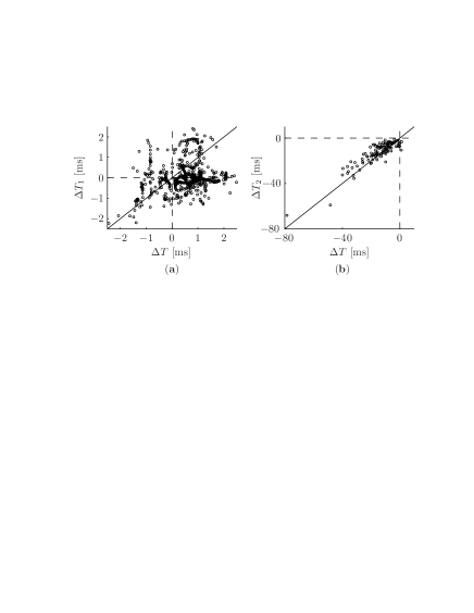
Figure 8: (a) Constrained travel time spread ($\Delta T$) vs. the first term on the r.h.s. of Eq. (19) ($\Delta T_{1}$) at $r=500$ km for rays with axial launch angles $11^{\circ}\leq\varphi_{0}\leq 13.5^{\circ}$ in the C0 environment with an internal-wave-induced sound speed perturbation superimposed. (b) As in (a) but vs. the second term on the r.h.s. of Eq. (19) ($\Delta T_{2}$) and at $r=3$ Mm.

Quantitative tests of the correctness of Eq. (19) are shown in Fig. 8. There numerically computed travel time differences $\Delta T$ are compared separately to $\Delta T_{1}$ and $\Delta T_{2}$ under conditions in which one of the two terms dominates the other. The constrained travel time difference $\Delta T$ was computed using a single realization of an internal-wave-induced sound speed perturbation as the difference between the perturbed ray with the same turning history and the same final depth as the unperturbed ray. In Fig. 8 attention is restricted to rays that are sufficiently steep that the apex approximation is approximately valid, but not so steep that rays reflect off the surface.

In Fig. 8a $\Delta T$ is compared to $\Delta T_{1}$ at $r=500$ km; for the rays used to construct this plot the mean value of $\Delta T_{2}$ is $-0.3$ ms, which is seen to represent a small correction, on average, to $\Delta T_{1}.$ The value of $\Delta\vartheta_{\mathrm{T}}$ used to construct this plot is $0.25\approx 2\pi/25.$ The domain and gross distribution of $\Delta T$ points plotted in Fig. 8a is seen to coincide with the domain and gross distribution of $\Delta T_{1}$ points plotted. Thus $\Delta T_{1}$ is a fairly good statistical descriptor of $\Delta T$. The point-by-point comparison between $\Delta T$ and $\Delta T_{1}$ is not good, however. This is seen by noting that the points plotted do not cluster along the diagonal line with slope unity. Thus, although $\Delta T_{1}$ has the correct qualitative features and appears to be a useful statistical descriptor of $\Delta T,$ it is evidently a poor deterministic predictor of $\Delta T.$ This shortcoming, we believe is attributable to the overly idealized form of the Hamiltonian in the apex transition region that was used to derive $\Delta T_{1}.$ It is interesting to note that $\Delta T_{1}$ is the only term presented in this paper describing a travel time spread that is independent of $\omega^{\prime},$ and this term is the one that gives the poorest agreement with simulations.

In Fig. 8b $\Delta T$ is compared to $\Delta T_{2}$ at $r=3$ Mm; for the rays used to construct this plot the r.m.s. value of $\Delta T_{1}$ is $2$ ms, which is seen to represent a small correction, on average, to $\Delta T_{2}.$ The agreement between $\Delta T$ and $\Delta T_{2}$ in this plot is seen to be very good, indicating that for the rays used to construct this plot $\Delta T_{2}$ is a very good predictor of $\Delta T.$ Overall, for steep rays we have found good qualitative agreement at short range between simulations of $\Delta T$ and $\Delta T_{1}$, and a good quantitative agreement at long range between $\Delta T$ and $\Delta T_{2}.$

Figure 9 shows plots of $\Delta T$ vs. launch angle and $\alpha$ vs. launch angle at $r=3$ Mm in each of the two background sound speed profiles shown in Fig. 2. Again, the constrained travel time spread $\Delta T$ was computed using a single realization of an internal-wave-induced sound speed perturbation as the difference between the perturbed ray travel time and the travel time of the unperturbed ray with the same turning history and the same final depth as the perturbed ray. The small gaps in the plot correspond to perturbed rays whose final depth lies outside the bounds of the portion of the timefront which has the same turning history as the perturbed ray. In Fig. 9 ray angles are not limited to the band for which the apex approximation is expected to be valid. Thus Eq. (19) is not expected to be valid for the entire band of angles. Equation (18) should be approximately valid across the entire band, however, so the trend in $\alpha(\varphi_{0})$ should be approximately reproduced in the $\Delta T(\varphi_{0})$ points plotted. This is seen to be the case; variations in $\Delta T$ are caused by variations in $\sum_{i=1}^{n}(\Delta I_{i})^{2}\Delta\vartheta_{i}$. The probable cause of the positive values of $\Delta T$ for near-axial rays in the C0 environment seen in Fig. (9) will be discussed below. Even after fitting a smooth curve through the fluctuations seen in the Fig. 9 $\Delta T$ plot for the C14 environment, the peak in $|\Delta T|$ is seen to be less pronounced than the peak in $|\alpha|.$ This is expected because the scattering process leads to a local average over a band of adjacent $\alpha$-values. With these minor caveats, Fig. 9 shows that constrained travel time spreads at long range are largely controlled by the background sound speed structure via the stability parameter $\alpha.$ The same conclusion can be drawn from Fig. 8b.

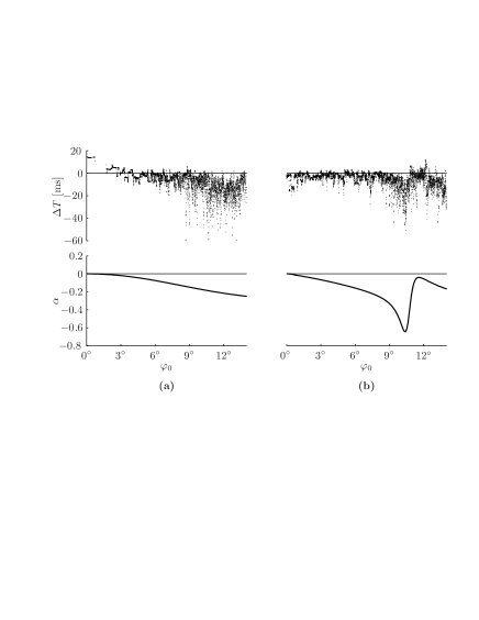
Figure 9: Travel time difference $\Delta T=T_{\mathrm{IW}}-T_{0}$ at $r=3$ Mm vs. ray launch angle $\varphi_{0}$ for an axial source, and stability parameter $\alpha$ vs. $\varphi_{0},$ in each of the environments C0 (a) and C14 (b) shown in Fig. 2. Here, $T_{\mathrm{IW}}$ is the travel time of a ray in the presence of an internal-wave-induced sound speed perturbation field, and $T_{0}$ is the travel of a ray in the same background environment, but without the sound speed perturbation field superimposed, whose turning point history and final depth are the same as those of the $T_{\mathrm{IW}}$ ray.

The probable cause of the positive computed values of $\Delta T$ for near-axial rays seen in Fig. 9 in the C0 environment is not the failure of Eq. (19); rather it is the failure of our ray labeling scheme for near axial rays. We have implicitly assumed that the ray identifier $\pm M$ uniquely identifies each timefront branch. This assumption fails for near-axial rays. (The assumption also fails for steep rays in the vicinity of the cusps where adjacent timefront branches join, and whenever $\omega^{\prime}$ has isolated zeros. We have intentionally avoided the latter situation.) The correct way to identify timefront branches is by the Maslov index Brown-etal-03 $\mu$ which, for waves in two space dimensions, advances by one unit each time a caustic is touched. For near-axial rays the portion of the timefront corresponding to a constant value of the ray identifier consists of two adjacent partial branches joined at a cusp. For these rays a ray-identifier-based definition of $\Delta T$ can lead to either undefined or nonuniquely defined $\Delta T$ values.

We noted earlier the quantitative correctness of $\Delta T_{2}$ and the qualitative correctness of $\Delta T_{1}.$ The weakest link in our analysis is clearly $\Delta T_{1}.$ Virovlyansky Virovlansky-03 derived an alternate correction to $\Delta T_{2}$ whose validity, like (18), is not linked to the apex approximation. In our notation, this correction reads

$$\Delta T_{1}^{\mathrm{V}} = \int_{0}^{r}\mathrm{d}\xi\,\Delta I(\xi)\frac{\partial\delta\bar{h}}{\partial I}(I(\xi),\vartheta(\xi),\xi)$$ (20)

$$-\int_{0}^{r}\mathrm{d}\xi\,\delta h(p(\xi),z(\xi),\xi).$$

Unfortunately, the lack of explicit knowledge on the functional dependence of $\delta\bar{h}$ on $(I,\vartheta,r)$ makes the numerical evaluation of the first term on r.h.s. of (20) quite difficult—if not impossible. Virovlyansky argued that that term can be neglected. We have evaluated numerically the second term on r.h.s. of (20); this resulted in significantly poorer agreement with our simulations that was found using our $\Delta T_{1}$. (Note, however, that the parameter $\Delta\vartheta_{\mathrm{T}}$ in our expression for $\Delta T_{1}$ was adjusted to approximately match the simulations.) We expect, but have not confirmed, that the evaluation of both terms on the r.h.s. of (20) would result in good agreement with simulations.

V Discussion and conclusions

In this paper we have investigated three measures of travel time spreads for sound propagation in environments consisting of a range independent background on which a range-dependent perturbation is superimposed: (i) unconstrained spread of ray travel time along the timefront; (ii) unconstrained spread of rays whose turning history and final depth are fixed but whose final range is not; and (iii) scattering-induced broadening of an individual branch of the timefront at a fixed location. All three measures of time spreads were shown to be largely controlled by a property $\omega^{\prime}$ of the background sound speed profile. Surprisingly, this is the same property that controls ray spreading and, hence, ray amplitudes Beron-Brown-03 . We now present two arguments that provide some insight into why travel time spreads should be controlled by the same property of the background sound speed profile that controls ray spreading.

The variational equations that describe how small perturbations $(\delta I,\delta\vartheta,\delta T)$ evolve in the extended phase space $(I,\vartheta,T)$ are given by

$$\frac{\mathrm{d}}{\mathrm{d}r}\left(\begin{array}[]{c}\delta I\\ \delta\vartheta\\ \delta T\end{array}\right)=\left[\begin{array}[]{ccc}-\delta\bar{h}_{,I\vartheta}&\delta\bar{h}_{,\vartheta\vartheta}&0\\ \omega^{\prime}+\delta\bar{h}_{,II}&\delta\bar{h}_{,I\vartheta}&0\\ I\omega^{\prime}+I\delta\bar{h}_{,II}&I\delta\bar{h}_{,I\vartheta}-\delta\bar{h}_{,\vartheta}&0\end{array}\right]\left(\begin{array}[]{c}\delta I\\ \delta\vartheta\\ \delta T\end{array}\right),$$ (21)

where a short-hand notation for partial differentiation has been introduced. In general Eqs. (21) and (7) constitute a set of six coupled differential equations. For the special case $\delta\bar{h}=0,$ $I$ and $\omega^{\prime}$ are constant following trajectories and (21), like (7), have a simple analytical solution. For the class of problems treated in this paper the nonzero sound speed perturbation terms in the matrix on the r.h.s. of (21) are generally much smaller than the $\omega^{\prime}$ and $I\omega^{\prime}$ terms, corresponding to contributions from the background sound speed profile. Thus one expects that generically the dominant cause of the growth of $(\delta I,\delta\vartheta,\delta T)$ is the background sound speed structure via $\omega^{\prime},$ rather than the small sound speed perturbation terms. Loosely speaking, the perturbation terms provide a seed for the growth of $(\delta I,\delta\vartheta,\delta T),$ while subsequently growth of these quantities is largely controlled by $\omega^{\prime}.$

Additional insight into the role played by $\omega^{\prime}$ is obtained by making a fluid mechanical analogy. Equations (1) define a flow in the three-dimensional space $(p,z,T)$ with velocity components $\mathrm{d}(p,z,T)/\mathrm{d}r.$ (Recall that $r$ plays the role of the independent or time-like variable in the one-way ray equations.) Alternatively, the flow in this three-dimensional space can be described using action–angle variables $(I,\vartheta,T).$ The coordinates $(I,\vartheta,T)$ behave qualitatively like cylindrical coordinates $(\rho,\theta,\zeta)$, say. If we neglect the contributions from the sound speed perturbation term $\delta\bar{h},$ then the velocity components of the background flow in these coordinates are $u_{I}=\mathrm{d}I/\mathrm{d}r=0,$ $u_{\vartheta}=(\mathrm{d}\vartheta/\mathrm{d}r)I=\omega I,$ and $u_{T}=\mathrm{d}T/\mathrm{d}r=I\omega-\bar{H}.$ The strain rate tensor,

$$\mathsf{S}_{j}^{i}:=\tfrac{1}{2}\left(\nabla_{j}u^{i}+\nabla_{i}u^{j}\right),$$ (22)

where $\nabla_{i}$ denotes covariant derivative, describes how small elements of fluid are deformed by the flow Batchelor-64 . With the identification $(I,\vartheta,T)\leftrightarrow(\rho,\theta,\zeta)$ and with the velocity field $(u_{I},u_{\vartheta},u_{T})$ defined above, the strain rate tensor is

$$\mathsf{S}=\left[\begin{array}[]{ccc}0&\frac{1}{2}I\omega^{\prime}&\frac{1}{2}I\omega^{\prime}\\ \frac{1}{2}I\omega^{\prime}&0&0\\ \frac{1}{2}I\omega^{\prime}&0&0\end{array}\right].$$ (23)

Although (23) is only qualitatively correct [because of the qualitative connection between $(I,\vartheta,T)$ and $(\rho,\theta,\zeta)$], the conclusion to be drawn from this tensor is extremely important: deformation of small elements of the extended phase space $(I,\vartheta,T)$ by the background sound speed structure is caused entirely by shear (off-diagonal elements of $\mathsf{S}$) and is quantified by the product $I\omega^{\prime}.$ This behavior is consistent with the discussion above concerning Eq. (21) and the growth of small perturbations in the extended phase space $(I,\vartheta,T).$

Arguments similar to those given above relating to Eqs. (21) and (23) were given in Ref. Beron-Brown-03, ; in that study, however, attention was confined to ray spreading in $(p,z)$ or, equivalently, $(I,\vartheta).$ That problem is described by the first two of Eqs. (1) or (7), the upper $2\times 2$ system in Eqs. (21) and (23), etc. In that study it was shown that ray spreading is largely controlled by $\omega^{\prime}.$ The surprising result of the present study is that travel time spreads are also largely controlled by $\omega^{\prime}.$ This is evident from the unconstrained and constrained travel time spread estimates, (10), (14), (18), and (19), and the more heuristic arguments associated with Eqs. (21) and (23).

Inasmuch as the AET experimental observations Worcester-etal-99 ; Colosi-etal-99 provided much of the motivation for the present work, it is noteworthy that the results presented here are consistent with the ray-based analysis of those observations presented in Ref. Beron-etal-03, . Two points relating to the results in Ref. Beron-etal-03, deserve further comment. First, it was argued in Ref. Beron-etal-03, that, for moderately steep rays, constrained travel time spreads could be approximately estimated using $\Delta T_{1},$ the first term on the r.h.s. of Eq. (19). This is moderately surprising in that the AET range was $3.25$ Mm, which is large enough that one would expect that the second term on r.h.s. of (19) should be important. The neglected term, however, is proportional to $\alpha$, which is unusually small (cf. Ref. Beron-etal-03, ) in that environment for the relevant band of launch angles. Thus the estimated travel time spread reported in Ref. Beron-etal-03, is close to what one obtains using both terms on the r.h.s. of Eq. (19). Second, it was noted in Ref. Beron-etal-03, , without explanation, that in the AET environment constrained travel time spreads are much larger for near axial rays than for steeper rays. This behavior is consistent with Eq. (18) and the observation Beron-etal-03 that in the AET environment $\left|\alpha\right|$ is very large for the near-axial rays.

The results presented in this paper, coupled with those presented in Refs. Beron-Brown-03, ; Virovlansky-03, , represent an important step toward the development of a theory of wave propagation in random inhomogeneous media (WPRIM). These studies have shown that both ray amplitude statistics and ray travel time statistics are largely controlled by the background sound speed profile, via $\omega^{\prime}.$ It follows that finite frequency wavefield intensity statistics should also be largely controlled by the background sound speed profile via $\omega^{\prime}.$ This is different from the classical treatment of the problem of wave propagation in random media (WPRM) which assumes that the background sound speed structure is homogeneous—for which $\omega^{\prime}=0.$ Ideally one would like to develop a uniformly valid theory of WPRIM that reduces to known WPRM results in the limit $\omega^{\prime}\rightarrow 0.$ A more modest goal is to develop an approximate theory of WPRIM, appropriate for long-range underwater sound propagation, that treats the case where the wavefield intensity statistics are largely controlled by $\omega^{\prime}.$ To develop such a theory the results presented here and in Refs. Beron-Brown-03, ; Virovlansky-03, have to be combined and extended. Necessary extensions are the inclusion of finite frequency effects (interference and diffraction) and a more accurate treatment of the link between sound speed perturbations and perturbations to $I$ and $\vartheta.$ These topics will be explored in future work.

References

- (1) T. F. Duda, S. M. Flatté, J. A. Colosi, B. D. Cornuelle, J. A. Hildebrand, W. S. Hodgkiss, P. F. Worcester, B. M. Howe, J. A. Mercer, and R. C. Spindel, “Measured wavefront fluctuations in 1000 km pulse propagation in the Pacific Ocean,” J. Acoust. Soc. Am. 92, 939–955 (1992).
- (2) P. F. Worcester, B. D. Cornuelle, M. A. Dzieciuch, W. H. Munk, J. A. Colosi, B. M. Howe, J. A. Mercer, A. B. Baggeroer, and K. Metzger, “A test of basin-scale acoustic thermometry using a large-aperture vertical array at 3250-km range in the eastern North Pacific Ocean,” J. Acoust. Soc. Am. 105, 3,185–3,201 (1999).
- (3) J. A. Colosi, E. K. Scheer, S. M. Flatté, B. D. Cornuelle, M. A. Dzieciuch, W. H. Munk, P. F. Worcester, B. M. Howe, J. A. Mercer, R. C. Spindel, K. Metzger, and T. Birdsall, “Comparison of measured and predicted acoustic fluctuations for a 3250-km propagation experiment in the eastern North Pacific Ocean,” J. Acoust. Soc. Am. 105, 3,202–3,218 (1999).
- (4) T. F. Duda and J. B. Bowlin, “Ray-acoustic caustic formation and timing effects from ocean sound-speed relative curvature,” J. Acoust. Soc. Am. 96, 1,033–1,046 (1994).
- (5) J. Simmen, S. M. Flatté, and G. Yu-Wang, “Wavefront folding, chaos and diffraction for sound propagation through ocean internal waves,” J. Acoust. Soc. Am. 102, 239–255 (1997).
- (6) I. P. Smirnov, A. L. Virovlyansky, and G. M. Zaslavsky, “Theory and application of ray chaos to underwater acoustics,” Phys. Rev. E 64, 036221, 1–20 (2001).
- (7) F. J. Beron-Vera and M. .G. Brown, “Ray stability in weakly range-dependent sound channels,” J. Acoust. Soc. Am. (2003), in press.
- (8) M. G. Brown, J. A. Colosi, S. Tomsovic, A. L. Virovlyansky, M. Wolfson, and G. M. Zaslavsky, “Ray dynamics in long-range deep ocean sound propagation,” J. Acoust. Soc. Am. (2003), in press.
- (9) W. H. Munk, “Sound channel in an exponentially stratified ocean with application to SOFAR,” J. Acoust. Soc. Am. 55, 220–226 (1974).
- (10) F. J. Beron-Vera, M. G. Brown, J. A. Colosi, S. Tomsovic, A. L. Virovlyansky, M. A. Wolfson, and G. M. Zaslavsky, “Ray dynamics in a long-range acoustic propagation experiment,” J. Acoust. Soc. Am. (2003), conditionally accepted.
- (11) J. A. Colosi and M. G. Brown, “Efficient numerical simulation of stochastic internal-wave-induced sound speed perturbation fields,” J. Acoust. Soc. Am. 103, 2,232–2,235 (1998).
- (12) G. K. Batchelor, An Introduction to Fluid Dynamics (Cambridge University, 1964).
- (13) M. G. Brown and J. Viechnicki, “Stochastic ray theory for long-range sound propagation in deep ocean environments,” J. Acoust. Soc. Am. 104, 2,090–2,104 (1998).
- (14) A. L. Virovlyansky, “Ray travel times at long range in acoustic waveguides,” J. Acoust. Soc. Am. 113, 2,523–2,532 (2003).
- (15) V. I. Arnold, Mathematical Methods of Classical Mechanics, 2nd edn. (Springer, 1989).
- (16) L. D. Landau and E. M. Lifshitz, Mechanics, 3rd edn. (Pergamon, 1976).
- (17) S. S. Abdullaev and G. M. Zaslavsky, “Classical nonlinear dynamics and chaos of rays in problems of wave propagation in inhomogeneous media,” Usp. Fiz. Nauk 161, 1-43 (1991).