On dissipationless shock waves in a discrete nonlinear Schrödinger equation

Abstract

It is shown that the generalized discrete nonlinear Schrödinger equation can be reduced in a small amplitude approximation to the KdV, mKdV, KdV(2) or the fifth-order KdV equations, depending on values of the parameters. In dispersionless limit these equations lead to wave breaking phenomenon for general enough initial conditions, and, after taking into account small dispersion effects, result in formation of dissipationless shock waves. The Whitham theory of modulations of nonlinear waves is used for analytical description of such waves.

PACS numbers: 05.45.Yv, 05.90.+m

I Introduction

Dissipationless shock waves have been experimentally observed or their existence has been theoretically predicted in various nonlinear media – water Whitham74 , plasma Sagdeev64 , optical fibers Krokel , lattices lattice . In contrast to usual dissipative shocks where combined action of nonlinear and dissipation effects leads to sharp jumps of the wave intensity, accompanied by abrupt changes of other wave characteristics, in dissipationless shocks the viscosity effect is negligibly small compared with the dispersive one, and, instead of intensity jumps, the combined action of nonlinear and dispersion effects leads to formation oscillatory wave region (for review see e.g. kamch2000 ). Since intrinsic discreteness of a solid state system gives origin to strong dispersion, which can dominate dissipative effects in wave phenomena, it is of considerable interest to investigate details of formation of dissipationless shocks in lattices.

As a model, in the present paper we choose the general discrete nonlinear Schrödinger (GDNLS) equation

$$i\dot{q}_{n}+(1-\eta|q_{n}|^{2})(q_{n+1}+q_{n-1}-2q_{n})+2(\rho^{2}-|q_{n}|^{2})q_{n}=0$$ (1)

introduced by Salerno Salerno92a ; ESSE92 . Eq. (1) turned out to be an important model not only because of its property to provide a one-parametric transition between an integrable Ablowitz-Ladik (AL) model and the so-called discrete nonlinear Schrödinger (DNLS) equation ($\eta=1$ and $\eta=0$, respectively), but also because of a number of physical application for a review of which we refer to Hennig .

Obviously, (1) has a constant amplitude solution $q_{n}=\rho$. It was shown in KS97a ; KS97b , that in a small amplitude, $|a|\ll\rho$, and long wave (so that the discrete site index $n$ can be replaced by a continuous coordinate $x$) limit, evolution of small amplitude perturbations with respect to this constant background,

$$q_{n}(t)=(\rho+a(x,t))\exp(-i\phi(x,t)),$$ (2)

is governed by the Korteweg-de Vries (KdV) equation for the amplitude $a(x,t)$:

$$a_{t}-\frac{2(3-4\eta\rho^{2})}{\sqrt{1-\eta\rho^{2}}}aa_{x}+\frac{\sqrt{1-\eta\rho^{2}}}{12\rho}[3(1-\eta\rho^{2})-\rho^{2}]a_{xxx}=0$$ (3)

which is written in the reference system moving with velocity $2\rho\sqrt{1-\eta\rho^{2}}$ of linear waves in dispersionless limit. It is well known (see, e.g. Whitham74 ) that if the initial pulse is strong enough, so that the nonlinear term dominates over the dispersive one at the initial stage of the pulse evolution, then the dissipationless shock wave develops after the wave breaking point. The theory of such waves, described by the KdV equation, is well developed (see, e.g. kamch2000 ). Existence of the respective shock waves for model (1) has been predicted analytically and observed in numerical simulations in KS97a ; KS97b . Moreover, as it is shown in KonChaos a nonlinear Schrödinger equation of a rather general type can bear “KdV-type” shock waves. In this context the results presented below in the present paper although being mostly related to model (1) display some general characteristic features of a lattice of a nonlinear Schrödinger type.

The coefficients of (3) depend on two parameters $\eta$ and $\rho$ and can vanish at special choice of these parameters, so the KdV equation looses its applicability for these values of $\eta$ and $\rho$. Physically acceptable values of $\eta$ and $\rho$ are limited by the inequalities

$$0\leq\eta\leq\mathrm{min}\{1,1/\rho^{2}\},\quad 0<\rho<\infty,$$ (4)

and this region of the $(\rho,\eta)$ plane is depicted in Fig. 1.

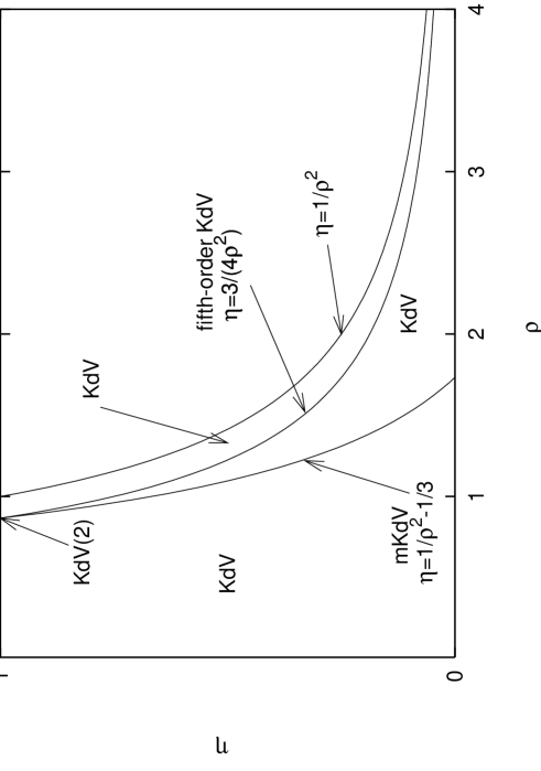
Figure 1: Diagram showing different continuous limits of the GDNLS equation. The abbreviations are explained in the text.

Along the line

$$\eta=\frac{3}{4\rho^{2}}$$ (5)

the coefficient before the nonlinear term in (3) vanishes. This means that implied in derivation of the KdV equation approximation limited to only quadratic nonlinearities fails and higher nonlinearities have to be taken into account for accurate description of the wave dynamics. Hence, one may expect that the modified KdV (mKdV) equation with cubic nonlinearity arises for values of $\rho$ and $\eta$ related by (5).

Along the line

$$\eta=\frac{1}{\rho^{2}}-\frac{1}{3}$$ (6)

the coefficient before the dispersion term in (3) vanishes what means that higher order dispersion effects have to be taken into account. In this case one may expect that evolution equation for $a(x,t)$ contains quadratic nonlinear term and linear dispersion term with fifth-order space derivative of $a(x,t)$.

The most interesting point corresponds to the values

$$\eta=1,\quad\rho=\sqrt{3}/2$$ (7)

when both nonlinear and dispersion coefficients vanish. Since Eq. (1) with $\eta=1$ coincides with the completely integrable Ablowitz-Ladik equation, one may expect that in a small amplitude approximation this equation with the parameters equal to (7) reduces again to a completely integrable equation. The KdV equation (3) with $\eta=1$ is valid for all interval $0<\rho<1$ except for some vicinity of the point $\rho=\sqrt{3}/2$, and therefore one can suppose that at the point (3) one has to obtain the second equation of the KdV hierarchy KdV(2) in which the higher order nonlinear and dispersion effects play the dominant role.

The aim of this paper is two-fold. At first, in Sec. II we derive the evolution equations for the whole region (4) and show that along the line (5) the small-amplitude approximation reduces to the mKdV equation (Sec II.2), along the line (6) to a nonlinear equation with the dispersion of the fifth-order (Sec II.3), and at the point (7) to the KdV(2) equation (Sec II.4). The last result sheds some new light on the nature of higher equations of the KdV hierarchy—they arise as small amplitude approximations to completely integrable equations, if lower orders of nonlinear and dispersion contributions vanish at some values of the parameters of the equation under consideration.

The second aim of the paper is to develop a theory of shock waves (Sec III) for the mKdV (Sec III.1)and KdV(2) (Sec III.2) equations analogous to that developed earlier for the KdV equation. This theory permits one to described in details the behavior of shocks after the wave breaking point for different values of the parameters entering into Eq. (1). The results are summarized in Conclusion.

II Small amplitude approximation

Using ansatz (2) and replacing a discrete index $n$ by a continuous variable $x$, we rewrite Eq. (1) as

$$\begin{split}ia_{t}+(\rho+a)\phi_{t}-4\rho^{2}a-6\rho a^{2}+[1-\eta(\rho+a)^{2}]\\ \times\{(\rho+a(x+1,t))\exp[-i(\phi(x+1,t)-\phi(x,t))]\\ +(\rho+a(x-1,t))\exp[-i(\phi(x-1,t)-\phi(x,t))]\}=0.\end{split}$$ (8)

In the linear approximation, this equation yields for the harmonic wave solution

$$a(x,t)\propto\exp[i(Kx-\Omega t)],\quad\phi(x,t)\propto\exp[i(Kx-\Omega t)],$$

the dispersion relation KS97a ; KS97b

$$\begin{split}\Omega=\pm 4\sqrt{1-\eta\rho^{2}}\sin\frac{K}{2}\left[\rho^{2}+(1-\eta\rho^{2})\sin^{2}\frac{K}{2}\right]^{1/2}\\ \cong\pm 2\rho\sqrt{1-\eta\rho^{2}}\,K\cdot\left[1+\frac{3(1-\eta\rho^{2})-\rho^{2}}{24\rho^{2}}\,K^{2}+O(K^{4})\right],\end{split}$$ (9)

where expansion in powers of $K$ corresponds to taking into account different orders of the dispersion effects. In the lowest order, when the dispersion effects are neglected, linear waves propagate with constant velocity

$$v=\pm 2\rho\sqrt{1-\eta\rho^{2}}.$$ (10)

To evaluate contribution of small (for $|a|\ll\rho$) nonlinear effects, it is convenient to introduce a small parameter $\varepsilon\sim a$ and pass to such scaled variables in which nonlinear and dispersion effects make contributions of the same order of magnitude into evolution of the wave. Since the choice of these scaled variables depends on values of the parameters, we shall consider the relevant cases separately.

II.1 KdV equation

For the sake of completeness we start by reproducing briefly some results of KS97a . We expand $a(x\pm 1,t)$ and $\phi(x\pm 1,t)$ into the Taylor series around $x$, introduce scaling indexes

$$a\sim\varepsilon,\quad t\sim\varepsilon^{-\alpha},\quad x\sim\varepsilon^{-\beta},\quad\phi\sim\varepsilon^{\gamma},$$ (11)

and demand that in the reference frame moving with velocity (10) of linear waves the lowest quadratic nonlinearity has the same order of magnitude as the second term in the expansion (9) of the dispersion relation,

$$a\sim\phi_{x},\quad a_{t}\sim aa_{x}\sim a_{xxx},$$

which yield

$$\alpha=\tfrac{3}{2},\quad\beta=\gamma=\tfrac{1}{2}.$$

Thus, the scaled variables have the form

$$\tau=\varepsilon^{3/2}t,\quad\xi=\varepsilon^{1/2}(x+vt),\quad v=\pm 2\rho\sqrt{1-\eta\rho^{2}},$$ (12)

and $a(x,t)$ and $\phi(x,t)$ should be looked for in the form of expansions

$$\begin{split}a&=\varepsilon a^{(1)}+\varepsilon^{2}a^{(2)}+\varepsilon^{3}a^{(3)}+\ldots,\\ \phi&=\varepsilon^{1/2}\phi^{(1)}+\varepsilon^{3/2}\phi^{(2)}+\varepsilon^{5/2}\phi^{(2)}\ldots\end{split}$$ (13)

Then in the lowest order in expansion of Eq. (8) in powers of $\varepsilon$ we obtain the relationship

$$\phi_{\xi}^{(1)}=\frac{4\rho}{v}a^{(1)},$$ (14)

where we have chosen the upper sign of $v$ in (12), and in the next order the KdV equation (3) written in terms of the scaled variables. The nonlinear term changes its sign at (5) and the dispersion term changes its sign at (6). Hence, there can be as bright solitons against a background ($a(x,t)>0$) or dark solitons ($a(x,t)<0$) of the GDNLS equation approximated by the KdV equation (3). In both cases it is possible to pass to new dependent variable

$$a=-\frac{1-\eta\rho^{2}}{12\rho-16\eta\rho^{3}}[3(1-\eta\rho^{2})-\rho^{2}]u$$ (15)

and change time as $t\rightarrow\frac{\sqrt{1-\eta\rho^{2}}}{12\rho}[3(1-\eta\rho^{2})-\rho^{2}]\ t$ such that the KdV equation takes the standard form

$$u_{t}+6uu_{x}+u_{xxx}=0.$$ (16)

II.2 mKdV equation

At $\eta=3/4\rho^{2}$ the quadratic nonlinearity in Eq. (3) becomes zero and in order to describe the wave in the vicinity of the breaking point the scaling should be chosen to take into account cubic nonlinearity which is now must have the same order of magnitude as $a_{xxx}$,

$$a\sim\phi_{x},\quad a_{t}\sim a^{2}a_{x}\sim a_{xxx}.$$

Then, using scaling (11) we find

$$\alpha=3,\quad\beta=1,\quad\gamma=0,$$

so that instead of (12) we have the following scaled variables

$$\tau=\varepsilon^{3}t,\quad\xi=\varepsilon(x+vt),\quad v=\pm\rho,$$ (17)

where value of velocity is found by substitution of (5) into (10), and instead of the second expansion in (13) we have

$$\phi=\phi^{(1)}+\varepsilon\phi^{(2)}+\varepsilon^{2}\phi^{(3)}+\ldots.$$

Then in the lowest order in expansion of Eq. (8) in powers of $\varepsilon$ we obtain

$$\phi_{\xi}^{(1)}=\frac{4}{v}a^{(1)}$$ (18)

what coincides with Eq. (14) after substitution of $v=\rho$. In the next order we get the relationship

$$\phi_{\xi}^{(2)}=4a^{(2)}+\frac{6}{\rho}a^{(1)2},$$ (19)

and finally in the highest relevant order we obtain the mKdV equation

$$a_{\tau}^{(1)}+\left(4+\frac{21}{\rho^{2}}\right)\rho\,a^{(1)2}a_{\xi}^{(1)}+\frac{1}{32\rho}\left(1-\frac{4\rho^{2}}{3}\right)a_{\xi\xi\xi}^{(1)}=0.$$ (20)

Since along the line (5) we have $\rho>\sqrt{3}/2$, the coefficient before the dispersion term is always negative and hence Eq. (20) can be transformed to the following standard form

$$u_{t}-6u^{2}u_{x}+u_{xxx}=0,$$ (21)

where

$$a^{(1)}=\frac{1}{4}\sqrt{\frac{(4\rho^{2}-3)}{(4\rho^{2}+21)}}u$$ (22)

and we renormalize the time variable

$$t\rightarrow\frac{1}{32\rho}(1-4\frac{\rho^{2}}{3})t\ .$$ (23)

II.3 Fifth-order KdV equation

At $\eta=1/\rho^{2}-1/3$ the first order dispersion effects in Eq. (3) disappears and in this case scaling should be chosen so that the quadratic nonlinearity has the order of magnitude of $a^{(V)}$,

$$a\sim\phi_{x},\quad a_{t}\sim aa_{x}\sim a^{(V)},$$

which yields

$$\alpha=\tfrac{5}{4},\quad\beta=\tfrac{1}{4},\quad\gamma=\tfrac{3}{4},$$

so that the scaled variables are given by

$$\tau=\varepsilon^{5/4}t,\quad\xi=\varepsilon^{1/4}(x+vt),\quad v=\pm\frac{2\rho^{2}}{\sqrt{3}},$$ (24)

where velocity $v$ is found by substitution of (6) into (10), and now the condition of cancellation of terms in the second order demands that expansions of $a$ and $\phi$ have the form

$$\begin{split}a=\varepsilon a^{(1)}+\varepsilon^{3/2}a^{(2)}+\varepsilon^{2}a^{(3)}+\ldots,\\ \phi=\varepsilon^{3/4}\phi^{(1)}+\varepsilon^{5/4}\phi^{(2)}+\varepsilon^{7/4}\phi^{(2)}\ldots\end{split}$$ (25)

Then in the lowest order in expansion of Eq. (8) in powers of $\varepsilon^{1/2}$ we get again

$$\phi^{(1)}_{\xi}=\frac{2\sqrt{3}}{\rho}a^{(1)}$$ (26)

what can be obtained from Eq. (14) by substitution of (6). In the next order we get the relationship

$$\phi^{(2)}_{\xi}=\frac{2\sqrt{3}}{\rho}a^{(2)}-\frac{1}{2\sqrt{3}\rho}a^{(1)}_{\xi\xi}$$ (27)

and finally in the highest relevant order we obtain the equation

$$a^{(1)}_{\tau}+\frac{2\sqrt{3}}{\rho}\left(1-\frac{4\rho^{2}}{3}\right)a^{(1)}a^{(1)}_{\xi}+\frac{\sqrt{3}\rho^{2}}{270}a^{(1)}_{\xi\xi\xi\xi\xi}=0$$ (28)

Here the nonlinear term can be obtained from the corresponding term in the KdV equation (3) by substitution of (6) and dispersion term reproduces the expansion of the dispersion relation (9) at the same value of $\eta$.

II.4 KdV(2) equation

At the point (7) both the quadratic nonlinear and first order dispersion terms disappear, so that now the cubic nonlinearity must be of the same order of magnitude as $a^{(V)}$,

$$a\sim\phi_{x},\quad a_{t}\sim a^{2}a_{x}\sim a^{(V)},$$

which yield

$$\alpha=\tfrac{5}{2},\quad\beta=\gamma=\tfrac{1}{2},$$

and the scaled variables are given by

$$\tau=\varepsilon^{5/2}t,\quad\xi=\varepsilon^{1/2}(x+vt),\quad v=\pm\frac{\sqrt{3}}{2},$$ (29)

where $v$ is the velocity of linear waves at the point (7). The variables $a(x,t)$ and $\phi(x,t)$ have the same form of expansions (13) as in the KdV equation case. In the lowest order we obtain, as one should expect, Eq. (18); in the next order we get the relationship

$$\phi^{(2)}_{\xi}=4a^{(2)}+4\sqrt{3}\,a^{(1)2}-\tfrac{1}{3}a^{(2)}_{\xi\xi};$$ (30)

and at the last relevant order we obtain the equation

$$a^{(1)}_{\tau}+16\sqrt{3}a^{(1)2}a^{(1)}_{\xi}-\tfrac{4}{3}\,a^{(1)}_{\xi}a^{(1)}_{\xi\xi}-\tfrac{2}{3}\,a^{(1)}a^{(1)}_{\xi\xi\xi}+\frac{\sqrt{3}}{360}a^{(1)}_{\xi\xi\xi\xi\xi}=0.$$ (31)

As one should expect, the main nonlinear term here coincides with that of the mKdV equation (20) at the point (7), and linear dispersion term with the corresponding term of the fifth-order KdV equation (28) at the same point.

By means of replacements

$$a^{(1)}=-\frac{1}{8\sqrt{3}}u,\quad\tau=-30\sqrt{3}\,t,\quad\xi=x$$

Eq. (31) can be transformed to standard form of the second equation of the KdV hierarchy—KdV(2) (see, e.g. kamch2000 ):

$$u_{t}=\tfrac{15}{2}u^{2}u_{x}+5u_{x}u_{xx}+\tfrac{5}{2}uu_{xxx}+\tfrac{1}{4}u^{(V)}$$ (32)

Thus, the completely integrable AL equation reduces in the small amplitude approximation either to the KdV equation beyond some vicinity of the point (7), or to the second equation of the KdV hierarchy at the point (7), so that approximate equations remain completely integrable in both cases. This observation suggests that the property of complete integrability preserves in framework of singular perturbation scheme, which is a known phenomenon (see e.g.  ZK ). Then higher equations of some hierarchy may arise as approximate equations. This happens if at some values of the parameters of the underline completely integrable problem nonlinearity and, hence, dispersion of lower equations of the hierarchy vanish. This phenomenon can be viewed as physical meaning of the higher equations of hierarchies of integrable equations.

III Dissipationless shock waves

In dispersionless limit when dispersion effects can be neglected compared with nonlinear ones, all derived above equations reduce in the leading approximation to the Hopf-like equation

$$u_{t}+u^{n}u_{x}=0,$$ (33)

where $n=1$ for the KdV and fifth-order KdV equations and $n=2$ for mKdV and KdV(2) equations. It is well-known (see, e.g. kamch2000 ) that Eq. (33) with general enough initial condition leads to formation of the wave breaking point after which the solution becomes multi-valued function of $x$. This means that near the wave breaking point one cannot neglect the dispersion effects. If we take them into account, then the multi-valued region is replaced by the oscillatory region of the solution of the full equation. This oscillatory region is called dissipationless shock wave and its analytical description is the aim of this section.

Existing theory of dissipationless shock waves can be applied in principle to completely integrable equations only. Among equations derived in the preceding section, however, fifth-order KdV equation (28) does not belong to this class. Fortunately, just this case of zero first-order dispersion was studied numerically in KS97a ; KS97b . We also bear in mind that the dissipationless shock waves of the KdV equation are already described in literature (see e.g. kamch2000 ). Therefore we shall not consider this equation here and concentrate our attention on the completely integrable models.

The analytical approach is based on the idea that the oscillatory region of the dissipationless shock wave can be represented as a modulated periodic solution of the equation under consideration. If the parameters defining the solution change little on a distance of one wavelength and during the time of order of one period, one can distinguish two scales of time in this problem – fast oscillations of the wave and slow change of the parameters of the wave. Then equations which govern a slow evolution of the parameters can be averaged over fast oscillations what leads to the so-called Whitham equations Whitham74 and their solution subject to appropriate initial and boundary conditions describes evolution of the dissipationless shock wave. This approach was suggested in GP73 and now it is well developed for the KdV equation case (see, e.g. kamch2000 ). The results of this theory can be applied to shocks in GDNLS equation when it is reduced to the KdV equation (3) or (16). Since this theory is presented in detail in kamch2000 , we shall develop first analogous theory for the mKdV and KdV(2) equations and after that compare the results obtained for different equations.

III.1 Dissipationless shock wave in the mKdV equation (21)

At first we have to express a periodic solution of the mKdV equation (21) in a form suitable for the Whitham modulation theory. Such a form is provided automatically by the finite-gap integration method which is used here to find the one-phase periodic solution of the mKdV equation.

The finite-gap integration method (see, e.g. kamch2000 ) is based on the complete integrability of the mKdV equation, following from a possibility to represent this equation as a compatibility condition $\Psi_{xt}=\Psi_{tx}$ of two linear systems

$$\begin{array}[c]{c}\Psi_{x}=\mathbb{U}\Psi,\quad\Psi_{t}=\mathbb{V}\Psi,\quad\Psi=\left(\begin{array}[c]{c}\psi_{1}\\ \psi_{2}\end{array}\right),\\ \mathbb{U}=\left(\begin{array}[c]{cc}-i\lambda&iu\\ -iu&i\lambda\end{array}\right),\quad\mathbb{V}=\left(\begin{array}[c]{cc}A&B\\ C&-A\end{array}\right),\\ A=-4i\lambda^{3}-2iu^{2}\lambda,\quad B=4iu\lambda^{2}-2u_{x}\lambda-iu_{xx}+2iu^{3},\quad C=-4iu\lambda^{2}-2u_{x}\lambda+iu_{xx}-2iu^{3},\end{array}$$ (34)

where $\lambda$ is a free spectral parameter. The linear systems (34) have two basis solutions $\Psi^{\pm}=(\psi_{1}^{\pm},\psi_{2}^{\pm})$, from which we build the so-called ‘squared basis functions’

$$f=-\frac{i}{2}(\psi_{1}^{+}\psi_{2}^{-}+\psi_{1}^{-}\psi_{2}^{+}),\quad g=\psi_{1}^{+}\psi_{1}^{-},\quad h=-\psi_{2}^{+}\psi_{2}^{-}.$$ (35)

They satisfy the following linear systems

$$\begin{array}[c]{l}f_{x}=-ug-uh,\quad g_{x}=-2uf-2i\lambda g,\quad h_{x}=-2uf+2i\lambda h,\end{array}$$ (36)

and

$$\begin{array}[c]{l}f_{t}=-iCg+iBh,\quad g_{t}=2iBf+2Ag,\quad h_{t}=-2iCf-2Ah,\end{array}$$ (37)

and have the following integral

$$f^{2}-gh=P(\lambda)$$ (38)

independent of $x$ and $t$. The periodic solutions are distinguished by the condition that $P(\lambda)$ be a polynomial in $\lambda$ and we shall see that one-phase solution corresponds to the sixth degree polynomial in even powers of $\lambda$,

$$P(\lambda)=\prod_{i=1}^{3}(\lambda^{2}-\lambda_{i}^{2})=\lambda^{6}-s_{1}\lambda^{4}+s_{2}\lambda^{2}-s_{3}.$$ (39)

Then $f,\,g,\,h,$ satisfying (36)-(38) should be also polynomials in $\lambda$,

$$\begin{array}[c]{l}f=\lambda^{3}-f_{1}\lambda,\quad g=iu(\lambda-\mu_{1})(\lambda-\mu_{2}),\quad h=-iu(\lambda+\mu_{1})(\lambda+\mu_{2}),\end{array}$$ (40)

where $\mu_{j}$ are new dependent variables. Substitution of (40) into (38) gives the conservation laws ($s_{j}$ are constants)

$$\begin{array}[c]{l}2f_{1}+u^{2}=s_{1},\quad f_{1}^{2}+u^{2}(\mu_{1}^{2}+\mu_{2}^{2})=s_{2},\quad u^{2}\mu_{1}^{2}\mu_{2}^{2}=s_{3},\end{array}$$ (41)

and substitution into (36) and (37) yields the following important formulae

$$u_{x}=2iu(\mu_{1}+\mu_{2}),$$ (42)

$$u_{t}=2(2f_{1}+u^{2})u_{x}.$$ (43)

¿From (43) and the first equation (41) we see that $u$ depends only on the phase

$$u=u(\theta),\quad\theta=x+2s_{1}t,$$ (44)

and from (42) and the other equations (41) we find

$$u_{\theta}^{2}=u^{4}-2s_{1}u^{2}\mp 8\sqrt{s_{3}}u+s_{1}^{2}-4s_{2}\equiv Q(u),$$ (45)

where the zeroes $u_{i}$ of the polynomial $Q(u)$ are related with the zeroes $\lambda_{i}$ of the polynomial $P(\lambda)$ by the formulae

$$\begin{array}[c]{l}u_{1}=\pm(\lambda_{1}+\lambda_{2}+\lambda_{3}),\quad u_{2}=\pm(\lambda_{1}-\lambda_{2}-\lambda_{3}),\quad u_{3}=\pm(-\lambda_{1}+\lambda_{2}-\lambda_{3}),\quad u_{4}=\pm(-\lambda_{1}-\lambda_{2}+\lambda_{3}).\end{array}$$ (46)

If we order the zeroes $\lambda_{i}$ according to

$$\lambda_{1}>\lambda_{2}>\lambda_{3}>\lambda_{4},$$ (47)

then for the upper choice of the sign in (45) and (46) we have

$$u_{1}>u_{2}>u_{3}>u_{4}$$ (48)

and $u$ oscillates within the interval

$$u_{3}\leq u\leq u_{2},$$ (49)

where $Q(u)\geq 0$. For the lower choice of the sign in (45) and (46) we have

$$u_{1}<u_{2}<u_{3}<u_{4}$$ (50)

and $u$ oscillates within the interval

$$u_{2}\leq u\leq u_{3}.$$ (51)

We are interested in wave trains against positive constant background which corresponds to the lower choice of sign in (45) and (46). In this case Eq. (45) yields the periodic solution

$$u(\theta)=\frac{(u_{3}-u_{1})u_{2}-(u_{3}-u_{2})u_{1}{\mathrm{sn}}^{2}(\sqrt{(u_{4}-u_{2})(u_{3}-u_{1})}\,\theta/2,m)}{u_{3}-u_{1}-(u_{3}-u_{2}){\mathrm{sn}}^{2}(\sqrt{(u_{4}-u_{2})(u_{3}-u_{1})}\,\theta/2,m)},$$ (52)

where

$$m=\frac{(u_{3}-u_{2})(u_{4}-u_{1})}{(u_{4}-u_{2})(u_{3}-u_{1})}=\frac{\lambda_{1}^{2}-\lambda_{2}^{2}}{\lambda_{1}^{2}-\lambda_{3}^{2}},\quad\theta=x+2s_{1}t=x+2(\lambda_{1}^{2}+\lambda_{2}^{2}+\lambda_{3}^{2})t.$$ (53)

At $\lambda_{2}=\lambda_{3}$, when $m=1$, the solution (52) transforms into soliton solution of the mKdV equation

$$u_{s}(\theta)=\lambda_{1}-\frac{2(\lambda_{1}^{2}-\lambda_{2}^{2})}{\lambda_{1}-\lambda_{2}+2\lambda_{2}\cosh^{2}(2\sqrt{\lambda_{1}^{2}-\lambda_{2}^{2}}\,\theta)},\quad\theta=x+2(\lambda_{1}^{2}+2\lambda_{2}^{2})t.$$ (54)

In a modulated wave the parameters $\lambda_{i}$ become slow functions of $x$ and $t$. It is convenient to introduce new variables

$$r_{1}=\lambda_{3}^{2},\quad r_{2}=\lambda_{2}^{2},\quad r_{3}=\lambda_{1}^{2},$$ (55)

so that Whitham equations can be written in the form (see, e.g. kamch2000 )

$$\frac{\partial r_{i}}{\partial t}+v_{i}(r)\frac{\partial r_{i}}{\partial x}=0,\quad v_{i}=\left(1-\frac{L}{\partial_{i}L}\partial_{i}\right)V,\quad i=1,2,3,$$ (56)

where $V=-2(r_{1}+r_{2}+r_{3})$ is the phase velocity of the nonlinear wave (52) and

$$L=\frac{{\mathrm{K}}(m)}{\sqrt{r_{3}-r_{1}}},\quad m=\frac{r_{3}-r_{2}}{r_{3}-r_{1}}$$ (57)

is the wavelength.

Now our task is to consider the solution of the mKdV equation after the wave-breaking point. As it follows from (20), before this point in dispersionless approximation the evolution of the pulse obeys the Hopf equation

$$u_{t}-6u^{2}u_{x}=0$$ (58)

with the well-known solution

$$x+6u^{2}t=f(u^{2}),$$ (59)

where $f(u^{2})$ is determined by the initial condition. At the wave-breaking point, which will be assumed to be $t=0$, the profile $u^{2}(x)$ has an inflexion point with vertical tangent line,

$$\left.\frac{\partial x}{\partial u^{2}}\right|_{t=0}=0,\quad\left.\frac{\partial^{2}x}{\partial(u^{2})^{2}}\right|_{t=0}=0.$$

Hence, in its vicinity we can represent (59) as

$$x+6u^{2}t=-(u^{2}-u_{b}^{2})^{3},$$ (60)

where $u_{b}=u(x_{b},t_{b})$. Note that the mKdV equation is not Galileo invariant and therefore we cannot eliminate the constant parameter $u_{b}^{2}$, in contrast to the case of a KdV equation (see, e.g. kamch2000 ).

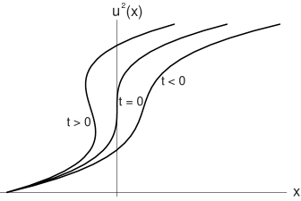
Figure 2: Formation of multi-valued solution of the mKdV equation in dispersionless limit (58). The initial data correspond to the cubic curve $x=-(u^{2}-u_{b}^{2})^{3}$ (see Eq. (60)).

For $t>0$ solution (60) becomes multi-valued function of $x$. Formation of this multi-valued region is shown in Fig. 2. For $t\geq 0$ we cannot neglect dispersion and have to consider full mKdV equation. Due to effect of dispersion the multi-valued region is replaced by the region of fast oscillations which can be represented as a modulated periodic solution of the mKdV equation (21). We rewrite this solution [see Eqs. (52), (53)] in terms of the slowly varying functions $r_{i}(x,t)$, $i=1,2,3$,

$$u(x,t)=\frac{(\sqrt{r_{3}}+\sqrt{r_{1}})(\sqrt{r_{2}}+\sqrt{r_{1}}-\sqrt{r_{3}})+(\sqrt{r_{3}}-\sqrt{r_{2}})(\sqrt{r_{1}}+\sqrt{r_{2}}+\sqrt{r_{3}}){\mathrm{sn}}^{2}(2\sqrt{r_{3}-r_{1}}\,\theta,m)}{\sqrt{r_{1}}+\sqrt{r_{3}}-(\sqrt{r_{3}}-\sqrt{r_{2}}){\mathrm{sn}}^{2}(2\sqrt{r_{3}-r_{1}}\,\theta,m)},$$ (61)

where

$$m=\frac{r_{3}-r_{2}}{r_{3}-r_{1}},\quad\theta=x+2s_{1}t=x+2(r_{1}+r_{2}+r_{3})t.$$ (62)

and functions $r_{i}(x,t)$ are governed by the Whitham equations (56). We have to find such solution of these equations that the region of oscillations matches at its end points corresponding to $m=0$ and $m=1$ to the dispersionless solution (60) which we rewrite in the form

$$x+6rt=-(r-r_{b})^{3},\quad r=u^{2},\quad r_{b}=u_{b}^{2}.$$ (63)

This means that the solution of Eqs. (56) written in implicit form

$$x-v_{i}(r)t=w_{i}(r),\quad i=1,2,3,$$ (64)

must satisfy the boundary conditions

$$\left.v_{1}\right|_{r_{2}=r_{3}}=-6r_{1},\quad\left.v_{3}\right|_{r_{2}=r_{1}}=-6r_{3};$$ (65)

$$\left.w_{1}\right|_{r_{2}=r_{3}}=-(r_{1}-r_{b})^{3},\quad\left.w_{3}\right|_{r_{2}=r_{1}}=-(r_{1}-r_{b})^{3}.$$ (66)

Then, as we shall see from the results, mean values of $u$ will match at these boundaries to the solution of dispersionless mKdV equation.

To find the solution (64) subject to the boundary conditions (65),(66), we shall follow the method developed earlier for KdV equation (see, e.g. kamch2000 ). We look for $w_{i}$ in the form similar to (56),

$$w_{i}=\left(1-\frac{L}{\partial_{i}L}\partial_{i}\right)W,\quad i=1,2,3,$$ (67)

and find that $W$ satisfies the Euler-Poisson equation

$$\partial_{ij}W-\frac{1}{2(r_{i}-r_{j})}\left(\partial_{i}W-\partial_{j}W\right)=0,\quad i\neq j.$$ (68)

For our aim it is enough to know a particular solution of this linear equation $W=\mathrm{const}/\sqrt{P(r)}$, where $P(r)$ is a polynomial with zeroes $r_{i}$ and it can be identified with polynomial (39) with taking into account Eqs. (55). The series expansion of this solution in inverse powers of $r$,

$$W=\frac{-4r^{3/2}}{\sqrt{(r-r_{1})(r-r_{2})(r-r_{3})}}=\sum_{n=0}^{\infty}\frac{W^{(n)}}{r^{n}},$$ (69)

can be considered as generating function of sequence of solutions,

$$W^{(1)}=-2s_{1},\quad W^{(2)}=2s_{2}-\tfrac{3}{2}s_{1}^{2},\quad W^{(3)}=3s_{1}s_{2}-2s_{3}-\tfrac{5}{4}s_{1}^{3},$$ (70)

where $s_{1},s_{2},s_{3}$ are the coefficients of the polynomial (39) expressed in terms of $r_{1},r_{2},r_{3}$:

$$s_{1}=r_{1}+r_{2}+r_{3},\quad s_{2}=r_{1}r_{2}+r_{1}r_{3}+r_{2}r_{3},\quad s_{3}=r_{1}r_{2}r_{3}.$$ (71)

It is easy to find that the resulting velocities

$$w_{i}^{(n)}=\left(1-\frac{L}{\partial_{i}L}\partial_{i}\right)W^{(n)},\quad i=1,2,3,$$ (72)

have the following limiting values

$$\left.w_{1}^{(1)}\right|_{r_{2}=r_{3}}\equiv\left.v_{1}\right|_{r_{2}=r_{3}}-6r_{1},\quad\left.w_{3}^{(1)}\right|_{r_{2}=r_{1}}\equiv\left.v_{3}\right|_{r_{2}=r_{1}}=-6r_{3};$$ (73)

$$\left.w_{1}^{(2)}\right|_{r_{2}=r_{3}}=-\tfrac{15}{2}r_{1}^{2},\quad\left.w_{3}^{(2)}\right|_{r_{2}=r_{1}}=-\tfrac{15}{2}r_{3}^{2};$$ (74)

$$\left.w_{1}^{(3)}\right|_{r_{2}=r_{3}}=-\tfrac{35}{4}r_{1}^{3},\quad\left.w_{3}^{(3)}\right|_{r_{2}=r_{1}}=-\tfrac{35}{4}r_{3}^{3}.$$ (75)

Thus, we see that if we take

$$w_{i}(r)=-r_{b}^{3}-\tfrac{1}{2}r_{b}^{2}w_{i}^{(1)}(r)+\tfrac{2}{5}r_{b}w_{i}^{(2)}(r)-\tfrac{4}{35}w_{i}^{(3)}(r),\quad i=1,2,3,$$ (76)

then formulae (64) satisfy all necessary conditions and define dependence of $r_{1},r_{2},r_{3}$ on $x$ and $t$ in implicit form. In Fig. 3 we have shown the dependence of $r_{1},r_{2},r_{3}$ on $x$ at $t=0.5$ and $r_{b}=5$. It is clearly seen that $r_{2}$ and $r_{1}$ coalesce at the right boundary $x_{+}$, where $m=1$, and $r_{2}$ and $r_{3}$ coalesce at the left boundary $x_{-}$, where $m=0$. Dispersionless solution is depicted by dashed line and $r_{1}$ matches this solution at $x_{-}$ and $r_{3}$ matches it at $x_{+}$.

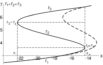
Figure 3: Dependence of the Riemann invariants $r_{1},r_{2},r_{3}$ on $x$ at some fixed value of time. The plots are calculated according to formulae (64) with $r_{b}=5$ and $t=0.5$. A dashed line represents the dispersionless solution which matches the Riemann invariants at the boundaries $x_{\pm}$ of the region of oscillations.

Let us find the laws of motion $x_{\pm}(t)$ of the boundaries of the region of oscillations. At the right boundary we have the condition

$$\left.\frac{dx}{dr_{1}}\right|_{m=1}=\left.\frac{dx}{dr_{2}}\right|_{m=1}=0,$$ (77)

which yields the expression

$$t=\tfrac{12}{35}r_{1}^{2}+\tfrac{4}{35}r_{1}r_{3}+\tfrac{3}{70}r_{3}^{2}-\tfrac{4}{5}r_{1}r_{b}-\tfrac{1}{5}r_{3}r_{b}+\tfrac{1}{2}r_{b}^{2},$$ (78)

and substitution of this expression into Eqs. (64) with $r_{1}=r_{2}$ gives the coordinate $x_{+}$ expressed in terms of the Riemann invariants $r_{1}$ and $r_{3}$:

$$x_{+}=\tfrac{1}{35}\left[-32r_{1}^{3}+2r_{3}^{3}-8r_{1}r_{3}(r_{3}-7r_{b})-8r_{1}^{2}(4r_{3}-7r_{b})-7r_{3}^{2}r_{b}-35r_{b}^{3}\right].$$ (79)

On the other hand, this value of $x_{+}$ must coincide with coordinate obtained from the dispersionless solution (63) with $t$ equal to Eq. (78),

$$x_{+}=-6r_{3}t-(r_{3}-r_{b})^{3}=\tfrac{1}{35}\left[-72r_{1}^{2}r_{3}+26r_{3}^{3}-24r_{1}r_{3}(r_{3}-7r_{b})-63r_{3}^{2}r_{b}-35r_{b}^{3}\right].$$ (80)

Comparison of these two expressions for $x_{+}$ yields the relation between $r_{1},\,r_{2}$ and $r_{3}$ at $m=1$:

$$\left(4r_{1}+3r_{3}\right)_{m=1}=7r_{b}.$$ (81)

Substitution of $r_{1}$ obtained from this equation into Eq. (78) gives

$$t=\tfrac{3}{20}(r_{3}-r_{b})^{2}.$$ (82)

Hence

$$\left.r_{3}\right|_{m=1}=r_{b}+\tfrac{2}{3}\sqrt{15t}$$ (83)

and again with the use of Eq. (81) we obtain

$$\left.r_{1}\right|_{m=1}=\left.r_{2}\right|_{m=1}=r_{b}-\tfrac{1}{2}\sqrt{15t}.$$ (84)

These formulae give values of the Riemann invariants at the right boundary as functions of time $t$. Their substitution into (79) or (80) yields the motion law of the right boundary

$$x_{+}(t)=-6r_{b}t+\tfrac{4}{3}\sqrt{\tfrac{5}{3}}\,t^{3/2}.$$ (85)

In a similar way at the left boundary $x_{-}$ the conditions

$$\left.\frac{dx}{dr_{2}}\right|_{m=0}=\left.\frac{dx}{dr_{3}}\right|_{m=0}=0$$ (86)

yield

$$t=-\tfrac{1}{30}r_{1}^{2}-\tfrac{4}{15}r_{1}r_{3}+\tfrac{4}{5}r_{3}^{2}+\tfrac{1}{3}r_{1}r_{b}-\tfrac{4}{3}r_{3}r_{b}+\tfrac{1}{2}r_{b}^{2}$$ (87)

which substitution into Eqs. (64) and (63) gives, respectively,

$$x_{-}=\tfrac{1}{5}\left[-2r_{1}^{3}-32r_{3}^{3}+8r_{1}r_{3}(4r_{3}-5r_{b})+40r_{3}^{2}r_{b}-r_{b}^{3}+r_{1}^{2}(-8r_{3}+15r_{b})\right]$$ (88)

and

$$x_{-}=\tfrac{1}{5}\left[6r_{1}^{3}+r_{1}^{2}(8r_{3}-25r_{b})-8r_{1}r_{3}(3r_{3}-5r_{b})-5r_{b}^{3}\right].$$ (89)

Their comparison yields the relation

$$\left(r_{1}+4r_{3}\right)_{m=0}=5r_{b}$$ (90)

which permits us to eliminate $r_{3}$ from Eq. (87) to obtain

$$t=\tfrac{1}{20}(r_{1}-r_{b})^{2}.$$ (91)

Hence

$$\left.r_{1}\right|_{m=0}=r_{b}-2\sqrt{3t}$$ (92)

and again with the use of Eq. (81) we obtain

$$\left.r_{2}\right|_{m=0}=\left.r_{3}\right|_{m=0}=r_{b}+\tfrac{1}{2}\sqrt{3t}.$$ (93)

Substitution of these formulae into (88) or (89) yields the motion law of the left boundary

$$x_{-}(t)=-6r_{b}t-12\sqrt{3}\,t^{3/2}.$$ (94)

The plots of $x_{+}(t)$ and $x_{-}(t)$ are depicted in Fig. 4. To the right from $x_{+}(t)$ and to the left from $x_{-}(t)$ the wave is described by the dispersionless solution (63). Between $x_{+}(t)$ and $x_{-}(t)$ we have the region of fast oscillations represented by Eq. (62) with $r_{i}(x,t)$, $i=1,2,3,$ given implicitly by Eqs. (76). The dependence of $u$ on $x$ at some fixed moment of time is shown in Fig. 5. It describes dissipationless shock wave connecting two smooth regions where we can neglect dispersion effects. At the right boundary the periodic wave tends to a sequence of separate dark soliton solutions of the mKdV equation and at the left boundary the amplitude of oscillations tends to zero.

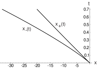
Figure 4: Dependence of coordinates $x_{\pm}$ of boundaries of the region of oscillations on time for the mKdV equation case.

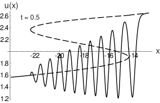
Figure 5: The dissipationless shock wave for the mKdV equation. The parameters are equal to $r_{b}=5$ and $t=0.5$. The dashed line represents the squared roots of the Riemann invariants which match the smooth solution $u(x,t)$ of the dispersionless equation at the boundaries of the region of oscillations.

III.2 Dissipationless shock wave in the KdV(2) equation (32)

The theory of dissipationless shock wave for the KdV(2) equation is similar to that for the KdV and mKdV cases. Therefore we shall present here only its main points.

The periodic solution of KdV(2) equation has the same form as in KdV equation case (see, e.g. kamch2000 ),

$$u(x,t)=r_{2}+r_{3}-r_{1}-2(r_{2}-r_{1}){\mathrm{sn}}^{2}\left(\sqrt{r_{3}-r_{1}}\,\theta,m\right),\quad m=\frac{r_{2}-r_{1}}{r_{3}-r_{1}},$$ (95)

with phase velocity

$$\theta=x-Vt,\quad V=2s_{2}-\tfrac{3}{2}s_{1}^{2},$$ (96)

corresponding to the second equation of the KdV hierarchy.

Now the periodic solution (95) is parameterized by the Riemann invariants $r_{i}$, $i=1,2,3,$ rather than by their squared roots, as it was in mKdV equation case. Hence, the solution of the dispersionless equation

$$u_{t}=\tfrac{15}{2}u^{2}u_{x}$$ (97)

near the wave breaking point should be taken in the form

$$x+\tfrac{15}{2}u^{2}=-(u-u_{b})^{3}.$$ (98)

In fact, this form is equivalent near the wave breaking point to the solution (60), since $(u^{2}-u_{b}^{2})\simeq 2u_{b}(u-u_{b})$ and the constant factor can be scaled out. Formation of multi-valued region is illustrated in Fig. 6. After taking into account the dispersion effects it should be replaced by the dissipationless shock wave.

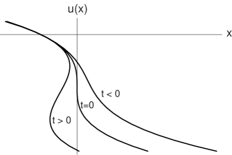
Figure 6: Formation of multi-valued solution of the KdV(2) equation in dispersionless limit (97). The initial data correspond to the cubic curve $x=-(u-u_{b})^{3}$ (see Eq. (98)).

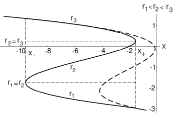
Figure 7: Dependence of the Riemann invariants $r_{1},r_{2},r_{3}$ on $x$ at some fixed value of time for the KdV(2) equation case. The plots are calculated according to formulae (99) with $u_{b}=-0.5$ and $t=0.25$. A dashed line represents the dispersionless solution which matches the Riemann invariants at the boundaries $x_{\pm}$ of the region of oscillations.

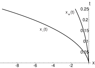
Figure 8: Dependence of coordinates $x_{\pm}$ of boundaries of the region of oscillations on time for the KdV(2) equation case.

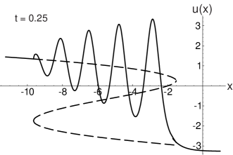
Figure 9: The dissipationless shock wave for the KdV(2) equation. The parameters are equal to $u_{b}=-0.5$ and $t=0.25$. The dashed line represents the Riemann invariants which match the smooth solution $u(x,t)$ of the dispersionless equation at the boundaries of the region of oscillations.

Within the shock wave we have modulated periodic solution (95) where $r_{i}$ are slow functions of $x$ and $t$ and their evolution is governed by the Whitham equations (56) with $V$ defined by Eq. (96). Their solution subject to the necessary boundary conditions can be found by the same method as was used in the preceding subsection. As a result we obtain

$$x-w_{i}^{(2)}t=u_{b}^{3}+\tfrac{1}{2}u_{b}^{2}w_{i}^{(1)}-\tfrac{2}{5}u_{b}w_{i}^{(2)}+\tfrac{4}{35}w_{i}^{(3)},$$ (99)

where $w_{i}^{(n)}$ are defined by formulae (70)–(72). Equations (99) define implicitly the dependence of the Riemann invariants $r_{i},$ $i=1,2,3,$ on $x$ and $t$. The resulting plots are shown in Fig. 7. At the right boundary $x_{+}$ we have soliton limit ($m=1$) and at the left boundary $x_{-}$ we have a wave with vanishing modulation.

The motion laws $x_{\pm}(t)$ can be found as in the preceding subsection, but the final formulae become now quite complicated and we shall not write them down. The corresponding plots are presented in Fig. 8. Again the region between $x_{-}(t)$ and $x_{+}(t)$ corresponds to expanding with time $t$ dissipationless shock wave. It is illustrated in Fig. 9 where the dependence $u(x)$ at fixed moment $t$ is shown. Now at one boundary bright solitons are formed and at the other boundary amplitude of oscillations tends to zero.

IV Conclusion

We have shown that GDNLS equation with finite density boundary conditions can be reduced, depending on values of the parameters $\eta$ and $\rho$, to several important continuous models—KdV, mKdV, KdV(2) and fifth-order KdV equations which describe different regimes of wave propagation in nonlinear lattice (Salerno model). The KdV(2) equation appears at such values of the parameters for which nonlinear and dispersive terms in in the KdV equation vanish, so that the main contribution in small amplitude long wave approximation is given by the third order nonlinear and fifth-order dispersion effects. This point correspond to the AL equation case, and since the AL equation is completely integrable and multi-scale method preserves complete integrability, we arrive at the second equation of the KdV hierarchy. This observation explains physical meaning of higher equations of integrable hierarchies—they give main contribution into wave dynamics if lower order effects vanish in small amplitude approximation of initial integrable equation.

The evolution equations obtained as approximations to the GDNLS equation lead in dispersionless limit for general enough initial pulses to wave breaking so that taking into account small dispersion effects leads to formation of dissipationless shock waves. We have developed the theory of these waves in framework of Whitham averaging method. Analytical expressions are obtained which describe their main characteristics—trailing and leading end points, amplitudes and wavelengths.

The phenomena described in the present paper are not restricted by the GDNL, but are characteristic features of a large class of nonlinear Schrödinger lattices, which depend on one or more free parameters.

- (1) G.B. Whitham, Linear and Nonlinear Waves, Wiley-Interscience, New York, 1974.
- (2) R.Z. Sagdeev, Collective processes and shock waves in rarified plasma, in Problems of Plasma Theory, edited by M.A. Leontovich, vol.5, (Atomizdat, Moscow, 1964).
- (3) D. Krökel, N.J. Halas, G. Giuliani and D. Grischkowsky, Phys. Rev. Lett. 60, 29 (1988).
- (4) B. L. Holian and G. K. Straub, Phys. Rev. B 18 1593 (1978); B. L. Holian, H. Flaschka, and D. W. McLaughlin, Phys. Rev. A 24 2595 (1981); D. J. Kaup, Physica 25 D 361 (1987); S. Kamvissis, Physica D 65, 242 (1993)
- (5) A.M. Kamchatnov, Nonlinear Periodic Waves and Their Modulations—An Introductory Course, World Scientific, Singapore, 2000.
- (6) M. Salerno, Phys. Rev. A 46, 6856 (1992); Phys. Lett. A 162, 381 (1992).
- (7) V.Z. Enol’skii, M. Salerno, A.C. Scott, and J.C. Eilbeck, Physica D 59, 1 (1992).
- (8) D. Hennig and G.P. Tsironis, Phys. Rep. 307, 333 (1999)
- (9) V.V. Konotop and M. Salerno, Phys. Rev. E 55, 4706 (1997).
- (10) V.V. Konotop and M. Salerno, Phys. Rev. E 56, 3611 (1997).
- (11) V.V. Konotop, Chaos, Solitons and Fractals 11, 153 (1999).
- (12) A.V. Gurevich and L.P. Pitaevskii, ZhETF, 65, 590 (1973) [Sov. Phys. JETP, 38, 291 (1973)]
- (13) V.E. Zakharov and Kuznetsov, Physica D, 18, 455 (1986)