present-time address: ]DAMTP, University of Cambridge, Wilberforce Rd., Cambridge CB3 0WA, UK.

Self-Similar Turbulent Dynamo

Abstract

The amplification of magnetic fields in a highly conducting fluid is studied numerically. During growth, the magnetic field is spatially intermittent: it does not uniformly fill the volume, but is concentrated in long thin folded structures. Contrary to a commonly held view, intermittency of the folded field does not increase indefinitely throughout the growth stage if diffusion is present. Instead, as we show, the probability-density function (PDF) of the field strength becomes self-similar. The normalized moments increase with magnetic Prandtl number in a powerlike fashion. We argue that the self-similarity is to be expected with a finite flow scale and system size. In the nonlinear saturated state, intermittency is reduced and the PDF is exponential. Parallels are noted with self-similar behavior recently observed for passive-scalar mixing and for map dynamos.

We consider the problem of magnetic-energy amplification by a homogeneous isotropic turbulence in a conducting fluid. This effect is known as the small-scale turbulent dynamo, and it is important to the dynamics of magnetic fields in astrophysical objects. It is, in fact, a generic property of random (in time and/or space) flows that they can amplify magnetic fluctuations at scales smaller than the scale of the flow itself. The amplification is a net result of stretching of the field lines by the local random strain associated with the flow Batchelor (1950); Zeldovich et al. (1984); Childress and Gilbert (1995). The fields generated by this mechanism have a characteristic structure: they concentrate in flux folds containing antiparallel field lines that reverse direction at the resistive scale and remain straight up to the flow scale Ott (1998); Schekochihin et al. (2002, 2003). It is because of the direction reversals that the magnetic energy in the wave-number space is predominantly at the resistive scale Kazantsev (1967); Kulsrud and Anderson (1992). The growing folded fields also concentrate in small parts of the system’s volume: a phenomenon called intermittency. These properties of the small-scale dynamo are most pronounced for systems where the fluid viscosity is much larger than magnetic diffusivity (magnetic Prandtl number $\text{Pr}_{\text{m}}=\nu/\eta\gg 1$), i.e., where magnetic fields reverse direction at scales much smaller than the viscous cutoff. This regime is realized in many astrophysical plasmas: examples are warm interstellar medium, intracluster and intergalactic plasmas. In this Letter, we study the volume-filling properties of the dynamo-generated fields, i.e., the distribution of the field strength.

Consider the equations of incompressible MHD:

$${d\over dt}\,{\bf u} = \nu\Delta{\bf u}-\nabla p+{\bf B}\cdot\nabla{\bf B}+{\bf f},\quad\nabla\cdot{\bf u}=0,$$ (1)

$${d\over dt}\,{\bf B} = {\bf B}\cdot\nabla{\bf u}+\eta\Delta{\bf B},$$ (2)

where $d/dt=\partial_{t}+{\bf u}\cdot\nabla$. The pressure $p$ and the magnetic field ${\bf B}$ are normalized by $\rho$ and $(4\pi\rho)^{1/2}$, respectively, where $\rho=\text{const}$ is density. Turbulence is excited by the forcing ${\bf f}$. The spatial scale of the forcing is usually much larger than the diffusion scales of the fields. In our simulations, we solve Eqs. (1–2) by a pseudospectral method. The forcing ${\bf f}$ is chosen to be random, white ($\delta$-correlated) in time, and restricted to $k/2\pi=1,2$. The code units are based on box size 1 and mean injected power $\langle{\bf u}\cdot{\bf f}\rangle=1$.

If diffusion is ignored ($\eta=0$), Eq. (2) has the following formal solution in the comoving frame:

$$\ln\left[B(t)/B_{0}\right]=\int_{0}^{t}dt^{\prime}\,{{\hat{\bf b\mkern-4.0mu}\mkern 4.0mu}{}}{{\hat{\bf b\mkern-4.0mu}\mkern 4.0mu}{}}:\nabla{\bf u}\,(t^{\prime}),$$ (3)

where ${{\hat{\bf b\mkern-4.0mu}\mkern 4.0mu}{}}={\bf B}/B$. The Central Limit Theorem suggests that $B$ should have a lognormal PDF with both the mean $\langle\ln B\rangle\propto t$ and dispersion $D\propto t$ [cf. Eq. (4)]. This implies that $\langle B^{n}\rangle\propto\exp(\gamma_{n}t)$, where the growth rates depend quadratically on the order: $\gamma_{n}\propto n(n+3)$ Zeldovich et al. (1984); Chertkov et al. (1999); Boldyrev and Schekochihin (2000). Thus, in the diffusion-free case, the intermittency of the field-strength distribution increases in time in the sense that the kurtosis $\langle B^{4}\rangle/\langle B^{2}\rangle^{2}$ and all other normalized moments $\langle B^{mn}\rangle/\langle B^{m}\rangle\langle B^{n}\rangle$ grow exponentially. In space, intermittency means that the growing fields do not uniformly fill the volume (compared to, e.g., a Gaussian field with the same energy). Assuming the equivalence of ensemble and volume averages, we may roughly interpret $\langle B^{4}\rangle/\langle B^{2}\rangle^{2}$ as an inverse volume-filling fraction.

Figure 1: Evolution of normalized moments of the magnetic-field strength. The (square root of) kurtosis of the velocity field is given for comparison. The kinematic (growth) and nonlinear (saturation) stages are demarcated in the plot.

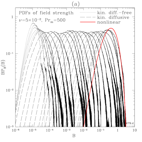
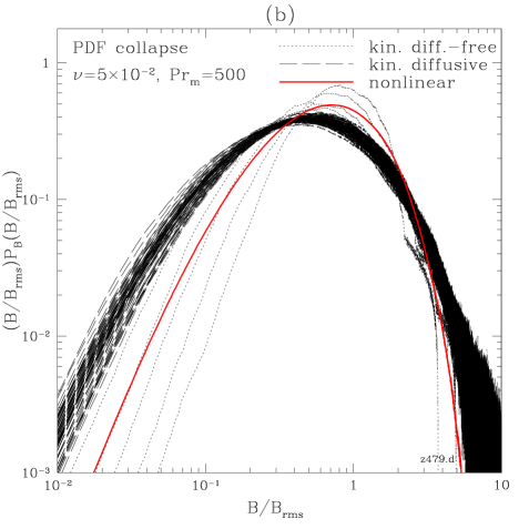
Figure 2: (a) Evolution of the PDF of the magnetic-field strength. (b) The PDFs of $B/B_{\text{rms}}$ in the kinematic regime: collapse onto a self-similar profile. The PDF in the saturated state is also shown.

In the limit of small but finite $\eta$, the small-scale dynamo can still operate, but analytical description is much harder than for the diffusion-free case. The traditional approach that makes Eq. (2) solvable in the diffusive regime is to consider a model random velocity field that is linear in space Zeldovich et al. (1984) and white in time Kazantsev (1967). The moments of $B$ can then be related to the distribution of the finite-time Lyapunov exponents associated with the velocity-gradient matrix $\nabla{\bf u}$, which is a function of time only Zeldovich et al. (1984); Chertkov et al. (1999). The result is that the growth rates of $\langle B^{n}\rangle$ still increase with $n$ as $\gamma_{n}\sim n^{2}$, i.e, intermittency continues to grow with time Chertkov et al. (1999). It has so far been an accepted view that this model adequately describes the turbulent dynamo in the large-$\text{Pr}_{\text{m}}$ limit. In fact, the picture of increasing intermittency is not borne out by numerical experiments.

In order to understand why, it is crucial to appreciate that the results obtained in the linear-velocity model apply only as long as magnetic fluctuations are “unaware” of the finiteness of the flow scale (system size). The most intuitive, albeit nonrigorous, argument as to why finite-scale effects should be important is as follows.

The fields everywhere are stretched exponentially, but with fluctuating stretching rates, so any occasional difference in field strength between different substructures tends to be amplified exponentially. Intermittency can grow with time if the system is infinite because for each moment $\langle B^{n}\rangle$, an ever smaller set of substructures can always be found in which the field has exponentially outgrown the rest of the system and which, therefore, dominantly contribute to $\langle B^{n}\rangle$. By contrast, in a finite system, only a finite number of exponentially growing substructures can exist, so the contribution to all moments must eventually come from the same fastest-growing one. The statistics of $B$ should, therefore, be self-similar, with $\langle B^{n}\rangle$ growing at rates proportional to $n$, not $n^{2}$, and all normalized moments $\langle B^{mn}\rangle/\langle B^{m}\rangle\langle B^{n}\rangle$ saturating .

This is exactly what happens in our simulations. After initial diffusion-free growth, the normalized moments saturate (Fig. 1). The PDF of the magnetic-field strength becomes self-similar: namely, the PDFs of $B/B_{\text{rms}}$ (here $B_{\text{rms}}=\langle B^{2}\rangle^{1/2}$) collapse onto a single stationary profile throughout the kinematic stage of the dynamo (Fig. 2). The large-$B$ tail of the PDF of $B/B_{\text{rms}}$ is reasonably well fitted by a lognormal distribution. Namely, suppose the PDF of $z=\ln B$ is

$$P_{z}(z)=(\pi D)^{-1/2}\exp\bigl{[}-\bigl{(}z-\langle\ln B\rangle\bigr{)}^{2}/D\bigr{]}.$$ (4)

Then $\langle B^{n}\rangle\propto\exp\left[\langle\ln B\rangle n+Dn^{2}/4\right]$, so $D=\ln\bigl{(}\langle B^{4}\rangle^{1/2}/\langle B^{2}\rangle\bigr{)}$. In the diffusive regime, $D=\text{const}$ and the field-strength statistics become self-similar: the PDF of $\zeta=\ln(B/B_{\text{rms}})$ is stationary:

$$P_{\zeta}(\zeta)=(\pi D)^{-1/2}\exp\bigl{[}-\bigl{(}\zeta+D/2\bigr{)}^{2}/D\bigr{]}.$$ (5)

The lognormal fit in Fig. 3 is obtained by calculating $D$ from the numerical data and comparing the profile (5) with the numerically calculated PDF. The fit is qualitative but decent, considering the simplicity of the chosen profile (5), large statistical errors in determining $\langle B^{4}\rangle/\langle B^{2}\rangle^{2}$ (Fig. 4), and dealiasing-induced numerical errors in resolving the field structure Schekochihin et al. (2003). The PDF at low values of $B$ appears to be powerlike (Fig. 2b), but there may be an unresolved lognormal tail at even smaller $B$. Note that the large-$B$ tail describes the straight segments of the folds, while the small-$B$ tail gives the field-strength distribution for the weak fields in the bends Schekochihin et al. (2002).

The plots in Figs. 1–3 are for a $256^{3}$ simulation of Eqs. (1–2) with $\nu=5\times 10^{-2}$ and $\text{Pr}_{\text{m}}=\nu/\eta=500$. The Reynolds number for this run is $\text{Re}=\langle u^{2}\rangle^{1/2}/\nu k_{0}\simeq 2$, (here $k_{0}=2\pi$ is the box wavenumber). Thus, the velocity field, while random, is smooth in space. This is the so-called viscosity-dominated regime, which is the only physical setting in which large $\text{Pr}_{\text{m}}$ can be resolved numerically. Interestingly, results for larger Re (“real turbulence”) and $\text{Pr}_{\text{m}}\gtrsim 1$ are very similar, especially in the kinematic regime. The reason for this is that the small-scale dynamo is always driven by the fastest eddies — the viscous-scale ones Kulsrud and Anderson (1992), — and essentially the same field-stretching mechanism applies in both synthetic one-scale dynamos Kazantsev (1967); Zeldovich et al. (1984); Childress and Gilbert (1995); Ott (1998); Schekochihin et al. (2002) and in turbulent systems with $\text{Pr}_{\text{m}}\geq 1$. In runs with $\text{Pr}_{\text{m}}=10$, $\text{Re}\simeq 100$, and even with $\text{Pr}_{\text{m}}=1$, $\text{Re}\simeq 450$ (not shown), we have found behavior analogous to that described above: saturation of normalized moments in the kinematic diffusive regime and self-similar field-strength PDFs fairly well fitted by the lognormal profile (5). In fact, the lognormal fit worked even better in these cases, which are somewhat less violently fluctuating, because velocity is not as strongly coupled to the forcing. More detailed comparisons will be reported in a future paper Schekochihin et al. (2003).

The hypothetical lognormal PDF (4) becomes self-similar only if its dispersion $D$ does not depend on time. In contrast, in the diffusion-free regime, $D\sim\gamma t$, where $\gamma\sim\nabla{\bf u}$ is the stretching rate (the turnover rate of the viscous-scale eddies). In the case of $\eta>0$ and linear velocity field, the formula for $\langle B^{n}\rangle$ derived by Chertkov et al. Chertkov et al. (1999) is also consistent with a lognormal distribution for which $D\sim\gamma t$. Both results are only valid transiently, during the time that it takes magnetic fluctuations to reach the resistive scale (in the former case) or the system (flow) scale (in the latter case). Since the scale separation is $\sim\text{Pr}_{\text{m}}^{1/2}$ and and the spreading over scales proceeds exponentially fast at the rate $\sim\gamma$ (e.g. Kulsrud and Anderson (1992)), the time during which intermittency increases is $t_{*}\sim\gamma^{-1}\ln\text{Pr}_{\text{m}}^{1/2}$. Physically, this is the time necessary to form a typical fold with length of the order of the flow scale and field reversals at the resistive scale — starting either from a flow-scale or a resistive-scale fluctuation. We might conjecture that this time determines the magnitude of the dispersion in the self-similar regime: $D\sim\gamma t_{*}\sim\ln\text{Pr}_{\text{m}}^{1/2}$, which implies that the kurtosis $\langle B^{4}\rangle/\langle B^{2}\rangle^{2}=\exp(2D)$ increases with $\text{Pr}_{\text{m}}$ in a powerlike fashion. The specific power law depends on prefactors that may be non-universal. The same holds for other normalized moments. Figure 4 is an attempt to test this hypothesis for a sequence of simulations with increasing $\text{Pr}_{\text{m}}$. The fluctuations in the kinematic regime are very large (see Fig. 1), so the error bars are too wide to allow us to claim definite confirmation of the powerlike behavior, but our results are consistent with a $\langle B^{4}\rangle/\langle B^{2}\rangle^{2}\sim\text{Pr}_{\text{m}}^{0.3}$ scaling .

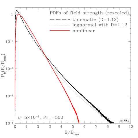
Figure 3: The PDF of $B/B_{\text{rms}}$ averaged over the kinematic diffusive stage and the lognormal profile (5) with the same $D$. Also given is the PDF in the saturated state.

We emphasize that the self-similarity reported here is statistical, not exact. Namely, it does not imply that the magnetic field is simply a growing eigenmode of the induction equation (2). Such an eigenmode does exist for some finite-scale non-random (and time-independent) flows and maps, owing essentially to the fact that the diffusion operator has a discrete spectrum in a finite domain Childress and Gilbert (1995). The self-similar PDF we have found here is a natural counterpart of this eigenmode dynamo for random flows.

Note that for the problem of passive-scalar decay, self-similar behavior was also found in certain two-dimensional maps (the so-called “strange mode” Pierrehumbert (1994); Fereday et al. (2002); Sukhatme and Pierrehumbert (2002); Thiffeault and Childress (2003)), two-dimensional non-smooth inverse-cascading turbulence Chaves et al. (2001), and even in scalar-mixing experiments Rothstein et al. (1999). In map dynamos studied by Ott et al. Du and Ott (1993); Ott (1998), moments of $B$ also grew at rates $\propto n$ (these authors related such behavior to the flux-cancellation property of the field, i.e, to the folded structure). We expect that self-similar evolution is a fundamental property of passive advection of scalar and vector fields by finite-scale flows.

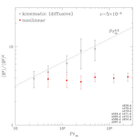
Figure 4: The kurtosis $\langle B^{4}\rangle/\langle B^{2}\rangle^{2}$ during the diffusive kinematic and the nonlinear stages of a sequence of runs with $\nu=5\times 10^{-2}$ (low Re) and $25\leq\text{Pr}_{\text{m}}\leq 2500$. All averages are over 20 time units ($\sim$ 20 turnover times).

A detailed discussion of the nonlinear saturation of the dynamo and of the magnetic-field intermittency in the saturated state is beyond the scope of this Letter. We limit ourselves to mentioning that the nonlinearity leads to a reduction of intermittency due to tighter packing of the system domain by the saturated fields (Fig. 1). It is not a surprising result: nonlinear back reaction imposes an upper bound on the field growth, and, once the strongest fields in the dominant substructure saturate, the weaker ones elsewhere have an opportunity to catch up. The PDF of the saturated field turns out to be exponential (Fig. 3, cf. Brandenburg et al. (1996); Cattaneo (1999)). Accordingly, in the nonlinear regime, the kurtosis does not depend on $\text{Pr}_{\text{m}}$ (Fig. 4). Furthermore, while $B_{\text{rms}}$ is not $\text{Pr}_{\text{m}}$-independent for finite values of $\text{Pr}_{\text{m}}$ (though $B_{\text{rms}}$ does tend to a constant value $\sim u_{\text{rms}}$ as $\text{Pr}_{\text{m}}\to\infty$), the PDF of $B/B_{\text{rms}}$ turns out to be the same for all $\text{Pr}_{\text{m}}$. Further results on the nonlinear dynamo will be reported elsewhere Schekochihin et al. (2003).