Ray chaos and ray clustering in an ocean waveguide

Abstract

We consider ray propagation in a waveguide with a designed sound-speed profile perturbed by a range-dependent perturbation caused by internal waves in deep ocean environments. The Hamiltonian formalism in terms of the action and angle variables is applied to study nonlinear ray dynamics with two sound-channel models and three perturbation models: a single-mode perturbation, a random-like sound-speed fluctuations, and a mixed perturbation. In the integrable limit without any perturbation, we derive analytical expressions for ray arrival times and timefronts at a given range, the main measurable characteristics in field experiments in the ocean. In the presence of a single-mode perturbation, ray chaos is shown to arise as a result of overlapping nonlinear ray-medium resonances. Poincaré maps, plots of variations of the action per a ray cycle length, and plots with rays escaping the channel reveal inhomogeneous structure of the underlying phase space with remarkable zones of stability where stable coherent ray clusters may be formed. We demonstrate the possibility of determining the wavelength of the perturbation mode from the arrival time distribution under conditions of ray chaos. It is surprising that coherent ray clusters, consisting of fans of rays which propagate over long ranges with close dynamical characteristics, can survive under a random-like multiplicative perturbation modelling sound-speed fluctuations caused by a wide spectrum of internal waves.

I Introduction

Low-frequency acoustic signals may propagate in the deep ocean to long ranges (up to a few thousands kilometers) due to existence of the underwater sound channel which acts as a waveguide confining the sound waves within a restricted water volume and preventing their interaction with the lossy ocean bottom Brekh . In the ray approximation, the underwater sound propagation can be modelled by a Hamiltonian system representing a nonlinear oscillator driven by a weak nonstationary external perturbation. A range-independent background sound speed profile plays the role of an unperturbed potential on which a range-dependent perturbation of the sound speed along the waveguide, that can be caused by internal waves, mesoscale eddies, ocean fronts or something else, is superimposed.

In the first papers on this topic Kras ; Pal ; Ufn , extremal sensitivity of ray trajectories to the initial conditions — ray dynamical chaos — has been found in simplified models of the waveguide. In a number of recent publications Colosi ; Sim ; AET ; Review ; Wolfs it has been realized that ray chaos should play an important role in interpretating measurements made in the long-range field experiments Duda ; Worc3250 which have been designed as a basis for ocean-acoustic tomography MunkW79 ; Akul — determining spatio-temporal variations of the hydrological characteristics on the real time scale from acoustical data. The sensitivity of chaotic rays to initial conditions and small variations of the environmental parameters causes a smearing of some timefront segments (representing time arrivals in the time-depth plane) that has been really observed in the field experiments Duda ; Worc3250 . Ray chaos seems to pose restrictions on the ray perturbation theory based applications to the tomography. On the other hand, numerical experiments Abd ; Tap ; Smir ; Viro-web ; Smir-ch show that even at long ranges there exist some stable characteristics of the sound signal which result in remarkably stable segments of the timefront — the main measurable characteristic in field experiments used to reconstruct variations in the ocean environment. In the recent paper Iomin , maxima of the distribution function of the ray travel time, which lead to clustering of rays, have been analytically found with a simplified speed profile corresponding to a quartic oscillator. It has been shown in PJTF that stable fragments of the timefront may correspond to regions of stability in the phase space. Ray stability and instability are strongly influenced by the form of the background sound speed profile.

The ray chaos studies have been especially encouraged by the field experiments Worc3250 where acoustical signals with 75 Hz center frequency and 37.5 Hz bandwidth, transmitted near the sound channel axis in the eastern North Pacific Ocean, have been recorded with a vertical receiving array between depths of 900 m and 1600 m at a range of 3250 km. The measurements have shown a clear contrast between well-resolved earlier portions of the received wavefronts, corresponding to steep rays with large values of the action variable, and smearing rear segments of the wavefronts corresponding to near-axial rays with small actions.

In this paper we study propagation of sound rays in a deep-ocean waveguide with typical sound-speed profiles under internal-wave induced single-mode, random-like, and mixed perturbations with the aim to explain and describe peculiarities of ray chaos and ray clustering that have been found in natural and numerical experiments. The paper is organized as follows. In Sec. II we give a brief description of the Hamiltonian formalism in terms of the depth-momentum and action-angle canonical variables. In Sec. III we design analytically a background sound-speed profile, modelling typical natural deep-ocean profiles. We integrate in quadratures the ray equations of motion in the range-independent environment and derive exact expressions for the angle and action variables in terms of the depth-momentum variables. Based on the designed profile, we consider two models of sound propagation. In Model 1 (Sec. III.1) we exclude from consideration the rays interacting with the ocean surface which cannot propagate over large distance because the profile parameters are chosen in such a way that practically all of them interact with lossy ocean bottom as well. Shifting the Profile 1 upwards, we obtain Model 2 with rays that may interact with the ocean surface without interacting with the bottom. In Sec. IV we derive analytical expressions for ray arrival times and timefronts at a given range with our model range-independent waveguides which should be compared with those in a range-dependent waveguide.

Section V contains results of numerical simulation with Models 1 and 2 in the presence of a single-mode perturbation induced by an internal wave. We construct Poincaré maps in the polar action-angle variables which show chains of regular islands (corresponding to different ray-medium nonlinear resonances) surrounded by a chaotic sea. A new insight into the phase-space structure is provided by plots which show by color modulation, respectively, values of variations of the action per ray cycle length and values of the range where rays interact with the bottom in terms of initial values of the action and angle variables. In the end of this section we demonstrate the possibility of determining the wavelength of the perturbation from arrival time distribution under conditions of ray chaos with our model profiles and the Munk canonical one.

In Sec. VI we study ray motion under a multiplicative noisy-like perturbation modelling sound-speed fluctuations caused by a spectrum of internal waves with flat and decreasing (with the wave number as $k^{-2}$) spectral densities. We show that some rays may form coherent clusters consisting of fans of rays propagating over long distances with close dynamic characteristics. The respective plots of variations of the action are used to clarify a mechanism of appearing coherent clusters in local zones of stability in the system’s phase space that can survive even under a noisy-like perturbation. The clusterization results in appearing prominent peaks in arrival-time distribution functions and manifests itself in timefronts of arriving signals as sharp strips on a smearing background and in plots presenting ray travel time versus starting momentum as “shelf”-like segments.

II Hamiltonian equations of ray motion in an underwater acoustic waveguide

Consider a two-dimensional underwater acoustic waveguide in the deep ocean with the sound speed $c$ being smooth function of depth $z$ and range $r$. In the geometrical-optics limit, one-way sound ray trajectories satisfy the canonical Hamilton equations LL

$$\dfrac{dz}{dr}=\dfrac{\partial H}{\partial p},\qquad\dfrac{dp}{dr}=-\frac{\partial H}{\partial z},$$ (1)

with the Hamiltonian

$$H=-\sqrt{n^{2}(z,\,r)-p^{2}},$$ (2)

where $n(z,\,r)=c_{0}/c(z,\,r)$ is the refractive index, $c_{0}$ is a reference sound speed, $p=n\sin{\phi}$ is the analog to mechanical momentum, and $\phi$ is a ray grazing angle. Only those rays that propagate at comparatively small grazing angles can survive in the ocean at long distances, the other ones attenuate rapidly interacting with the lossy ocean bottom. In the paraxial approximation, the Hamiltonian can be written in a simple form as a sum of the range-independent and range-dependent parts Ufn

$$H=H_{0}+H_{1}(r)$$ (3)

with the terms

$$H_{0}=-1+\dfrac{p^{2}}{2}+\dfrac{\Delta c(z)}{c_{0}},\quad H_{1}=\dfrac{\delta c(z,\,r)}{c_{0}},$$ (4)

where $\Delta c(z)=c(z)-c_{0}$, $\delta c(z,\,r)$ describes variations of the sound speed along the waveguide. In deriving Eqs. (4), we used the condition $|n^{2}(z,\,r)-1|\ll 1$, that is valid with natural underwater sound channels, and the approximation $n^{2}(z,\,r)-1\simeq-2\,\Delta c(z)/c_{0}$. Moreover, in the paraxial approximation the expression $p\simeq\tan{\phi}$ is valid. After making the canonical transformation from the variables $(p,\,z)$ to the action–angle variables $(I,\,\vartheta)$, the Hamiltonian may be written in the convenient form

$$H=H_{0}(I)+H_{1}(I,\,\vartheta,\,r).$$ (5)

The action variable is defined as the integral LL

$$I=\frac{1}{2\pi}\oint p\,dz=\frac{1}{\pi}\int\limits_{z_{\text{min}}}^{z_{\text{max}}}\sqrt{2\left(1+H_{0}-\frac{\Delta c(z)}{c_{0}}\right)}\,dz,$$ (6)

with $z_{\text{min}}$ and $z_{\text{max}}$ being the depths of the upper and lower ray turning points, respectively. The angle variable is defined as follows:

$$\vartheta=\dfrac{\partial G}{\partial I}=\left\{\begin{aligned} &\omega\int\limits_{z_{\text{min}}}^{z}\dfrac{dz}{p},&p>0,\\ -&\omega\int\limits_{z_{\text{min}}}^{z}\dfrac{dz}{p},&p\leq 0,\end{aligned}\right.$$ (7)

where $\omega$ is the angular frequency of spatial path oscillations, and

$$G=\int\limits_{z_{\text{min}}}^{z}p\,dz$$ (8)

is the generating function.

In a range-independent waveguide the sound-speed profile does not depend on the range $r$. In such a waveguide the Hamiltonian $H_{0}$ remains constant along the ray trajectory, and the ray equations in the action-angle variables are trivial

$$\dfrac{dI}{dr}=-\frac{\partial H_{0}}{\partial\vartheta}=0,\qquad\dfrac{d\vartheta}{dr}=\frac{\partial H_{0}}{\partial I}=\omega(I),$$ (9)

with the solution

$$I=I_{0},\quad\vartheta=\vartheta_{0}+\omega(I_{0})\,r,$$ (10)

where $I_{0}=I(r=0)$ and $\vartheta_{0}=\vartheta(r=0)$ are initial values of the action and angle, respectively. In a range-independent waveguide ray trajectories are periodic curves. In a range-dependent waveguide the Hamiltonian equations in terms of the action and angle variables take the form Ufn

$$\dfrac{dI}{dr}=-\frac{\partial H_{1}}{\partial\vartheta},\qquad\dfrac{d\vartheta}{dr}=\omega+\frac{\partial H_{1}}{\partial I}.$$ (11)

The action now does not conserve along the ray path. The equations (11) are, in general, nonintegrable and are known to have chaotic solutions even under a periodic perturbation $H_{1}$ Kras ; Pal ; Ufn ; Tap ; Dan .

III Exact solutions with model range-independent waveguides

In this section we study ray nonlinear dynamics in range-independent waveguides with model sound-speed profiles we have designed analytically. Our model profiles seem to be attractive by two reasons: they are typical in shape for natural deep-ocean background sound-speed profiles and provide analytical solutions to the ray equations including exact expressions for the action-angle variables in terms of the depth-momentum variables and analytical ones for timefronts and ray travel times. The model profile, hereafter referred as Profile 1 (or Model 1), is depicted in Fig. 1. Practically, all the rays, propagating in the corresponding waveguide, that interact with the ocean surface interact with the ocean bottom as well. Because of the strong attenuation of sound in the bottom, we will exclude such exceptional rays from consideration in numerical simulation. Shifting Profile 1 upwards to some distance, as it is shown in Fig. 2, we obtain Profile 2 (or Model 2) with rays that may interact with the ocean surface without interacting with the ocean bottom. Both the models will be considered because some characteristics of rays, propagating in the respective waveguides, may differ. The Munk canonical profile, widely used in underwater acoustics, is shown in Fig. 2b for comparison.

Figure 1: Analytic unperturbed sound-speed profile referred as Profile 1 (or Model 1).

III.1 Model 1 without reflections of rays from the ocean surface

In Ref. Dan we have introduced a background sound-speed profile, shown in Fig. 1, that models sound propagation through the deep ocean

$$c(z)=c_{0}\left[1-\dfrac{b^{2}}{2}\,(1-e^{-az})(e^{-az}-\gamma)\right],\qquad 0\leq z\leq h,$$ (12)

where $\gamma=\exp(-ah)$, $h$ is the lower border of the underwater sound channel that is the ocean bottom, $a$ and $b$ are adjusting parameters. In simulation with Model 1, we used the following values of the parameters: $a=1.0$ km^-1, $b=0.3$, $h=2.5$ km, and $c_{0}=1500$ m/s. The depth of the channel axis, where the speed of sound $c(z_{a})$ is minimal, is given by

$$z_{a}=\frac{1}{a}\,\ln{\frac{2}{1+\gamma}},$$ (13)

and the parameter $b$ is connected with $c(z_{a})$ as follows:

$$b=\dfrac{8}{1-\gamma}\,\sqrt{1-\frac{c(z_{a})}{c_{0}}}.$$ (14)

The cycle length of the ray path in the channel is given by

$$D=2\int\limits_{z_{\text{max}}}^{z_{\text{min}}}\frac{dz}{p}=\frac{2\pi}{a\sqrt{\gamma b^{2}-2E}},$$ (15)

where $E=H_{0}+1$. The Hamilton equations with the range-independent channel (12)

$$\dfrac{dz}{dr} =p,$$ (16)

$$\dfrac{dp}{dr} =-\frac{1}{2}ab^{2}e^{-az}(1+\gamma-2e^{-az})$$

can be solved exactly

$$z(r)=\dfrac{1}{a}\ln{\dfrac{a^{2}b^{2}\Bigl{[}1+\gamma-Q\cos{(\omega r+\vartheta_{0})}\Bigr{]}}{2\omega^{2}}},$$ (17)

$$p(r)=\dfrac{\omega Q\sin{(\omega r+\vartheta_{0})}}{a\Bigl{[}1+\gamma-Q\cos{(\omega r+\vartheta_{0})}\Bigr{]}},$$ (18)

where $\omega=2\pi/D$ and $\vartheta_{0}$ are the frequency and the initial phase of spatial oscillations of ray path in the channel, respectively. We used the short notation in the solutions (17) and (18)

$$Q(E)=\sqrt{(1-\gamma)^{2}+\frac{8E}{b^{2}}}.$$ (19)

The initial phase with a point source, placed at the channel axis, is

$$\vartheta_{0}=\pm\frac{\pi}{2}\mp\arcsin{\frac{Q}{1+\gamma}}.$$ (20)

The unperturbed separatrix is defined by the value $E=0$. It is a trajectory that separates propagating rays touching and not touching the bottom. Calculating the canonical variables (6) and (7) with Model 1, we find the action

$$I=\frac{b}{a}\left(\frac{1+\gamma}{2}-\sqrt{\gamma-\frac{2E}{b^{2}}}\right)$$ (21)

and the angle

$$\vartheta=\pm\frac{\pi}{2}\mp\arcsin{\frac{1+\gamma-(2\gamma-4E/b^{2})\,e^{az}}{Q}}.$$ (22)

The old canonical variables are the following functions of the new ones:

$$z(I,\,\vartheta)=\dfrac{1}{a}\ln{\dfrac{a^{2}b^{2}\,\left(1+\gamma-Q(I)\cos{\vartheta}\right)}{2\omega^{2}(I)}},$$ (23)

$$p(I,\,\vartheta)=\dfrac{\omega(I)\,Q(I)\sin{\vartheta}}{a\left(1+\gamma-Q\cos{\vartheta}\right)},$$ (24)

where

$$Q(I)=2\sqrt{\frac{(1+\gamma)\,aI}{b}-\frac{a^{2}I^{2}}{b^{2}}},$$ (25)

and the frequency of spatial oscillations is given by

$$\omega(I)=\frac{ab\,(1+\gamma)}{2}-a^{2}I.$$ (26)

The maximal (at $I=0$) and minimal (at $E=0$) values of the frequency $\omega(I)$ define the minimal and maximal ray cycle lengths, respectively

$$D_{\text{min}}=\frac{4\pi}{ab\,(1+\gamma)},\qquad D_{\text{max}}=\frac{2\pi}{ab\,\sqrt{\gamma}}.$$ (27)

The derivative $d\omega/dI$ is known as a parameter characterizing some nonlinear properties of a sound speed profile

$$\frac{d\omega}{dI}=-a^{2}.$$ (28)

The Hamiltonian can now be written as a function of the action variable only

$$H_{0}(I)=\frac{(1+\gamma)\,ab}{2}\,I+1-\frac{b^{2}(1-\gamma)^{2}}{8}-\frac{a^{2}}{2}I^{2}.$$ (29)

III.2 Normal mode amplitudes of the acoustic field in terms of ray quantities

In this section we derive an exact analytical expression for normal mode amplitudes of the acoustical wave field in the range-independent waveguide (12) in terms of ray variables whose exact solutions we have found above. The connection between ray and modal expansions of wave fields in the range-independent environment is well known Brekh . The normal modes of the unperturbed problem satisfy the wave equation

$$\frac{1}{2}\dfrac{d^{2}\psi_{m}}{dz^{2}}+k^{2}\left[E_{m}-\frac{\Delta c(z)}{c_{0}}\right]\psi_{m}=0,$$ (30)

where $k=2\pi\Omega/c_{0}$ is the wave number in the reference medium with the sound speed $c_{0}$, $\Omega$ is a carrier frequency, and $E_{m}=1+H_{0}(I_{m})$. The eigenfunctions $\psi_{m}(z)$, which represent normal modes in a range-independent waveguide, are supposed to be orthogonal and normalized. They constitute a complete set of basic functions in expanding an arbitrary wave field.

In the Wentzel–Kramers–Brillouin approximation, the eigenvalues of the action variable $I_{m}$, corresponding to the $m$-th mode, are determined by the Bohr–Sommerfeld quantization rule

$$kI_{m}=m+\frac{1}{2}.$$ (31)

The $m$-th eigenfunction $\psi_{m}(z)$ between its turning points can be represented as follows:

$$\psi_{m}(z)=\psi^{+}_{m}(z)+\psi^{-}_{m}(z),$$ (32)

where

$$\psi^{\pm}_{m}(z)=A_{m}\exp{\bigl{[}\pm i(kG_{m}(z)-\pi/4)\bigr{]}}.$$ (33)

The phase factor is given by

$$G_{m}(z)=G(z,\,I_{m})=\int\limits_{z_{\text{min}}}^{z}p_{m}(z)\,dz.$$ (34)

The $m$-th eigenvalue $p_{m}$ with the model profile (12) can be easily found from Eq. (4) to be

$$p_{m}(z)=\sqrt{2E_{m}+b^{2}(1-e^{-az})(e^{-az}-\gamma)}.$$ (35)

The integral (34) can be calculated exactly

$$G_{m}(z)=\frac{\pi I_{m}}{2}+\frac{b\,(1+\gamma)}{2a}\arcsin{\dfrac{1+\gamma-2\,e^{-az}}{Q_{m}}}+\\ +\sqrt{\gamma-\frac{2E_{m}}{b^{2}}}\arcsin{\dfrac{(1+\gamma)\,b^{2}-(2\gamma b^{2}-4E_{m})\,e^{-az}}{b^{2}Q_{m}}}-\frac{p_{m}(z)}{a},$$ (36)

where $Q_{m}=Q(I_{m})$. The amplitude of the $m$-th mode function is given by the following exact expression:

$$A_{m}(z)=\sqrt{\frac{ab\,(1+\gamma)-2a^{2}I_{m}}{4\pi p_{m}(z)}}.$$ (37)

III.3 Model 2 with rays reflecting from the ocean surface

Figure 2: Analytic unperturbed sound-speed profile referred as Profile 2 (or Model 2) and the Munk canonical profile.

By shifting Profile 1 (see Eq. (12)) upward to a distance $d$, we get Profile 2 (or Model 2) depicted in Fig. 2 as a solid curve

$$c(z)=c_{0}\left[1-\dfrac{b^{2}}{2}(1-e^{-a(z+d)})(e^{-a(z+d)}-\gamma)\right],\quad 0\leq z\leq h,$$ (38)

where $\gamma=\exp\bigl{[}-a(h+d)\bigr{]}$, $h$ is the maximal depth of the ocean, $c_{0}=c(h)$, $a$ and $b$ are adjusting parameters. In simulation with Model 2 we have used the following values of the parameters: $a=0.5$ km^-1, $b=0.6$, $h=4.0$ km, $d=0.15$ km, and $c_{0}=1535$ m/c. In contrary to Model 1, there exist in Model 2 rays which may interact with the ocean surface without interacting with the ocean bottom. We will take such rays into consideration because they can propagate to long distances in the ocean. For the surface-bounce rays $H>H_{r}$, where $H_{r}$ is given by

$$H_{r}=-1-\frac{b^{2}}{2}(1-e^{-ad})(e^{-ad}-\gamma).$$ (39)

The cycle length of a ray, reflecting from the ocean surface, is the following:

$$D_{r}=\frac{2}{a}\,\frac{\pi-\vartheta_{r}}{\sqrt{\gamma b^{2}-2E}},$$ (40)

where we used the notation

$$\vartheta_{r}=\frac{\pi}{2}-\arcsin\left[\frac{1+\gamma-(2\gamma-4E/b^{2})\,e^{ad}}{Q}\right].$$ (41)

Figure 3: The cycle length of the ray path $D$ versus the “energy” $E$ for the unperturbed Profile 2.

In Fig. 3 we show the dependence of the ray cycle length $D$ on the “energy” $E=H_{0}+1$. The respective derivative $dD/dE$ has a singularity at $E_{r}=1+H_{r}$. As in Model 1, the value $E=0$ defines the unperturbed separatrix. We were able to find exact expressions for the action

$$I=\frac{p(z=0)}{\pi a}+\frac{b}{a}\left(\frac{1+\gamma}{4}-\frac{1+\gamma}{2\pi}\arcsin{\dfrac{1+\gamma-2e^{-ad}}{Q}}-\frac{\pi-\theta_{r}}{\pi}\sqrt{\gamma-\frac{2E}{b^{2}}}\right)$$ (42)

and the angle

$$\vartheta=\left\{\begin{aligned} &\frac{\pi}{\pi-\vartheta_{r}}\left[\frac{\pi}{2}-\vartheta_{r}-\arcsin{\dfrac{1+\gamma-(2\gamma-4E/b^{2})\,e^{a(z+d)}}{Q}}\right],&p\geq 0,\\ &\frac{\pi}{\pi-\vartheta_{r}}\left[\frac{\pi}{2}+\arcsin{\dfrac{1+\gamma-(2\gamma-4E/b^{2})\,e^{a(z+d)}}{Q}}\right],&p<0,\end{aligned}\right.$$ (43)

for the surface-bounce rays. Under reflections, the ray momentum is given by

$$p(z=0)=\sqrt{2E+b^{2}(1-e^{-ad})(e^{-ad}-\gamma)}.$$ (44)

The depth-momentum canonical variables in the range $H>H_{r}$ are the following functions of the action-angle variables:

$$z(I,\,\vartheta)=\left\{\begin{aligned} &\dfrac{1}{a}\ln\dfrac{a^{2}b^{2}\left[1+\gamma+Q\cos{\left(\frac{\pi}{\pi-\vartheta_{r}}(\vartheta+\pi)\right)}\right]}{2\omega^{2}},&-\pi\leq\vartheta\leq 0,\\ &\dfrac{1}{a}\ln\dfrac{a^{2}b^{2}\left[1+\gamma-Q\cos{\left(\frac{\pi}{\pi-\vartheta_{r}}\vartheta+\vartheta_{r}\right)}\right]}{2\omega^{2}},&0\leq\vartheta\leq\pi.\end{aligned}\right.$$ (45)

$$p(I,\,\vartheta)=\left\{\begin{aligned} &\dfrac{\omega Q\sin{\left(\frac{\pi}{\pi-\vartheta_{r}}(\vartheta+\pi)\right)}}{a\left[1+\gamma+Q\cos{\left(\frac{\pi}{\pi-\vartheta_{r}}(\vartheta+\pi)\right)}\right]},&-\pi\leq\vartheta\leq 0,\\ &\dfrac{\omega Q\sin{\left(\frac{\pi}{\pi-\vartheta_{r}}\vartheta+\vartheta_{r}\right)}}{a\left[1+\gamma-Q\cos{\left(\frac{\pi}{\pi-\vartheta_{r}}\vartheta+\vartheta_{r}\right)}\right]},&0\leq\vartheta\leq\pi,\end{aligned}\right.$$ (46)

where $\omega$ is given by the same formula as in Model 1

$$\omega=a\sqrt{\gamma b^{2}-2E}.$$ (47)

As to normal modes of the unperturbed waveguide (38), they satisfy the respective wave equation (30) with the Bohr-Sommerfeld quantization rule

$$kI_{m}=\left\{\begin{aligned} &m+\frac{1}{2},\quad&H\leq H_{r},\\ &m-\frac{1}{4},\quad&H>H_{r}.\end{aligned}\right.$$ (48)

At $H\leq H_{r}$, the phase factor $G_{m}$ and the amplitude $A_{m}(z)$ of the $m$-th mode function are given by Eqs. (36) and (37), respectively. At $H>H_{r}$, we get

$$G_{m}=\frac{b}{a}\,\sqrt{\gamma-\frac{2E_{m}}{b^{2}}}\left[\arcsin{\dfrac{1+\gamma-\left(2\gamma-4E_{m}/b^{2}\right)\,e^{a(z+d)}}{Q_{m}}}+\vartheta_{r}(E_{m})-\frac{\pi}{2}\right]+\\ +\frac{(1+\gamma)\,b}{2a}\left[\arcsin{\dfrac{1+\gamma-2e^{-a(z+d)}}{Q_{m}}}-\arcsin{\dfrac{1+\gamma-2e^{-ad}}{Q_{m}}}\right]+\frac{p_{m}(z=0)-p_{m}(z)}{a}.$$ (49)

The amplitude of the $m$-th mode function at $H>H_{r}$ is

$$A_{m}(z)=\sqrt{\frac{ab(1+\gamma)-2a^{2}I_{m}}{4(\pi-\vartheta_{r})\,p_{m}(z)}}.$$ (50)

IV Ray arrival times and timefronts in range-independent and range-dependent waveguides

Internal waves in the ocean induce lateral variations of the sound speed. As a result, the ray cycle length and the ray action are not invariants as in range-independent waveguides but vary slowly along the ray path. Even very small variations of the sound speed may cause under typical conditions exponential divergence of rays with initially close grazing angles, the phenomenon known as ray chaos Ufn . The model of a “frozen” medium is usually adopted, where one may neglect temporal variations in the environment and take into account only its spatial variations due to comparatively small propagation time of sound in the ocean. Then variations of the speed of sound may be described by the expression

$$\delta c(z,\,r)=\delta c_{\text{rms}}(z)\,\xi(z,\,r),$$ (51)

where $\delta c_{\text{rms}}$ is the root-mean-square value of sound-speed fluctuations. Following to Refs. Smith1 ; Smir , we shall describe the fluctuations by the simple formula

$$\delta c_{\text{rms}}(z)=\varepsilon c_{0}\frac{z}{B}\,e^{-2z/B},$$ (52)

where $\varepsilon$ is a measure of the strength of the range-dependent perturbation and $B$, the termocline depth scale, is chosen to be 1 km. Throughout the paper, we use the perturbation models with only longitudinal modes of internal waves, i. e., $\xi(z,\,r)=\xi(r)$. Then the perturbed Hamiltonian may be written as follows:

$$H=H_{0}(I)+\varepsilon V(I,\,\vartheta)\,\xi(r).$$ (53)

Let us represent the perturbation in the form of the Fourier series over the cyclic variable $\vartheta$

$$V(I,\,\vartheta)=\frac{1}{2}\sum_{m=1}^{\infty}V_{m}(I)\,e^{im\vartheta}+\text{c.c.}.$$ (54)

The equations of motion are

$$\dfrac{dI}{dr}=-\frac{i}{2}\sum_{m=1}^{\infty}mV_{m}(I)\,e^{im\vartheta}\xi(r)+\text{c.c.},$$ (55)

$$\dfrac{d\vartheta}{dr}=\frac{2\pi}{D}+\varepsilon\frac{\partial V}{\partial I}\,\xi(r).$$ (56)

The function $V(I,\,\vartheta)$ is an analytical one with the Fourier amplitudes exponentially decreasing with increasing the number $m$. With Model 1 and perturbation (52), it has the form

$$V(I,\,\vartheta)=a^{-1-4/a}\left(\frac{4\omega^{4}(I)}{b^{4}\bigl{(}1+\gamma-Q(I)\cos{\vartheta}\bigr{)}^{2}}\right)^{1/a}\ln{\dfrac{a^{2}b^{2}\left[1+\gamma-Q(I)\cos{\vartheta}\right]}{2\omega^{2}(I)}}.$$ (57)

Methods of the acoustic tomography are actively used for studying spatio-temporal variations in the ocean on the real time scale MunkW79 ; Akul . When the sound waves propagate over long distances, an effective means for monitoring the medium is based on the effect of spatial variations of the sound speed on the signal arrival times, one of the main measurable characteristic in long-base acoustical experiments. Extensive field measurements, that have been carried out in recent years Duda ; Worc3250 , showed smearing of timefront segments in the rear of the sound pulse. Hardly resolvable microfolds in the late-arriving portions of the timefront, to be observable in field experiments, can be reasonably explained by the ray’s sensitivity to initial conditions. Without internal waves the timefront has a smooth folded accordion shape due to refraction as in Fig. 4. In the presence of internal waves, a nonuniformity of ray arrivals along the folded fronts appears (see Fig. 16). Zooming would reveal the presence of microfolds along the macroscopic segments of the timefront under consideration.

In accordance with the Fermat’s principle, ray arrival time to a point $R$ along a waveguide is calculated with the help of the Lagrangian $L$

$$t=\dfrac{1}{c_{0}}\int\limits_{0}^{R}L\,dr=\dfrac{1}{c_{0}}\int\limits_{0}^{R}(p^{2}-H)\,dr.$$ (58)

At sufficiently long ranges, $R/D\gg 1$, the Lagrangian $L$ may be considered as a function of the action

$$L(I)=2\pi\dfrac{I}{D(I)}-H_{0}(I).$$ (59)

Following to Eq. (58), ray arrival time to the point $R$ along a range-dependent waveguide is given by

$$t=\dfrac{R}{c_{0}}{\left<L(I)\right>},$$ (60)

where ${\left<\dots\right>}$ means an averaging over $r$. In a range-independent waveguide, arrival times for long-range paths can be simply calculated to be

$$t=\dfrac{RL}{c_{0}}\simeq\dfrac{R}{c_{0}}\left(2\pi\frac{I}{D}-H_{0}\right),$$ (61)

with the Lagrangian $L$ being an invariant. With a point sound source, all the invariants are functions of the initial value of the momentum $p(r=0)=p_{0}$, i. e., $t=t(p_{0})$. Ray arrival time at the fixed range $R$ is maximal with axial rays (because the sound speed is minimal at the channel axis), and decreases in average with increasing $p_{0}$. If $t(p_{0})$ is a monotonic function and a waveguide is range-independent, the so-called timefront, which represent ray arrivals in time-depth plane, can be calculated explicitly from the equation for the trajectory (see, for example, Eq. (23) for Model 1) with the parameters being functions of the Lagrangian $L$.

In order to demonstrate it in Model 1 with the range-independent waveguide shown in Fig. 1, we use Eq. (59) to find the action

$$I(L)=\frac{1}{a}\sqrt{2+\frac{b^{2}(1-\gamma)^{2}}{4}-2L},$$ (62)

the spatial frequency of nonlinear oscillations

$$\omega(L)=a\left(b\,\frac{1+\gamma}{2}-aI(L)\right),$$ (63)

and the quantity

$$Q(L)=2\sqrt{\frac{(1+\gamma)\,aI(L)}{b}-\frac{a^{2}I^{2}(L)}{b^{2}}},$$ (64)

as functions of the Lagrangian $L$. After substituting Eqs. (60), (62)–(64) into the ray-trajectory equation (23), we get the timefront of the sound signal in the waveguide with the sound-speed Profile 1

$$z(t)\simeq\dfrac{1}{a}\ln{\dfrac{a^{2}b^{2}\Bigl{[}1+\gamma-Q(t)\cos{\bigr{(}\omega(t)R+\vartheta_{0}\bigr{)}}\Bigr{]}}{2\omega^{2}(t)}}.$$ (65)

The respective plot, presenting ray depths against arrival times at the range $R=1000$ km, is shown in Fig. 4. We see a typical two-folded accordion-like structure due to refraction with positive and negative values of grazing angle. The ray arrivals are spread in a smooth and predictable way with the late-arriving portion of the timefront formed by the axial rays.

Figure 4: Timefront for the unperturbed Profile 1: ray depth $z$ versus ray travel time $t$ at the range 1000 km.

In the presence of a perturbation, timefront can be computed approximately as a sum of representing points of sound pulses

$$T(z,\,t)\simeq\sum_{i}T_{i}=\sum_{i}\delta(z-z_{i})\,\delta(t-t_{i}),$$ (66)

where $z_{i}$ and $t_{i}$ are the depth and arrival time of the $i$-th pulse. With the help of Eq. (23), the depth for each pulse $z$ may be written as a function of initial $I_{0}$, final $I_{f}$, and mean, ${\left<I\right>}$, values of the action, which may be considered as independent variables under conditions of strong chaos

$$z\simeq\dfrac{1}{a}\ln{\dfrac{a^{2}b^{2}\Bigl{[}1+\gamma-Q(I_{f})\cos{\bigl{(}\omega({\left<I\right>})R+\vartheta_{0}(I_{0})\bigr{)}}\Bigr{]}}{2\omega^{2}(I_{f})}}.$$ (67)

Let us consider now distribution of rays over their arrival times, $f(t,\,R)$, at a fixed range $R$. In a range-independent waveguide, it is determined by an initial distribution of grazing angles only. The respective distribution function for rays, started at small grazing angles with $\phi_{0}\simeq p_{0}$ (that may propagate over large distances), is $f_{0}(p_{0})$. Using the condition of the conserved normalization

$$\int f_{0}(t,\,R)\,dt=\int f_{0}(p_{0})\,dp_{0},$$ (68)

we get

$$f_{0}(t,\,R)=f_{0}(p_{0})\dfrac{dp_{0}}{dt}.$$ (69)

With Model 1 we get from Eqs. (61), (4), (15) and (21)

$$f_{0}(t,\,R)=\frac{f_{0}(p_{0})c_{0}\bigl{[}b\,(1+\gamma)-2U(t)\bigr{]}}{RU\sqrt{b\,(1+\gamma)U(t)-U^{2}(t)}},$$ (70)

where the short notation is used

$$U(t)=\sqrt{\frac{b^{2}}{4}\left(1-\gamma\right)^{2}+2-\frac{2c_{0}t}{R}}.$$ (71)

In a range-dependent waveguide, the distribution function of ray arrival times is given by

$$f(t,\,R)=AF(t,\,R)\,f_{0}(p_{0})\dfrac{dp_{0}(t)}{dt},$$ (72)

where $A$ is a normalization constant. The function $F(t,\,R)$ describes the effect of the range dependence of the sound speed on the distribution of ray arrival times. It is defined, mainly, by the structure of the phase space of the perturbed system PJTF . We shall use the function $F(t,\,R)$ as a convenient tool for analyzing clusterization of rays.

It should be noted that the formulas for arrival times (61) and timefronts (65) and (67) are approximated ones. Comparing Fig. 4, plotted using (65), with numerical simulation shown in Fig. 12a, one can see the difference between the two timefronts especially in the neighbourhoods of extrema. However, these formulas provide a correct general image of timefronts and give a simple analytical connection between measurable ray characterictics and the phase-space ray variables which can be used to explain such peculiarities of timefronts as sharp stripes.

V Ray chaos in the presence of a single-mode perturbation

V.1 The phase-space structure

In this section we consider a single-mode sound-speed perturbation (51) with $\delta c_{\text{rms}}(z)$ given by (52) and the horizontal dependence of the internal-wave induced perturbation given by

$$\xi(r)=\cos{kr}=\cos{\frac{2\pi r}{\lambda}},$$ (73)

where $\lambda$ is the wavelength of the internal wave. The Hamilton equations take the form

$$\dfrac{dI}{dr}=-\frac{i}{2}\varepsilon\sum_{l,\,m}lV_{lm}e^{im\Psi}+\text{c.c.},$$ (74)

$$\dfrac{d\vartheta}{dr}=\omega+\frac{\varepsilon}{2}\sum_{l,\,m}\frac{V_{lm}}{dI}\,e^{im\Psi}+\text{c.c.},$$ (75)

where the new phase $\Psi=\vartheta-\dfrac{lkr}{m}+\dfrac{\phi_{0}}{m}$ is introduced. Ray trajectories are captured in a ray-medium space nonlinear resonance if the condition

$$m\omega(I)=lk,$$ (76)

is satisfied with $l$ and $m$ being integers. This condition can be satisfied at different values of the action variable $I_{\text{res}}$ corresponding to resonant tori. Phase oscillations in vicinities of the resonant tori are described by the universal Hamiltonian of nonlinear resonance Ufn ; Chir

$$H_{u}=m\left(\frac{1}{2}\,\bigl{|}\omega^{\prime}_{I}(I_{\text{res}})\bigr{|}\left(\Delta I\right)^{2}+\varepsilon|V_{lm}|\cos{m\Psi}\right),$$ (77)

where $\omega^{\prime}_{I}(I_{\text{res}})=d\omega(I_{\text{res}})/dI$. The width of the resonance in terms of spatial frequency can be approximately estimated as

$$\Delta\omega=|\omega^{\prime}_{I}|\Delta I=2\sqrt{\varepsilon|\omega^{\prime}_{I}|V_{lm}},$$ (78)

where $\Delta I$ is the width of the nonlinear resonance in terms of the action variable. In accordance with Chirikov’s criterion Chir , global chaos may arise if

$$\frac{\Delta\omega}{\delta\omega}\simeq 1,$$ (79)

i. e., if two nonlinear resonances, centered at $\omega$ and $\omega+\delta\omega$, overlap. Those resonances that overlap slightly form islands in the phase space, areas of stable ray motion in a chaotic sea. Nearby the island’s borders, one can find the so-called zones of stickiness where chaotic trajectories may be localized for long distances $r$ Zchaos .

To visualize the structure of the phase space, we construct a Poincaré map integrating numerically the ray equations for Model 1 with the single-mode perturbation (73). Figure 5 demonstrates such a map with the perturbation wavelength $\lambda=10$ km and a comparatively weak perturbation strength $\varepsilon=0.0025$. It is a two-dimensional slice of the ray motion in a three-dimensional space $(I_{x},\,I_{y},\,r\mod\lambda)$ with $I_{x}=I\cos\vartheta$ and $I_{y}=I\sin\vartheta$ being the polar action-angle variables normalized to the separatrix value of the action $I_{s}$ (given by Eq.(21) at $E=0$) which is a maximal acceptable value of the action.

A typical (with Hamiltonian systems) picture with stable islands filled with regular trajectories surrounded by a chaotic sea is seen in the figure. The chains with 5 and 6 islands correspond to the primary resonances of the first order ($l=1$) with $m=5$ and 6, respectively. The chain with 11 islands is located between them and corresponds to the second-order resonance with $l=2$ and $m=11$. Even a higher-order resonance with 16 islands (between the $(l=1,\ m=5)$ and $(l=2,\ m=11)$ resonances) is seen in Fig. 5. Concentration of points near island’s boundaries indicates sticky trajectories.

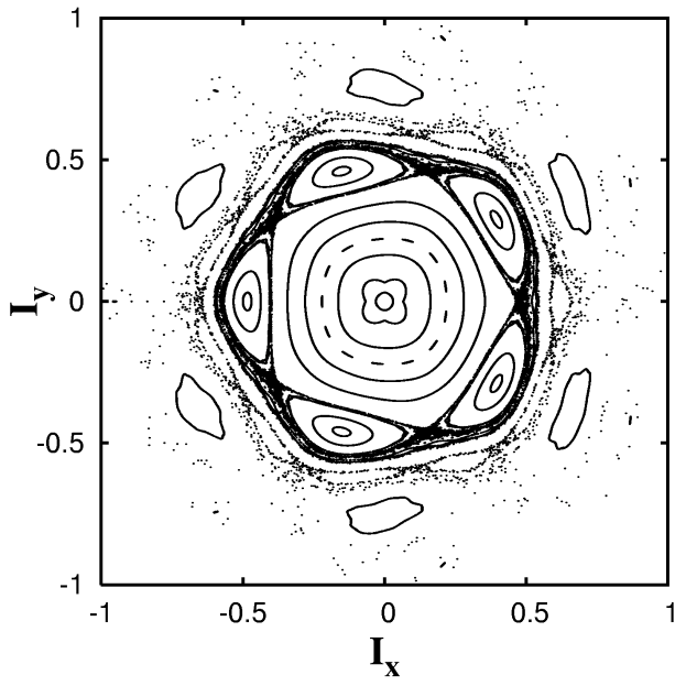
Figure 5: Poincaré map in the normalized polar action–angle variables for Model 1 with the parameters of the periodic perturbation, $\lambda=10$ km and $\epsilon=0.0025$.

Figure 6 shows the Poincaré map with rays that may reflect from the ocean surface (Model 2 with $\varepsilon=0.005$ and $\lambda=10$ km). In difference from Model 1, a stochastic layer appears inside the separatrix loop in a vicinity of the critical value of the action $I_{r}=I(H_{r})$ (Fig. 6a). We remind that reflection of rays from the ocean surface in Model 2 occurs at $H>H_{r}$ (see Eq. (39)). The origin of the localized stochastic layer can be explained as follows. The distance between the resonances of the $m$-th and $m+1$-th orders in terms of spatial frequency is equal to

$$\delta\omega=\frac{k}{m}-\frac{k}{m+1}\simeq\frac{\omega^{2}}{k}\propto D^{-2},$$ (80)

and decreases rapidly with increasing $D$. Since the ray cycle length $D$ has a local maximum at $E=E_{r}$ (Fig. 3), the resonance overlapping in accordance with (79) is maximal near $I(E_{r})$. This stochastic layer is isolated from the separatrix by invariant curves. As a result, the respective rays are trapped inside the layer forever and their motion is strongly influenced by the fractal microstructure of the stochastic layer Zas-fr ; Zchaos ; Zas-PhA . The fine structure of the phase space is demonstrated in Fig. 6b where a zoom of the region of the stochastic layer near $\vartheta=0$ is shown. Chains of microislands corresponding to primary and secondary resonances are seen in the figure. It should be noted that an analogous localized stochastic layer has been found with the Munk canonical profile Smir ; Zas-fr .

a)

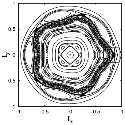
b)

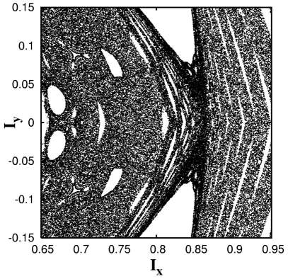
Figure 6: (a) Poincaré map in the polar normalized action–angle variables for Model 2 with the parameters of the periodic perturbation, $\lambda=10$ km and $\epsilon=0.005$. (b) Zoom of the small region of the stochastic layer indicated in (a).

Another way to visualize the phase-space structure is provided by the plot that shows by color modulation values of variations of the action during the ray cycle length $\Delta I$ in the plane of initial values of the action and angle variables normalized to the separatrix value $I_{s}$ and $\pi$, respectively. More exactly, $\Delta I$ is a variation of the action between to successive crossings of the line $\theta={\rm const}$ by a ray. It depends on the initial value of the range $r_{0}$ and may strongly vary in the chaotic regime. It is a distribution of variations of the action over the phase space that has important physical meaning. The number of positive variations of the action (“hills”) and the number of its negative variations (“hollows”) are stable characteristics of the system (independent on initial conditions) describing the phase oscillations. The respective map for Model 1 with a single-mode perturbation, presented in Fig. 7, demonstrates an alternating “hills” and “hollows” corresponding to different values of the phase $\Psi$. Due to the phase dependence, this structure periodically depends on initial values of the range variable $r$. The “hills” and “hollows” are separated from each other by “zero lines”, which correspond to zero variations of the action per cycle length, and may be “stable” and “unstable”. The “stable” ones transverse the elliptic points of the potential in Eq. (77), and the “unstable” ones transverse the respective hyperbolic points. It should be noted that “hills” and “hollows” may intersect each other.

Spatial variations of the sound speed along a waveguide may cause the known effect of ray escaping Kras when some rays reach the unperturbed separatrix due to diffusion in the action and quit the sound channel. Those rays are supposed to quit the channel which interact with the ocean bottom and therefore attenuate rapidly. First of all, steep rays with comparatively small arrival times (corresponding to higher modes of the sound field) will escape. The escaping takes place even under an adiabatic perturbation Krav but it has peculiarities under the ray chaos conditions.

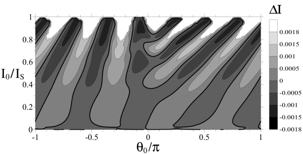
Figure 7: Plot representing variations of the action $\Delta I$ per ray cycle length for Model 1 ($\lambda=10$ km and $\epsilon=0.005$) in the plane of the normalized initial values of the action and angle. Bold lines correspond to zero variations of the action per ray cycle length.

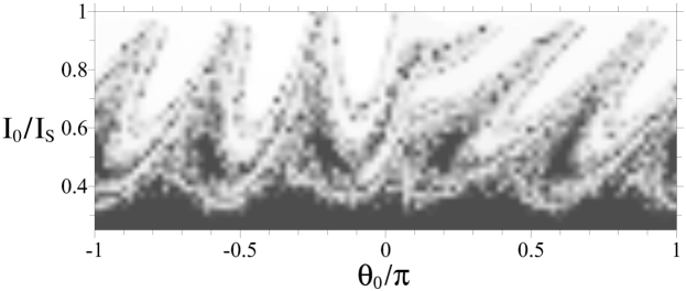
Figure 8: Plot representing the values of the range $r$, where rays interact with the ocean bottom, for the same model and the same parameters as in Fig. 7. White color corresponds to those rays that quit the channel during the first ray cycle, i. e. at $r\leq 70$ km.

In the plot, presented for Model 1 in Fig. 8, color modulates the values of the range $r$ where rays interact with the ocean bottom, with white color corresponding to rays which quit the waveguide during the first cycle, i. e. at $r\leq 70$ km (which is a cycle length of a trajectory nearby the separatrix) whereas the black one corresponds to the values $r\geq 1000$ km. As in the case with variation of the action, distribution of the values of range for the rays interacting with the ocean bottom is a stable characteristic of the system. Topology of the plot is complicated in those areas in the $\left(I_{0}/I_{s}\right)$ — $\left(\vartheta_{0}/\pi\right)$ plane which correspond to the stochastic layer. Its patchiness reflects a complicated inhomogeneity of the phase space. We want to stress that channels for escaping are formed in the same places where the “hills” are situated in the plot representing variations of the action per ray cycle length (Fig. 7). The values of the action variable grow rapidly in such channels resulting in increasing trajectory amplitudes. One can see in Fig. 8 black spots corresponding to those ranges of the initial conditions of ray trajectories that never quit the waveguide. They correspond to the respective islands of regular motion on the Poincaré map (Fig. 5). The patched dark areas between the channels with rapidly escaping rays correspond to the initial conditions with long but finite lengths of escaping. The angular structure of the distribution of the lengths of escaping in the phase space is an evidence of a non-ergodic ray diffusion. In difference from the plot representing variations of the action per ray cycle length, the plot with escaping rays has a manifested patched structure due to fractal properties of the phase space typical for open chaotic Hamiltonian systems with weak mixing (for a review see Zas-PhA ). The hierarchy of islands and chains of islands with sticky zones near the island’s boundaries, which are repeated at all scales of resolution, produces dynamical traps where representing particles may be trapped for a long distance (time). It results eventually in anomalous diffusion and power-law distribution functions Zas-PhA . It is worthwhile to mention that escaping of rays is an analog of trapping (escaping) of chaotically advected passive particles in open hydrodynamic flows (see, for example, Dan2 ).

V.2 Timefront structure under a periodic perturbation

Let us consider now the role of the ray-medium nonlinear resonance in forming the structure of timefronts of sound signals. Due to nonlinear resonance, the ray arrival time of a sound signal along a given ray, captured in a nonlinear resonance near the given value of the action $I_{\text{res}}$, tends to its unperturbed value $t(L_{\text{res}})$ with increasing the distance Ufn

$$t(L_{\text{res}})=\frac{RL(I_{\text{res}})}{c_{0}}.$$ (81)

If the width of the resonance is sufficiently large and if there are sufficiently many rays captured in the resonance, the distribution function $F(t,\,R)$ (see Eq. (72)) has a pronounced peak near the value $t(L_{\text{res}})$. Moreover, it is possible with the help of $F(t,\,R)$ to find the spatial period of a perturbation mode if the arrival time is unambiguously defined by the ray cycle length PJTF . Inverting the resonance condition (76), we get

$$lD_{\text{res}}=m\lambda.$$ (82)

There can be several peaks of the function $F(t,\,R)$ with large amplitudes corresponding to resonances with small $m$ at $l=1$. Thus, if $F(t,\,R)$ exhibits at least two distinct peaks with comparable amplitudes, we can determine the period of a single-mode perturbation as

$$\lambda=D(t_{\text{res1}})-D(t_{\text{res2}}),$$ (83)

where $t_{\text{res1}}$ and $t_{\text{res2}}$ are arrival times corresponding to the two peaks. In general, the values of $D(t_{\text{res}})$ can be calculated numerically with the help of Eq. (61). Our model Profiles 1 and 2 admit analytical calculation of the resonant cycle length. In Model 1, for example, one can deduce from Eq. (61) a formula connecting the ray cycle length $D$ with the arrival time $t$

$$D(t)=\frac{2\pi}{a}\left(b\,\frac{1+\gamma}{2}-\sqrt{\frac{b^{2}}{4}\left(1-\gamma\right)^{2}+2-\frac{2c_{0}t}{R}}\right)^{-1}.$$ (84)

The upper panel in Fig. 9 shows the function $F(t,\,R)$ corresponding to the timefront computed at $R=1000$  km with Profile 1, the perturbation wavelength $\lambda=10$ km, the perturbation strength $\varepsilon=0.0025$ and the other parameters to be specified in the preceding section. Results at the range $R=1000$  km are represented in this figure by solid lines with the lower axis showing the respective values of travel times. Local concentrations of points in the respective timefront (not shown), correspond to two sharp peaks of the function $F(t,\,R)$ at $t_{\text{res1}}\simeq 671.84$ s and $t_{\text{res2}}\simeq 672.54$ s, with the left one corresponding to the resonance $(l=1,\ m=6)$ and the right one belonging to the resonance $(l=1,\ m=5)$. Using the formula (84), one can estimate the respective resonant cycle lengths, $D(t_{\text{res1}})\simeq 60.6$ km and $D(t_{\text{res2}})\simeq 50.0$ km, and find numerically the perturbation wavelength, $\lambda_{\text{cal}}\simeq 10.6$ km. Note that the upper panel in Fig. 9 demonstrates an additional smaller peak at $t\simeq 672.25$ s corresponding to the second-order resonance with $l=2$ and $m=11$ that is manifested on the Poincaré map in Fig. 5 as a chain of islands between the first-order resonant islands. It has a comparatively small amplitude because the width of this high-order resonance and the frequency of phase oscillations are comparatively small. The satellite peak of the primary resonance $(l=1,\ m=6)$ seems to be formed by chaotic rays sticking for a long distance to respective resonant islands but quitting this zone somewhere. Note that this peak was absent when we have computed the distribution function of ray arrival times at $R=3000$ km.

The upper panel in Fig. 10 shows the function $F(t,\,R)$ with Model 1 at the increased value of the perturbation amplitude $\varepsilon=0.005$ for which ray chaos is stronger. Because of a large overlapping of the nonlinear resonances, the peak corresponding to the resonance with $l=1$ and $m=6$ has a smaller amplitude than the respective peak in Fig. 9 and disappears at $R=3000$ km at all. The peak, corresponding to the higher-order resonance with $l=2$ and $m=11$ is absent in Fig. 10. The upper panel in Fig. 11 shows the function $F(t,\,R)$ with Model 2 at $\varepsilon=0.005$. The left peak corresponds to the resonance ($l=1$, $m=5$) which is seen on the Poincaré map in Fig. 6 whereas the right peak corresponds to the stochastic layer near $I(H_{r})$. Since diffusion inside this layer is localized the respective rays have close arrival times and form a cluster.

Figure 9: Normalized function of distribution of ray arrival times for Model 1 with the periodic perturbation ($\lambda=10$ km and $\varepsilon=0.0025$) and an imposed multiplicative noise with different values of its strength $\alpha$. The solid lines represent results at the range 1000 km (see the lower axis for travel times), while the dashed lines are computed at the range 3000  km (see the upper axis for travel times). The upper panel shows the function with a purely periodic perturbation.

Figure 10: The same as in Fig. 9 but with the parameters of the periodic perturbation, $\lambda=10$ km and $\varepsilon=0.005$.

Figure 11: The same as in Fig. 10 but for Model 2.

In order to demonstrate the possibility of determining the wavelength of an internal wave from the ray arrival time distribution under conditions of ray chaos not only with our model background profiles, we have computed the timefront and the respective function $F(t,\,R)$ with the Munk canonical background profile (Fig. 2) with a periodic perturbation Smith1 ; Zas-fr ; Wierc

$$c(z,\,r)=c_{0}\left[1+\mu\,(\eta-1+e^{-\eta})+\varepsilon\frac{z}{B}\,e^{-2z/B}\cos{\frac{2\pi r}{\lambda}}\right],$$ (85)

where $c_{0}=1500$ m/s, $\mu=0.0057$, $\eta=2(z-z_{a})/B$ is a normalized depth, and $B=1$ km. The depth of the channel axis is chosen to be $z_{a}=1$ km, $\varepsilon=0.005$ and $\lambda=5$ km. The results, shown in Fig. 12 at the range $R=2000$ km, reveal two distinct peaks of the function $F(t,\,R)$, the left one at $t_{\text{res1}}\simeq 1329.9$ s corresponds to $D(t_{\text{res1}})\simeq 55$ km and the right one at $t_{\text{res2}}\simeq 1331.8$ s corresponds to $D(t_{\text{res2}})\simeq 50$ km giving the difference to be equal to the perturbation wavelength $\lambda=5$ km. The resonant cycle lengths with the Munk profile have been found numerically with the help of Eq. (61).

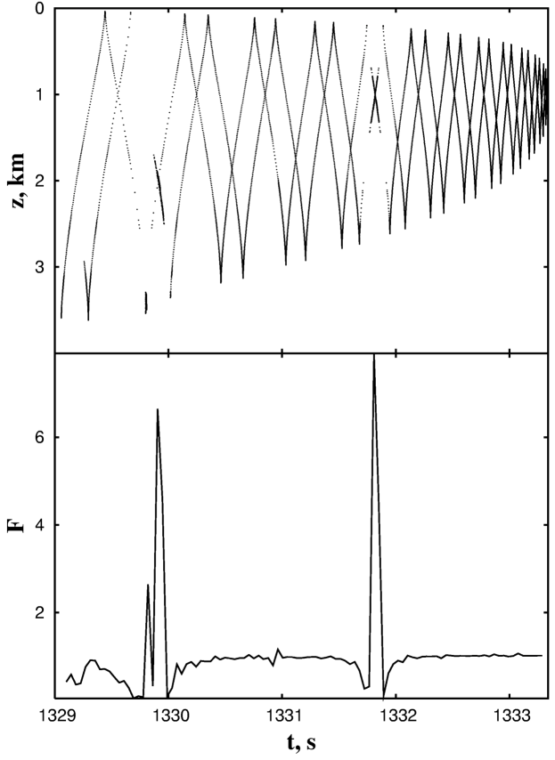
Figure 12: Timefront and the corresponding function of distribution of ray arrival times for the Munk canonical profile with the parameters of the periodic perturbation, $\lambda=5$ km and $\varepsilon=0.005$.

Generally speaking, determining perturbation wavelength is not always possible even in the case of a single-mode perturbation. It is necessary to have at least two chains of slightly overlapped primary resonances with $l=1$, and sufficiently large number of rays should be captured in these resonances.

Due to stable motion of rays, captured in a nonlinear resonance, their initial and final values of the action are in a comparatively narrow interval $\delta I$ approximately proportional to the resonance width $\Delta I$. In accordance with Eq. (67), depths of arrivals of the resonant rays at a given range $R$ are distributed over narrow intervals. In such a way, double sharp strips (see Fig. 12a), corresponding to ray clusters with positive and negative launch angles, appear in the respective timefronts.

VI Ray motion in the presence of a multiplicative noise

VI.1 Ray equations with noise

Internal waves in the deep ocean are known to have a broadened continuous spectrum of horizontal wavenumbers $k$ which may be adequately described by the empirical Garrett–Munk spectrum GM1 with the spectral energy density decreasing with increasing $k$. The periodic internal-wave induced perturbation of the sound speed to be considered in the preceding section is a useful but not realistic approximation. From the theoretical point of view, the sound-speed perturbations due to internal waves should be considered as a random function with given statistical characteristics. Under a noisy-like perturbation, there are no specified resonances in ray dynamics which, however, is strongly influenced by the presence of a nonlinear sound-speed profile Beron-Vera .

Let $\xi(r)$ be a stationary stochastic perturbation representing the sound-speed fluctuations caused by internal waves which is defined as a spectral decomposition

$$\xi(r)=\int\limits_{-\infty}^{\infty}S(k)e^{-ikr}dk,$$ (86)

where $S(k)=S_{0}(k)\,e^{-i\phi(k)}$ and $\phi(k)$ is a random function of the wave number $k$ distributed equally over the interval $[0:2\pi]$. The perturbation is assumed to be a Gaussian process with normalized first and second moments

$${\left<\xi(r)\right>}=0,\quad{\left<\xi^{2}(r)\right>}=\frac{1}{2}.$$ (87)

We assume that the horizontal scale of the internal-wave induced fluctuations is much less than the scale of the range variations of the action, and the diffusion approximation can be adopted. The perturbation amplitude depends on the angle variable $\vartheta$ and is maximal near the upper turning point, $\vartheta=0$. So, the ray cycle length $D$ gives us a characteristic scale of the range variations of the action. In simulation, we realize the process $\xi(r)$ as a sum of a large number $(\geq 1000)$ of harmonics distributed in the range $k\in[2\pi/100:2\pi/1]$ km^-1. Two spectral models of the sound-speed fluctuations, $S_{0}(k)=\text{const}$ and $S_{0}(k)\propto k^{-2}$, have been used.

The Hamilton equations of motion

$$\dfrac{dI}{dr}=-\varepsilon\,\frac{\partial V}{\partial\vartheta}\,\xi(r),\quad\dfrac{d\vartheta}{dr}=\omega(I)+\varepsilon\,\frac{\partial V}{\partial I}\,\xi(r)$$ (88)

provide the description of sound-ray trajectories through the deep ocean with a broad spectrum of internal waves inducing the respective spectrum of the sound-speed fluctuations. Substituting the Fourier decomposition (54) in the first equation (88) and taking into account that $\vartheta=\omega(r)r+\vartheta_{0}$, we can write down the variation of the action over the period as

$$\Delta I=\varepsilon\sum_{m=1}^{\infty}mV_{m}(I)\Omega_{m},$$ (89)

$$\Omega_{m}=-\frac{ie^{im\vartheta_{0}}}{2}\int\limits_{0}^{\infty}\int\limits_{0}^{D}S(k)e^{i(m\omega-k)r}dk\,dr+\text{c.c.}$$ (90)

In order to find $\omega(r)$ let us rewrite the second equation (88) as

$$\omega(r)-\omega(I_{0})=\varepsilon\frac{dV}{dI}\,\xi(r),$$ (91)

where $I_{0}$ is the initial value of the action. Assuming the correlation length of the random process $\xi(r)$ to be small as compared with the ray cycle length, $r_{\xi}\ll D$, we introduce the “fast” variable $x=r/r_{\xi}$ which is connected with the angle variable as follows:

$$x=\frac{\vartheta-\vartheta_{0}}{\omega r_{\xi}}.$$ (92)

The variable $\omega(x)$ is now treated as a function of $x$ and modelled as a Markovian process with independent increments characterized by the normal distribution

$$\upsilon\left[w(x),\,I_{0}\right]=\frac{1}{\sqrt{2\pi}\sigma}\exp\left(-\dfrac{\left(\omega-\omega(I_{0})\vphantom{\bigl{(}}\right)^{2}}{2\sigma^{2}}\right),$$ (93)

with the variance depending on $x$ and $\vartheta_{0}$

$$\sigma^{2}(x,\,\vartheta_{0})=\frac{\varepsilon^{2}}{2}\int\limits_{0}^{x}\left(\frac{dV(x^{\prime},\,\vartheta_{0})}{dI}\right)^{2}\,dx^{\prime}.$$ (94)

The main contribution to the integral (90) provides the points of a stationary phase given by the wavenumbers $k_{m}=m\omega(x)$. So we get

$$\Omega_{m}=\pi{\left<S_{m}[k_{m}(x)]\cos[m\vartheta_{0}-\phi[k_{m}(x)]]\right>}_{k_{m}(x)}=\pi\int S_{m}[k_{m}(x)]\cos[m\vartheta_{0}-\phi[k_{m}(x)]]\rho(k_{m})\,dk_{m},$$ (95)

where $\rho(k_{m})$ is the respective probability density. Because the perturbation $V(\vartheta)$ and its derivative $dV/dI(\vartheta)$ have a sharp maximum in a neighbourhood of $\vartheta=0$ and are approximately zero outside, we can assume $\rho(k_{m})\simeq\upsilon(k_{m})$ at $\sigma=\sigma(x=-\vartheta_{0}/\omega r_{\xi})$. The integral (90) is now given by

$$\Omega_{m}=\pi S_{m}^{\text{eff}}\cos{(m\vartheta_{0}-\phi_{m}^{\text{eff}})},$$ (96)

where $\phi_{m}^{\text{eff}}$ and $S_{m}^{\text{eff}}$ are an effective phase and amplitude, respectively. The amplitude is

$$S_{m}^{\text{eff}}=\int\limits_{0}^{\infty}S_{0}(k_{m})\,\rho(k_{m})\,dk_{m},$$ (97)

where $k_{m}=m\omega$. As a result, we find the variation of the action over the ray period

$$\Delta I=\varepsilon\pi\sum_{m=1}^{\infty}mV_{m}(I)S_{m}^{\text{eff}}\cos{(m\vartheta_{0}-\phi_{m}^{\text{eff}})},$$ (98)

as a sum of “resonant” terms.

As in the case with a single-mode perturbation, we compute plots which show by color modulation values of variations of the action per a ray cycle length, $\Delta I$, in the plane of the normalized initial values of the action and angle variables. The plot in Fig. 13 is computed with Model 2 and the flat spectrum $S_{0}(k)=\text{const}$ ($\varepsilon=0.005$). To visualize the borders between positive (“hills”) and negative (“hollows”) values of $\Delta I$, the lines with $\Delta I=0$ are bolded in Fig. 13. In the range of comparatively small values of the action, the first Fourier harmonic $V_{1}$ in the expansion (98) is expected to be dominant. Really, only one “hill” is present in the figure in the range $0<I_{0}/I_{s}<0.2$. With increasing the action values, the higher-order terms in (98) begin to play a more significant role, and the number of “hills” is expected to rise in the respective ranges on the plot representing variations of the action per ray cycle length. In Fig. 13 we see two “hills” in the range $0.2<I_{0}/I_{s}<0.4$ and three “hills” in the range $0.4<I_{0}/I_{s}<0.9$.

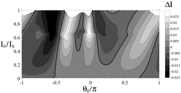
Figure 13: Plot representing variations of the action $\Delta I$ per ray cycle length for Model 2 under the noisy-like perturbation with $S_{0}(k)$ = const and $\varepsilon=0.005$. Bold lines correspond to zero variations of the action per ray cycle length.

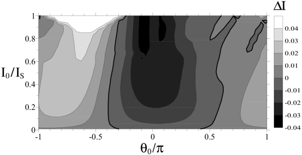
Figure 14: The same as in Fig. 13 but with $S_{0}(k)\propto k^{-2}$ and $\varepsilon=0.005$. Bold lines correspond to zero variations of the action per ray cycle length.

Consider now Model 2 with another kind of the perturbation spectrum, $S_{0}\propto k^{-2}$, and the same perturbation amplitude $\varepsilon=0.005$. In difference from the case with the flat spectrum, only one large “hill” now presents in Fig. 14 in the whole range of the action values. Moreover, the maximal variations of the action are larger as compared with the flat spectrum. One may conclude that under the noisy-like perturbation with the spectrum $S_{0}\propto k^{-2}$ the first harmonic in the series (98) is a dominant one in all the accessible phase space. The dependence $\Delta I(\vartheta_{0})$ is close to a cosine-like one.

Under a noisy-like perturbation, topology of the plots of variation of the action depends randomly on initial values of the time-like variable $r$, and this dependence is stronger in the case of the flat spectrum, especially in the range of large values of the action. It may cause not only phase shifts but even the number of “hills” and “hollows” may vary under varying initial values of $r$. In the case with decreasing spectral density, only smooth shifting of a “hill” along the $\vartheta$ axis may occur when varying initial values of $r$.

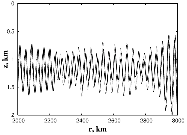
Figure 15: Two ray trajectories with starting momenta $p_{0}=-0.03$ (solid line) and $-0.02$ (dashed line) for Model 2 under the noisy-like perturbation with $S_{0}(k)\propto k^{-2}$.

VI.2 Coherent ray clusters

The plots of variations of the action allow us to treat the ray motion as a slow diffusion in the phase space between “hills” and “hollows”. If these “hills” (or “hollows”) are sufficiently large there may arise large fans of rays with close initial conditions preserving close current dynamical characteristics over long distances coherent ray clusters. In the ranges of strong variability of the phase space structure, phase correlations decay rapidly resulting in rapidly decaying clusters. So, the length of the phase correlations characterizes the stability of a cluster. Similar clusterization may occur in different physical systems (see, for example, Klyats ; Wolfs2 ). Therefore, the whole cluster structure may be considered as consisting of statistical and coherent parts. The rays, belonging to the statistical part, propagate in the same areas of the phase space with the same value of the Lagrangian ${\left<L\right>}$, do not correlate with each other and demonstrate exponential sensitivity to initial conditions. To the contrary, the rays in the coherent part do not show sensitive dependence on initial conditions. Two rays with initial values of the momentum $p_{0}=-0.02$ and $p_{0}=-0.03$ are shown in Fig. 15 in the range interval $r\in[2000:3000]$ km. The clusterization may influence strongly timefronts of sound signals. The prominent stripes visible in the timefront for the stochastic ray simulation (Fig. 16), which belong to ray clusters, resemble the respective strips visible in the timefront fragments for a deterministic perturbation (see Fig. 12a). It should be emphasized that similar strips have been found in the field experiments AET .

A decoherence and breaking of the respective coherent clusters become prominent with increasing the range (see fuzzy segments in Fig. 16b at the range $R=3000$ km). It is seen from Fig. 16d that late-arriving rays are registered not at the channel axis ($z_{a}\simeq 1$ km) but rather deeper, at $z\simeq 1.5$ km. Such a shift of the sound energy down in the depth may be explained as follows. The late-arriving signal is formed by a coherent cluster with near-axial rays deflected under propagation from the axial value of the action $I=0$. It follows from Eq. (67) that rays in this coherent cluster could arrive (at $R=3000$ km) at the depth different from $z_{a}$.

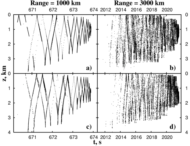
Figure 16: Timefronts for Model 2 under the noisy-like perturbation with (a,b) $S_{0}(k)$ = const and (c,d) $S_{0}\propto k^{-2}$. The ranges for the left and right plots are indicated in the figure.

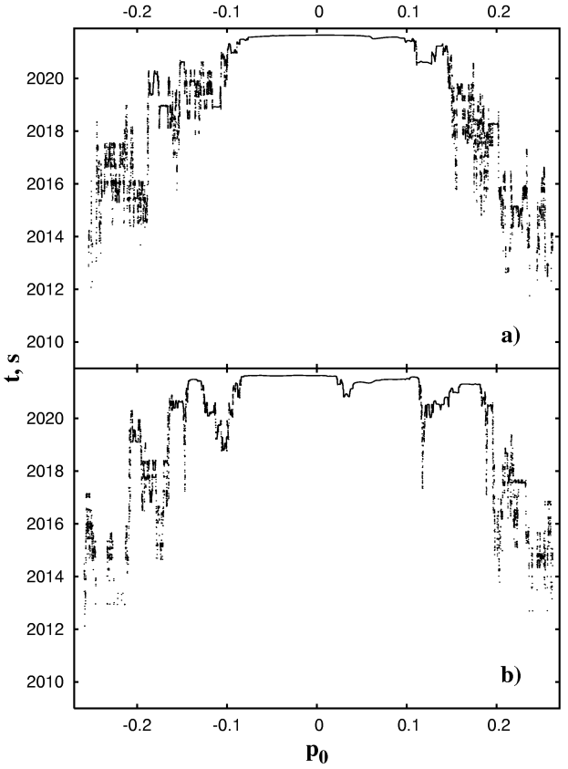
Figure 17: Ray travel time versus starting momentum for Model 2 under noisy-like perturbation with (a) $S_{0}(k)$ = const and (b) $S_{0}\propto k^{-2}$.

Figure 17 presents the ray travel time $t$ as a function of the starting ray momentum $p_{0}$ for Model 2 under the noisy-like perturbation with both the spectral models, $S_{0}(k)=$ const (a) and $S_{0}(k)\propto k^{-2}$ (b). All rays are chaotic under a noise perturbation, and one might naively expect to see randomly scattered points in the $t$–$p_{0}$ plots. In fact, we see in Fig. 17 smooth “shelf”-like segments alternating with unresolvable structures. Each “shelf” corresponds to a coherent cluster of rays. The “shelves” are distributed chaotically over the range of the starting momenta and their positions depend on a specific realization of the random process $\xi(r)$. Comparing between the two spectral models (Figs. 17a and b), we may conclude that the coherent cluster structure is more prominent with the spectral model $S_{0}(k)\propto k^{-2}$. Such a “shelf”-like structure has been found in $t(p_{0})$ plots for a model with a single-mode perturbation Smir , with “shelves” to be prescribed to regular islands in the respective phase space. The presence of “shelves” may complexify kinetic description of the ray motion with the help of a one-dimensional Fokker-Plank equation Viro-web ; Zas-PhA because the radius of phase correlations is not small in the presence of coherent clusterization.

VI.3 Periodic perturbation with a multiplicative noise superimposed

In the end of this section we consider a perturbation consisting of a periodic dependence of the sound-speed fluctuations on $r$ and a multiplicative noise superimposed

$$\xi(r)=(1-\alpha)\cos{\frac{2\pi r}{\lambda}}+\alpha\int\limits_{-\infty}^{\infty}S(k)e^{-ikr}\,dk,\quad 0\leq\alpha\leq 1,$$ (99)

where $\alpha$ is the strength of the noisy part. We have computed timefronts of sound signals at different values of $\alpha$. Fig. 9 shows function $F(t,\,R)$ with Model 1 at the fixed ranges $R=1000$ km and $R=3000$ km with the perturbation amplitude $\varepsilon=0.0025$ and spatial period $\lambda=10$ km corresponding to the Poincaré section in Fig. 5. The solid lines in Figs. 9–11 represent results at the range 1000 km with the lower axis showing the respective values of travel times, while the dashed lines are computed at the range 3000  km with the upper axis for travel times. As it expected, the amplitudes of the prominent peaks, caused by the nonlinear resonance with the periodic perturbation, decreases with increasing the values of $\alpha$. On the other hand, the amplitudes of the peaks in the late-arriving signal, caused by the noisy-like perturbation, increases with increasing $\alpha$.

Fig. 10 shows the function $F(t,\,R)$ for Model 1 under conditions of more strong chaos at increased value of the perturbation amplitude $\varepsilon=0.005$. All the “deterministic” peaks have comparatively small amplitudes even at $\alpha=0.5$. The distribution function $F(t,\,R)$ is shown for Model 2 in Fig. 11 with the same values of the parameters of perturbation as in the preceding figure with Model 1. It is seen that the peaks at $t\simeq 371.3$ s ($R=1000$ km) and at $t=2014$ s ($R=3000$ km), corresponding to the primary resonance of the first order $(l=1,\ m=5)$, disappear when the strength of noise reaches the magnitudes of the order $\alpha\geq 0.5$.

In difference from Model 1, coherent ray clusters in Model 2 appear not only in the late-arriving portion of the signal but, as well, in the early arriving portion corresponding to rays reflecting from the ocean surface. The rays with $H>H_{r}$ in Model 2 are less chaotic than the rays with $H<H_{r}$. These results show that ray dynamics is strongly influenced by the form of the background sound-speed profile. Depending on the form of the background profile, coherent ray clusters may appear in earlier, middle and later portions of a timefront. In our opinion, a stability in earlier portions of the wavefront to be measured in the field experiments Duda ; Worc3250 could be explained by peculiarities of the respective background sound-speed profile.

Under a deterministic perturbation with only a few frequencies, chaoticity of rays is defined mainly by the density of overlap of nonlinear resonances characterized by the Chirikov’s criterion (79) and is connected with the derivative of the frequency of spatial oscillations over the action $|\omega^{\prime}_{I}|$ (28). However, the Chirikov’s criterion is hardly applicable under conditions of a noisy-like perturbation with a large number of frequencies Beron-Vera ; Geoph . In this case we propose to use as a criterion of stochasticity the rate of decreasing of Fourier amplitudes in the series (98). Stochasticity of rays has been shown to become stronger if many terms present in the series (98). It can be used as a stochasticity criterion for nonlinear systems under a noisy-like perturbation in a close analogy with the Chirikov’s criterion for deterministic dynamical systems since the rate of decreasing of Fourier amplitudes is defined mainly by the dependence of the frequency of spatial oscillations $\omega$ on the action $I$. It is a linear function with Model 1 (26). In Model 2 the respective dependence $\omega(I)$ has a local maximum at $I_{r}\simeq I(H_{r})$. Thus, there arise conditions for forming coherent ray clusters in Model 2.

VII Conclusion

We have treated chaotic and stochastic nonlinear ray dynamics in underwater sound waveguides with longitudinal variations of the speed of sound caused by internal oceanic waves. Two models of sound-speed profiles, which are typical in shape for deep ocean sound channels, were designed analytically. We were managed to derive with them exact analytical solutions to the ray equations of motion without perturbation in terms of the depth-momentum and the action-angle variables and to find exact expressions for the frequency of spatial ray oscillations, the timefront of the sound signal at a fixed range and ray travel times. Three different kinds of internal-wave induced perturbations have been considered: a single-mode perturbation, a noisy-like multiplicative perturbation, and a periodic perturbation with a multiplicative noise superimposed.

We have found coherent clusters consisting of fans of rays with close dynamical characteristics over long distances and close arrival times. It is essential that forming the coherent clusters occurs under different kinds of perturbations, as periodic as noisy-like ones. The mechanism of their forming has been found to be connected with existence of specific zones of stability in the phase space of the perturbed system under consideration. In the case of a periodic perturbation, these zones appear due to ray-medium nonlinear resonances. In the case of a noisy-like multiplicative perturbation, zones of stability appear due to selective resonant interactions between different spectral components of the perturbation and harmonics of the unperturbed motion. As a result, the phase space has a specific “resonant” topology with local zones of stability. In order to visualize the topology, we have used the plots of variations of the action per ray cycle length.

We proposed a criterion for forming the coherent clusters, namely, the rate of decreasing of the Fourier amplitudes of a perturbation written in terms of the canonical action and angle variables. The effect of coherent clusterization depends on the horizontal spectrum of the field of internal waves as well. The clusterization becomes more prominent if the spectral density decreases rapidly with increasing the wave number $k$. The clusterization results in forming prominent peaks of functions of distribution of arrival times and manifests itself in timefronts of arriving signals as sharp strips on a smearing background formed by chaotic rays. It is worthwhile to stress that such strips have been found in timefronts measured in the field experiments AET . The clusterization may cause a redistribution of the acoustic energy over the depth, a stability of early arriving part of the sound signal and other effects. It should be taken into account in kinetic modelling of ray dynamics.

From the standpoint of acoustic tomography of the ocean, the coherent clusterization seems to be a useful property for the purpose of determining spatio-temporal variations of the hydrological characteristics on the real time scale under conditions of ray chaos. In a more general context, such a clusterization is interesting from the standpoint of general theory of influence of external multiplicative noise on Hamiltonian systems.

References

- (1) L.M. Brekhovskikh and Yu. Lysanov, Fundamentals of Ocean Acoustics (Springer-Verlag, Berlin, 1991).
- (2) S.S. Abdullaev and G.M. Zaslavsky, Zh. Eksp. Teor. Fiz. 80, 524 (1981) [Sov. Phys. JETP 53, 265 (1981)].
- (3) D.R. Palmer, M.G. Brown, F.D. Tappert, and H.F. Bezdek, Geophys. Res. Let. 15, 569 (1988).
- (4) S.S. Abdullaev and G.M. Zaslavsky, Usp. Fiz. Nauk 161, 1 (1991) [Sov. Phys. Usp. 34, 645 (1991)].
- (5) J.A. Colosi, S.M. Flatté, and C. Bracher, J. Acoust. Soc. Am. 96, 452 (1994).
- (6) J. Simmen, S.M. Flatté, and Guang-Yu Wang, J. Acoust. Soc. Am. 102, 239 (1997).
- (7) F.J. Beron-Vera, M.G. Brown, J.A. Colosi, S. Tomsovic, A.L. Virovlyansky, M.A. Wolfson, and G.M. Zaslavsky, e-print nlin.CD/0109027 (2002).
- (8) M.G. Brown, J.A. Colosi, S. Tomsovic, A.L. Virovlyansky, M.A. Wolfson, and G.M. Zaslavsky, J. Acoust. Soc. Am. 113, 2533 (2003).
- (9) M.A. Wolfson and F.D. Tappert, J. Acoust. Soc. Am. 107, 154 (2000).
- (10) T.F. Duda, S.M. Flatté, J.A. Colosi, B.D. Cornuelle, J.A. Hildebrand, W.S. Hodgkiss, P.F. Worcester, B.M. Howe, J.A. Mercer, and R.C. Spindel, J. Acoust. Soc. Am. 92, 939 (1992).
- (11) P.F. Worcester, B.D. Cornuelle, M.A. Dzieciuch, W.H. Munk, B.M. Howe, J.A. Mercer, R.C. Spindel, J.A. Colosi, K. Metzger, T.J. Birdsall, and A.B. Baggeroer, J. Acoust. Soc. Am. 105, 3185 (1999).
- (12) W.H. Munk and C. Wunsch, Deep-Sea Res. 26, 123 (1979).
- (13) V.A. Akulichev, V.P. Dzyuba, P.V. Gladkov, S.I. Kamenev, and Yu.N. Morgunov, in Theoretical and Computational Acoustics, edited by Er-Chang Shang, Qihu Li, and T.F. Gao (World Scientific, Singapore, 2002).
- (14) S.S. Abdullaev and G.M. Zaslavsky, Akust. Zh. 34, 578 (1988) [Sov. Phys. Acoust 34, 334 (1988)].
- (15) F.D. Tappert and Xin Tang, J. Acoust. Soc. Am. 99, 185 (1996).
- (16) I.P. Smirnov, A.L. Virovlyansky, and G.M. Zaslavsky, Phys. Rev. E 64, 1 (2001).
- (17) A.L. Virovlyansky, J. Acoust. Soc. Am. 113, 2523 (2003); e-print nlin. CD/0012015 (2002).
- (18) I.P. Smirnov, A.L. Virovlyansky, and G.M. Zaslavsky, Chaos 12, 617 (2002).
- (19) A. Iomin and G.M. Zaslavsky, Comm. Nonlin. Sci. Numer. Simul. 8, 401 (2003).
- (20) D.V. Makarov, M.Yu. Uleysky, and S.V. Prants, Tech. Phys. Lett. 29, 430 (2003).
- (21) L.D. Landau and E.M. Lifshitz, Mechanics (Nauka, Moscow, 1973).
- (22) D.V. Makarov, S.V. Prants, and M.Yu. Uleysky, Doklady Earth Science 382, 106 (2002).
- (23) K.B. Smith, M.G. Brown, and F.D. Tappert, J. Acoust. Soc. Am. 91, 1939 (1992); 91, 1950 (1992).
- (24) B.V. Chirikov, Phys. Rep. 52, 265 (1979).
- (25) G.M. Zaslavsky, M. Edelman, and B.A. Niyazov, Chaos 7, 159 (1997).
- (26) G.M. Zaslavsky and S.S. Abdullaev, Chaos 7, 182 (1997).
- (27) G.M. Zaslavsky, Physics of Chaos in Hamiltonian Systems (Academic Press, Oxford, 1998).
- (28) Yu.A. Kravtsov and Yu.I. Orlov, Geometrical Optics of Inhomogeneous Media (Springer, Berlin, 1990).
- (29) M.V. Budyansky, M.Yu. Uleysky, and S.V. Prants, Doklady Earth Science 387, 929 (2002).
- (30) M. Wiercigroch, A.H.-D. Cheng, J. Simmen, and M. Badiey, Chaos, Solitons & Fractals 9, 193 (1998).
- (31) C.J. Garrett and M.H. Munk, Geophys. Fluid Dyn. 2, 225 (1972); J. Geophys. Res. 80, 291 (1972).
- (32) F.J. Beron-Vera and M.G. Brown, e-print nlin. CD/0208038 (2002).
- (33) V.I. Klyatskin and D. Gurarie, Physics-Uspekhi 42, 165 (1999).
- (34) M.A. Wolfson and S. Tomsovic, J. Acoust. Soc. Am. 109, 2693 (2001).
- (35) M.G. Brown, Nonl. Proc. Geoph. 5, 69 (1998).