Exploring classical phase space structures of nearly integrable and mixed quantum systems via parametric variation

Abstract

The correlation between overlap intensities and level velocities has been introduced as a sensitive measure capable of revealing phase space localization. Previously applied to chaotic quantum systems, here we extend the theory to near-integrable and mixed quantum systems. This measure is useful in the latter cases because it has the ability to highlight certain phase space structures depending upon the perturbation used to parametrically vary the Hamiltonian. A detailed semiclassical theory is presented relating the correlation coefficient to the phase space weighted derivatives of the classical action. In the process, we confront the question of whether the Hannay-Ozorio de Almeida sum rules are simply extendable to mixed phase space systems. In addition, the $\hbar$-scalings of the correlation coefficient and relevant quantities are derived for nearly integrable systems. Excellent agreement is found between the theory and the results for integrable billiards as well as for the standard map.

I Introduction

System response to parametric variations or perturbations is of great importance. It is a powerful experimental practice from which new information about a system can be extracted that is not generally available by other means, especially for complex systems, i.e. disordered, interacting many-body, and/or simple chaotic systems. External parameters such as electromagnetic fields, temperatures, applied stresses, etc., are controllable and often suitable for this purpose. Some specific examples include conductance fluctuations in quantum dots quantumdots , and variations in eigenmodes due to shape deformations of microwave cavities sridhar:94 and vibrating plates schaadt:99 . Intramolecular vibarational energy redistribution gruebele:00 in molecules is another example wherein the technique of parametric variations can lead to useful insights regarding the key perturbations responsible for strong mode mixings. Molecular spectroscopy in external fields is an area of current interest and the response of a molecular system to external fields can be usefully analyzed from the parametric perspectives fraser:94 .

In the extreme chaotic or disordered limit, there exist universalities in system response to perturbations simon:93 , and the eigenstates respect the ergodic hypothesis berry:77 , i.e. no phase space localization; there is only a scale to extract. On the other hand, the response of integrable or near-integrable systems is far richer being system dependent, and the Husimi distributions of the eigenstates are confined to classical tori takahashi:86 ; kurchan:89 . A perturbation is likely to give rise to subsets of eigenlevels/states that respond very similarly as a group, and the parametric quantities thereby carry far more information. For mixed systems both regular and chaotic trajectories form phase space structures and the most obvious, naive initial starting point would be to attempt to analyze each structure separately. At this level of approximation, using the appropriate semiclassical theory for regular and chaotic regions involves the respective integrable and chaotic Hannay-Ozorio de Almeida sum rule expressions hannay:84 weighted by the relative fractions of phase space volume. We find instead that the intermittent behavior of the unstable orbits prevents this simple picture from applying.

A measure was introduced by one of us (S.T.) tomsovic:96 that reveals phase space localization of quantum eigenstates. Originally introduced for chaotic systems, the measure correlates the changes in the eigenenergies due to a perturbation (termed “level velocities”) with the overlap intensities between the eigenstates and a probe state, which is often usefully chosen to be a coherent state. More recently, it has been identified as contributing to the scale associated with the fidelity in the weak perturbative regime ct2 . For integrable systems phase space localization is the norm, not the exception. There and in the near-integrable regime, the localization is associated with tori, resonance zones and stable periodic orbits. The correlation measure has been shown to highlight different features of classical phase space depending upon the perturbation keshavamurthy:02 . Several years ago Weissman and Jortner weissman:82 performed a similar study involving the Husimi distributions and parametric changes in eigenenergy levels.

This paper is organized as follows: we begin by developing the semiclassical theory of the correlations for near-integrable systems where we also remark on the more general theory for the level velocities in mixed systems. The correlations have been previously studied in highly excited rovibrational states in molecules where multiresonant Hamiltonians are applicable keshavamurthy:02 . Section III gives the semiclassical theories of the level velocities, strength functions and overlap intensity-level velocity correlation coefficients. The semiclassical theory is compared with various results from integrable billiards and the standard map which has the entire range of dynamics from integrable to fully chaotic. We finish with a discussion of the similarities and distinctions between near-integrable and chaotic systems and some comments about mixed systems.

II Preliminaries

Consider a near-integrable quantum system governed by a smoothly parameter-dependent Hamiltonian $\hat{H}(\lambda)$ with classical analog $H({\bf I},{\bm{\theta}};\lambda)$ where

$$H({\bf I},{\bm{\theta}};\lambda)=H_{0}({\bf I})+\lambda H_{1}({\bf I},{\bm{\theta}})$$ (1)

Without loss of generality, the phase space volume of the energy surface, $V$, is taken to be a constant as a function of $\lambda$. This ensures that the eigenvalues do not collectively drift in some direction in energy, but rather wander locally. The parameterized strength function is given by

$$S_{\alpha}(E,\lambda) = {1\over 2\pi\hbar}\int^{\infty}_{-\infty}e^{iEt/\hbar}\langle\alpha|e^{-i\hat{H}(\lambda)t/\hbar}|\alpha\rangle dt$$ (2)

$$= \sum_{n}p_{\alpha n}(\lambda)\delta(E-E_{n}(\lambda))$$

where $p_{\alpha n}(\lambda)=|\langle\alpha|E_{n}(\lambda)\rangle|^{2}$. $S_{\alpha}(E,\lambda)$ is the Fourier transform of the autocorrelation function of a normalized initial state $|\alpha\rangle$. Ahead $\overline{S}_{\alpha}(E,\lambda)$ will denote the smooth part resulting from the Fourier transform of just the extremely rapid initial decay due to the shortest time scale of the dynamics (zero-length trajectories). We will take $|\alpha\rangle$ to be a Gaussian wave packet because of its ability to probe ‘quantum phase space’, but other choices may be useful depending on the circumstances. In one spectroscopic application, we found it to be advantageous to take $|\alpha\rangle$ as a momentum state keshavamurthy:02 .

The overlap intensity-level velocity correlation coefficient is defined as

$${\cal C}_{\alpha}(\lambda)\equiv{\left\langle p_{\alpha n}{\partial E_{n}(\lambda)\over\partial\lambda}\right\rangle_{E}\over\sigma_{\alpha}\sigma_{E}}$$ (3)

where $\sigma^{2}_{\alpha}$ and $\sigma^{2}_{E}$ are the local variances of intensities and level velocities, respectively. The brackets denote a local energy average in the neighborhood of $E$. It weights most the level velocities whose associated eigenstates possibly share common localization characteristics and measures the tendency of these levels to move in a common direction. In this expression, the phase space volume remains constant so that the level velocities are zero centered (otherwise the mean must be subtracted), and ${\cal C}_{\alpha}(\lambda)$ is rescaled to a unitless quantity with unit variance making it a true correlation coefficient. The set of states included in the local energy averaging can be left flexible except for a few constraints. Only energies where $\overline{S}_{\alpha}(E,\lambda)$ is roughly a constant can be used or some intensity unfolding must be applied. The energy range must be small so that the classical dynamics are essentially the same throughout the range, but it must also be broad enough to include enough eigenstates for statistical purposes.

III Semiclassical Dynamics

We develop a theory based upon semiclassical dynamics for the overlap correlation coefficient of regular states by examining its individual components, the level velocities and intensities. The theory for the variance of the level velocities involves the trace formula for near-integrable systems developed by Ullmo, Grinberg and Tomsovic ullmo:96 . The near-integrable trace formula is used rather than the simpler integrable trace formula of Berry and Tabor berrytabor:77 since it correctly describes the contributions of short, unstable periodic orbits that occur after a system breaks integrability. The level velocities are derivatives and thus far more sensitive to the perturbation than the intensities. Hence, it is more important to accurately describe the level velocities. The intensity variances for near-integrable systems are given by the integrable result as long as the coherent state is not near a resonance zone.

It turns out that a general result for the level velocity variance in mixed systems cannot be obtained simply by applying the appropriate Hannay-Ozorio de Almeida sum rule for the effectively regular and chaotic trajectories separately. The “effective” trajectories are not easily defined since they do not merely correspond to the trajectories within the KAM islands and the chaotic sea, respectively. Although, it is observed that the near-integrable result for the level velocities is in good agreement with the calculated results before the break up of the last KAM torus.

III.1 Level velocities

By adapting a method employed by Berry and Keating berry:94 for classical chaotic systems with the topology of a ring threaded by quantum flux and later generalized for all continuous time chaotic systems leboeuf:99 ; cerruti:01 , the variance of the level velocities can be obtained. The details for near-integrable systems are in appendix A where the variance of the level velocities is found to be

$$\sigma^{2}_{E} \approx {4\pi\epsilon\over V\hbar}\sum_{\bf M}{}^{\prime}\left\langle A_{\bf M}^{2}\left\{\left(\partial\overline{S}_{\bf M}\over\partial\lambda\right)^{2}[J_{0}^{2}(s_{\lambda})+\tilde{a}^{2}J_{1}^{2}(s_{\lambda})]\right.\right.$$ (4)

$$+ \left.\left(\partial\Delta S_{\bf M}\over\partial\lambda\right)^{2}\left[{\tilde{a}^{2}\over 4}(J_{0}(s_{\lambda})-J_{2}(s_{\lambda}))^{2}+J_{1}^{2}(s_{\lambda})\right]\right\}$$

$$\times \left.\exp\left({-2\epsilon T_{\bf M}\over\hbar}\right)\right\rangle_{E}$$

where the $\epsilon\rightarrow 0$ limit is understood, and the amplitude factor is determined by the integrable system, $H_{0}({\bf I})$

$$A_{\bf M}={1\over 2\pi|{\bf M}|^{(d+1)/2}\sqrt{|K_{\bf M}|}}$$ (5)

The prime on the sum excludes the ${\bf M}=0$ term. ${\bf M}$ labels the rational tori and is a $d$-dimensional vector with positive integer components whose classical paths are those which at time $t$ have returned to the same point on their torus after making $M_{1}$ circuits of coordinate $\theta_{1}$, $M_{2}$ circuits of coordinate $\theta_{2}$, etc. berrytabor:77 . $K_{\bf M}$ is the scalar curvature matrix of the energy contour and $T_{\bf M}$ is the period of the unperturbed orbit on the resonant torus. $J_{0}(z)$ and $J_{1}(z)$ are the standard Bessel functions. By the Poincaré-Birkhoff theorem only two periodic orbits survive the break-up of a rational torus. One orbit is stable and the other is unstable with actions $S_{s}$ and $S_{u}$ and stability matrices $M_{s}$ and $M_{u}$, respectively. Hence, we define

$$\overline{S}_{\bf M}(\lambda)\equiv{S_{u}+S_{s}\over 2}\ \ \ \mathrm{and}\ \ \ \Delta S_{\bf M}(\lambda)\equiv{S_{u}-S_{s}\over 2}$$ (6)

with $s_{\lambda}=\Delta S_{\bf M}(\lambda)/\hbar$ and

$$\tilde{a}(\lambda)\equiv{\kappa-1\over\kappa+1}$$ (7)

where

$$\kappa=\left(-{\det(M_{u}-{\bf 1})\over\det(M_{s}-{\bf 1})}\right)^{1/2}$$ (8)

In the case $\kappa\rightarrow 1$ then $\tilde{a}(\lambda)\rightarrow 0$ and the spectral staircase reduces to Ozorio de Almeida’s result ozorio:86 .

The summation over rational tori can be accomplished by applying the Hannay-Ozorio de Almeida sum rule for integrable systems hannay:84

$$\sum_{\bf M}{}^{\prime}A_{\bf M}^{2}\cdots\rightarrow{V\over 2\pi}\int{dT\over T^{2}}\cdots$$ (9)

Thus,

$$\sigma^{2}_{E}\approx{2\epsilon\over\hbar}\int{1\over T^{2}}\left\langle\left\{\left(\partial\overline{S}_{\bf M}\over\partial\lambda\right)^{2}[J_{0}^{2}(s_{\lambda})+\tilde{a}^{2}J_{1}^{2}(s_{\lambda})]\right.\right.$$

$$+\left.\left.\left(\partial\Delta S_{\bf M}\over\partial\lambda\right)^{2}\left[{\tilde{a}^{2}\over 4}(J_{0}(s_{\lambda})-J_{2}(s_{\lambda}))^{2}+J_{1}^{2}(s_{\lambda})\right]\right\}\right\rangle_{\bf M}$$

$$\times\exp\left({-2\epsilon T\over\hbar}\right)dT$$ (10)

For rational tori, the change of the classical action is proportional to the period of motion. We can think of this as a “ballistic” action change in contrast to the diffusive action changes of chaotic trajectories. The variance is therefore proportional to the square of the period. According to the numerical calculations discussed ahead, ballistic action changes hold equally well for integrable and near-integrable systems, but this is not true for mixed phase space systems. Thus, excluding mixed systems,

$$\left\langle\left\{\left(\partial\overline{S}_{\bf M}\over\partial\lambda\right)^{2}[J_{0}^{2}(s_{\lambda})+\tilde{a}^{2}J_{1}^{2}(s_{\lambda})]\right.\right.$$

$$+\left.\left.\left(\partial\Delta S_{\bf M}\over\partial\lambda\right)^{2}\left[{\tilde{a}^{2}\over 4}(J_{0}(s_{\lambda})-J_{2}(s_{\lambda}))^{2}+J_{1}^{2}(s_{\lambda})\right]\right\}\right\rangle_{\bf M}$$

$$=\zeta(E,\lambda;\hbar)T^{2}$$ (11)

It was shown in ullmo:96 that the expression involving Bessel functions collapsed to the usual Berry-Tabor expression for most tori (with a minor adjustment for the slight distortion of the torus, i.e. $s_{\lambda}=0,\partial\Delta S_{\bf M}/\partial\lambda=0$). Only very slowly as $\hbar\rightarrow 0$, did tori other than those possessing the lowest order ${\bf M}$ require the Bessel function weightings. For these higher order tori, Eq. (III.1) is understood as being just the mean square of $\partial\overline{S}_{\bf M}/\partial\lambda$.

Performing the integral, the variance of the level velocities becomes simply

$$\sigma^{2}_{E}\approx\zeta(E,\lambda;\hbar)$$ (12)

which is only very weakly dependent on $\hbar$ for those low order tori requiring the Bessel function weightings. Thus, in the integrable limiting case, the $\hbar$-dependence disappears altogether.

For mixed phase space systems, the question is whether a generalization of Eqs. (9,III.1) is possible; for the fully chaotic case, the expressions are modified by replacing $T^{2}$ by $T$ and the coefficients change. Is it possible to have fractionally weighted parts of both expressions? First, instead of summing over rational tori $\bf M$, the sum is considered over all periodic orbits. Given the diffusive action change behavior for fully chaotic systems and ballistic for regular systems, conceptually, the full set of action changes might decompose into a linear and a quadratic component. Continuing with this logic, Eq. (9) would apply for the periodic orbits with ballistic action changes and be weighted by the appropriate fraction of phase space volume. It is important to note a couple of subtleties here. Both a stable and unstable orbit combined to define $\{\overline{S}_{\bf M},\Delta S_{\bf M}\}$. Thus, the quadratic and linear components cannot be as simple as treating the stable orbits ballistically and the unstable orbits diffusively. Perhaps, at least as many orbits with positive Lyapunov exponent as stable orbits should be treated ballistically. Secondly, the key ingredient, $\overline{S}_{\bf M}$, is the average of said stable and unstable orbit actions. Taking the mean square of the sum of two orbits’s actions is equal to the square of the sum only if the action changes are nearly equal. Excluding the lowest order tori, this does turn out to be roughly true.

Similarly, the remaining unstable orbits would be treated with the appropriate (chaotic) versions of Eqs. (9,III.1). With this separation, the proposition would be that the level velocity variance is the sum of the near-integrable result and the previously derived chaotic result cerruti:01 ,

$$\sigma^{2}_{E}\approx\zeta(E,\lambda;\hbar)f+{gK(E,\lambda)\hbar^{d-1}\over\pi V}(1-f)$$ (13)

where $f$ is the fraction of ballistically-behaving orbits, and $g$ is a symmetry factor for the system. The quantities $\zeta(E,\lambda;\hbar)$ and $K(E,\lambda)$ would be determined by the ballistic and diffusive versions of Eq. (III.1), respectively. The section on the kicked rotor will address this issue.

III.2 Overlap intensities

Next, the overlap intensities are investigated and a semiclassical derivation of their variance is obtained. For an integrable system the overlap intensities are best expressed in action-angle coordinates; details are in appendix B and the result is

$$\sigma^{2}_{\alpha}\approx{\prod\sigma^{2}_{j}\over\pi^{d}}\left\langle\exp\left[{-2(\Delta{\bf I})^{2}\over\hbar^{2}}\right]\right\rangle_{\bf M}$$ (14)

where in the exponential argument of the wave packet, each component is $(\Delta{\bf I})_{j}\equiv\sigma_{j}({\bf I}-{\bf I}_{\alpha})_{j}$. The variance is a Gaussian weighted average of the action of the wave packet over the rational tori.

The Gaussian weighting can be evaluated by replacing the $\bf{M}$ averaging by an average of the action variables over the energy surface

$$\left\langle\exp\left[{-2(\Delta{\bf I})^{2}\over\hbar^{2}}\right]\right\rangle_{\bf M} \approx {(2\pi)^{d}\over V}\int\exp\left[{-2(\Delta{\bf I})^{2}/\hbar^{2}}\right]$$ (15)

$$\times\delta(E-H_{0}({\bf I}))d{\bf I}$$

The Hamiltonian in the numerator is expanded about ${\bf I}_{\alpha}$ giving

$$H_{0}({\bf I})=H_{0}({\bf I_{\alpha}})+{\bm{\omega}}_{\alpha}\cdot({\bf I}-{\bf I}_{\alpha})+\cdots$$ (16)

where $H_{0}({\bf I_{\alpha}})=E$ and ${\bm{\omega}}_{\alpha}=\partial H_{0}({\bf I_{\alpha}})/\partial{\bf I}$. Only linear terms are necessary in the semiclassical limit as long as each width component is chosen such that $\sigma_{j}/\hbar\rightarrow\infty$ as $\hbar\rightarrow 0$; we take $\sigma_{j}\propto\hbar^{1/2}$ so that uncertainty in ${\bf I}$ and ${\bf\theta}$ shrink similarly as $\hbar$ shrinks. After performing the integration of the weighting over the energy shell, the result is

$$\left\langle\exp\left[{-2(\Delta{\bf I})^{2}\over\hbar^{2}}\right]\right\rangle_{\bf M} \approx \left({\pi\hbar^{2}\over 2}\right)^{(d-1)/2}$$ (17)

$$\times {1\over V\prod\sigma_{j}\sqrt{\sum\left({\omega_{\alpha j}/\sigma_{j}}\right)^{2}}}$$

which has an $\hbar$-scaling of $\hbar^{(d-1)/2}$. Therefore, the leading order $\hbar$-scaling for the intensity variance for near-integrable systems is

$$\sigma^{2}_{\alpha}={\prod\sigma_{j}\over V\sqrt{\sum\left({\omega_{\alpha j}/\sigma_{j}}\right)^{2}}}\propto\hbar^{(3d-1)/2}$$ (18)

III.3 Correlations

Finally, the semiclassical theories for the overlap intensities and the level velocities outlined above can now be used to construct the correlation function. Beginning with the covariance, it can be shown that

$$Cov_{\alpha}(\lambda) = \left\langle p_{\alpha n}(\lambda){\partial E_{n}(\lambda)\over\partial\lambda}\right\rangle_{n}$$ (19)

$$= {2\pi h^{d}\epsilon\over V}\left\langle S_{\alpha}(E;\lambda){\partial N(E;\lambda)\over\partial\lambda}\right\rangle_{E}$$

The semiclassical expressions for the strength function and the parametric derivative of the staircase function give

$$Cov_{\alpha}(\lambda)={-\epsilon 2^{(d+3)/2}\prod\sigma_{j}\pi^{1/2}\over V\hbar}$$ (20)

$$\times \left\langle\sum_{\bf M}{}^{\prime}|A_{\bf M}||D_{s}|^{1/2}\left[\left(\partial\overline{S}_{\bf M}\over\partial\lambda\right)[J_{0}(s_{\lambda})-i\tilde{a}(\lambda)J_{1}(s_{\lambda})]\right.\right.$$

$$+ \left.i\left(\partial\Delta S_{\bf M}\over\partial\lambda\right)\left(J_{1}(s_{\lambda})+{i\tilde{a}(\lambda)\over 2}[J_{0}(s_{\lambda})-J_{2}(s_{\lambda})]\right)\right]$$

$$\times \left.\exp\left(-{(\Delta{\bf I})^{2}\over\hbar^{2}}-{2\epsilon T_{\bf M}\over\hbar}\right)\right\rangle_{E}$$

Again, the diagonal approximation has been made in the above expression. Following arguments parallel to those in deriving the variances leads to the expression

$$Cov_{\alpha}(\lambda) = {-2\prod\sigma_{j}\over\pi^{d/2}\tau_{H}}\int{dT\over T}e^{-2T/\tau_{H}}$$ (21)

$$\times\left\langle\left({\partial S_{\bf M}\over\partial\lambda}\right)\exp\left[{-(\Delta{\bf I})^{2}\over\hbar^{2}}\right]\right\rangle_{\bf M}$$

for integrable systems where $\tau_{H}=\hbar/\epsilon$ is the Heisenberg time.

In order to make further progress in understanding the correlation function, it is necessary to know the time dependence of the ${\bf M}$-averaged expression. It is important to note that the Gaussian weighting factor will not decouple from the parametric action derivative at long times and thus, the local average of the derivatives of the action is not necessarily zero. The weighted action derivatives can be approximated by the same method as used in the calculation the variance of the level velocities, so for integrable systems

$$\left\langle\left({\partial S_{\bf M}\over\partial\lambda}\right)\exp\left[{-(\Delta{\bf I})^{2}\over\hbar^{2}}\right]\right\rangle_{\bf M}$$

$$\approx{\int(\partial S_{\bf M}/\partial\lambda)\exp[-(\Delta{\bf I})^{2}/\hbar^{2}]\delta(T-T_{\bf M})d{\bf M}\over\int\delta(T-T_{\bf M})d{\bf M}}$$

$$\approx T\xi(\lambda)$$ (22)

Note that the above average is linear with the period. The $\hbar$-scaling of $\xi(\lambda)$ is the same as for the average Gaussian weighting in the previous subsection which is $\hbar^{(d-1)/2}$.

The final result of the covariance is

$$Cov_{\alpha}(\lambda)\approx{-\xi(\lambda)\prod\sigma_{j}\over\pi^{d/2}}$$ (23)

Combining this with the results above for the variances generates the semiclassical expression for the correlation function

$${\cal C}_{\alpha}(\lambda)\approx{-\xi(\lambda)\over\zeta^{1/2}(E,\lambda)\left\langle\exp\left[-2(\Delta{\bf I})^{2}/\hbar^{2}\right]\right\rangle^{1/2}_{\bf M}}$$ (24)

where the expectation value is evaluated in Eq. (17). For near-integrable systems in the semiclassical limit, the above result implies that $Cov_{\alpha}(\lambda)\propto\hbar^{(2d-1)/2}$ whereas the correlation ${\cal C}_{\alpha}(\lambda)\propto\hbar^{(d-1)/4}$ to leading order.

IV Results

IV.1 Rectangular and box billiards

First, we consider billiards that are totally separable in Cartesian coordinates and thus completely integrable. These types of billiards have been used in the study of spectral rigidity berry:85 . In particular, we examine a rectangular billiard with sides $a,b$ and a box billiard with sides $a,a,b$; the sidelength $a$ is varied. The density of states is kept constant by not changing the area ${\cal A}$ of the rectangle or the volume ${\cal V}$ of the box. The action/angle variables are proportional to the momentum/position coordinates in each direction,

$$I_{j}=\ell_{j}p_{j}/\pi\ \ \ \mbox{and}\ \ \ \theta_{j}=\pi q_{j}/\ell_{j}$$ (25)

where $\ell_{j}$ is the side length of the $j$th side. The Hamiltonians are given by

$$H({\bf I})={\pi^{2}\over 2m}\sum_{j}\left({I^{2}_{j}\over\ell^{2}_{j}}\right)$$ (26)

The classical action of the rectangle for a closed orbit on a given resonant torus ${\bf M}$ is

$$S_{\bf M}=\sqrt{8mE}[M^{2}_{1}a^{2}+M^{2}_{2}({\cal A}/a)^{2}]^{1/2}$$ (27)

the period is

$$T_{\bf M}=\sqrt{2m[M^{2}_{1}a^{2}+M^{2}_{2}({\cal A}/a)^{2}]/E}$$ (28)

and the derivative of the action along the orbit is

$${\partial S_{\bf M}\over\partial a}={\sqrt{8mE}\over a}{M^{2}_{1}a^{2}-M^{2}_{2}({\cal A}/a)^{2}\over[M^{2}_{1}a^{2}+M^{2}_{2}({\cal A}/a)^{2}]^{1/2}}$$ (29)

Similarly, the classical action of the box is

$$S_{\bf M}=\sqrt{8mE}[(M^{2}_{1}+M^{2}_{2})a^{2}+M^{2}_{3}({\cal V}/a^{2})^{2}]^{1/2}$$ (30)

the period is

$$T_{\bf M}=\sqrt{2m[M^{2}_{1}a^{2}+M^{2}_{2}a^{2}+M^{2}_{3}({\cal V}/a^{2})^{2}]/E}$$ (31)

and the derivative of the action is

$${\partial S_{\bf M}\over\partial a}={\sqrt{8mE}\over a}{(M^{2}_{1}+M^{2}_{2})a^{2}-2M^{2}_{3}({\cal V}/a^{2})^{2}\over[(M^{2}_{1}+M^{2}_{2})a^{2}+M^{2}_{3}({\cal V}/a^{2})^{2}]^{1/2}}$$ (32)

Using the above quantities and performing the integration in Eq. (III.1), the variance of the action derivatives are $2E^{2}T^{2}/a^{2}$ and $16E^{2}T^{2}/5a^{2}$ for the rectangle and the box, respectively. Hence, the respective values of $\zeta(E,a)$ are $2E^{2}/a^{2}$ and $16E^{2}/5a^{2}$, which approach the variances of the level velocities in the semiclassical limit. Figure 1 demonstrates how well $\zeta(E,a)$ approximates the level velocities especially as $\hbar\rightarrow 0$. Note that the level velocities are virtually independent of $\hbar$ as predicted.

Figure 1: Variance of the level velocities for rectangular and box billiards. The area and volume are taken to be unity, while the sidelength $a=1.1$; the energy is 600. The upper panel is for the rectangle and the lower panel is for the box. The solid line is the quantum results while the dashed line is the semiclassical theory.

The $\hbar$-scaling of the intensity variance is predicted to be $\hbar^{5/2}$ and $\hbar^{4}$, respectively, for the rectangular and box billiards. Using Eq. (17) with $\omega_{\alpha,j}=\pi^{2}I_{\alpha,j}/m\ell^{2}_{j}$ the semiclassical theory and quantum intensity variances are compared in Fig. 2. The agreement is quite good as $\hbar\rightarrow 0$.

Figure 2: Variance of the intensities for the rectangular and box billiards. The area and volume are taken to be unity, while the sidelength $a=1.1$; the energy is 600. The upper panel is for the rectangle and the lower panel is for the box. The solid line is the quantum results while the dashed line is the semiclassical theory.

The last two quantities, the covariance and correlation, are shown in Fig. 3 and Fig. 4, respectively, along with the results from the semiclassical theory. The values of $\xi(E,a)$ are obtained from Eq. (III.3). For the rectangle

$$\xi(E,a)={2\pi^{3/2}\hbar\over am\sigma\sqrt{2mE}}\left({I^{2}_{\alpha,1}\over a^{2}}-{I^{2}_{\alpha,2}\over({\cal A}/a)^{2}}\right)$$ (33)

and for the box

$$\xi(E,a)={\pi^{2}\hbar^{2}\over am^{2}E\sigma^{2}}\left({I^{2}_{\alpha,1}\over a^{2}}+{I^{2}_{\alpha,2}\over a^{2}}-{2I^{2}_{\alpha,3}\over({\cal V}/a^{2})^{2}}\right)$$ (34)

The agreement is excellent in both cases. Note that we have used no fitting parameters in any of the figures in these subsection.

Figure 3: Covariance for the rectangular and box billiards. The area and volume are taken to be unity, while the sidelength $a=1.1$; the energy is 600. The upper panel is for the rectangle and the lower panel is for the box. The solid line is the quantum results while the dashed line is the semiclassical theory.

Figure 4: Correlation for the rectangular and box billiards. The area and volume are taken to be unity, while the sidelength $a=1.1$; the energy is 600. The upper panel is for the rectangle and the lower panel is for the box. The solid line is the quantum results while the dashed line is the semiclassical theory.

IV.2 Standard map

In this subsection we compare the semiclassical theories to the numerical results for the standard map. The classical standard map is defined by

$$q_{i+1} = q_{i}+p_{i+1}\ \ \mathrm{mod}(1)$$

$$p_{i+1} = p_{i}-(k/2\pi)\sin(2\pi q_{i})\ \ \mathrm{mod}(1)$$ (35)

where the “kicking strength” $k$ is the varied parameter. The map displays the entire range of classical dynamics from integrable at $k=0$ to fully chaotic beyond $k\approx 5$.

Instead of the velocities of the eigenvalues of the Hamiltonian, it is the velocities of the eigenangles for the standard map which are of interest. The matrix elements of the quantum map with $N$ discrete levels can be written al:97

$$\langle n|U|n^{\prime}\rangle = {1\over\sqrt{iN}}\exp[i\pi(n-n^{\prime})^{2}/N]$$ (36)

$$\times\exp\left(i{kN\over 2\pi}\cos[2\pi(n+a)/N]\right)$$

where $n,n^{\prime}=0,\dots,N-1$; $a$ is a phase term which we set equal to zero. The effective Planck constant is given by $h=1/N$. The eigenvalues of the propagator are $U|\psi_{j}\rangle=\exp(-i\phi_{j})|\psi_{j}\rangle$ with real eigenangles $\phi_{j}$. The “level velocities” are given by the Hellmann-Feynman theorem

$${d\phi_{j}\over dk}={N\over 2\pi}\langle\psi_{j}|\cos(2\pi q)|\psi_{j}\rangle$$ (37)

The smoothed density of states for the eigenangles oconnor:91 is

$$d_{\epsilon}(\phi)={N\over 2\pi}+{1\over 2\pi}\sum^{\infty}_{n=-\infty}\exp(in\phi)\mathrm{Tr}\,U^{n}\exp(-n\epsilon)$$ (38)

where the sum excludes $n=0$ and the trace of the propagator in the integrable regime is

$$\mathrm{Tr}\,U^{n}=\sum_{\bf M}\sqrt{N\over in}\exp(2\pi iNS_{\bf M})$$ (39)

Integrating over the angle, the smoothed spectral staircase is

$$N_{\epsilon}(\phi) = {N\phi\over 2\pi}-{1\over 2\pi}\sum^{\infty}_{n=-\infty}\sum_{\bf M}{1\over n}\sqrt{iN\over n}\exp(in\phi)$$ (40)

$$\times\exp(2\pi iNS_{\bf M})\exp(-n\epsilon)$$

The resonant tori ${\bf M}$ including repetitions for the standard map are given by a constant momentum equal to the rational fraction $m/n$ where $m=0,\dots,n-1$ and $n$ is the period of the torus. The derivative of the action with respect to the kicking strength is

$${\partial S_{\bf M}\over\partial k}={1\over(2\pi)^{2}}\sum^{n}_{i=1}\cos(2\pi q_{i})$$ (41)

For the integrable case ($k=0$), the periodic points are $q_{i}=q_{0}+m\cdot i/n\ \ \mathrm{mod}(1)$ and hence, $\partial S_{\bf M}/\partial k=0$ for all resonant tori. Thus, by Eqs. (III.1) and (12) the variance of the level velocities is zero.

In the near-integrable regime, the variance of the eigenangles is approximately given by the result

$$\sigma^{2}_{\phi}\approx 4\pi^{2}\zeta N^{2}$$ (42)

Note that the eigenangles are divided by an effective $\hbar$ making the variance of the eigenangles quadratic in $N$. We do not have an analytic formula for $\zeta$, but it can be obtained numerically from the quadratic period dependence of the variance of the action derivatives averaged over the tori. For $k=0$, it is straightforward to calculate analytically the positions of the stable and unstable periodic orbits that arise as soon as integrability is broken. Curiously, using these points as initial conditions for the periodic orbits throughout the near-integrable regime, roughly $k\in[0,2]$, gives results within a few percent of that found by locating the true periodic orbits. In order to make long time calculations, this compromise is indispensable and does not harm the approximation noticeably. In Fig. 5, the near-integrable theory is shown to give excellent agreement with the quantum eigenangle velocity variance even though there exists a significant proportion of unstable orbits for the larger values of $k$ shown that are being treated as though they were stable.

Figure 5: The variance of the level velocities for the standard map ($N=500$). The solid line is the quantum results while the dashed line is the semiclassical theory using the near-integrable results of Eq. (42).

In the mixed regime, the corresponding proposition of Eq. (13) is

$$\sigma^{2}_{\phi}\approx 4\pi^{2}\zeta(k)fN^{2}+g{D(k)\over 4\pi^{2}}(1-f)N$$ (43)

where $g=4$ and $D(k)$ is the classical action diffusion constant. It was shown previously lakshminarayan:99 that a direct method based on classical orbits gave a good correspondence between the theory and quantum values for

$$\sigma^{2}_{\phi} \approx {N^{2}\over 4\pi^{2}}\int^{1}_{0}\int^{1}_{0}V(q_{0})\langle V(q^{(n)}(q_{0},p_{0}))\rangle_{n}dp_{0}dq_{0}$$ (44)

$$\approx c_{1}(k)N+c_{2}(k)N^{2}$$

where $V(q)=\cos(2\pi q)$ but no understanding was given of the two coefficients. Equation (43) gives one plausible, but naive, interpretation.

In order to test numerically the separation of diffusive and ballistic contributions in the mixed regime, it is impossible to work with the periodic orbits. They proliferate exponentially and must be found numerically. The time over which this can be done by brute force calculation is too short for our purposes. Instead, a Monte Carlo technique is needed. We have devised a method that begins with a uniform sampling of initial conditions in the phase space, and relies on the properties of finite time Lyapunov exponents grassberger:88 . Although, a stable periodic orbit has a vanishing Lyapunov exponent, at a partial period of its motion, the trace, $Q$, of its stability matrix can grow as a power of the propagation time. This can give a stable orbit the appearance of being unstable depending on circumstances. For example, constructing a surface of section based on whether $|Q|<2$ fails miserably. If instead, one seeks the least square deviation of the time development of $Q$ from the form

$$\bar{Q}=aT^{\gamma}\exp\mu T$$ (45)

then the estimate of the Lyapunov exponent can be used to judge whether an orbit is in the stable or unstable part of the phase space; i.e. the construction of the correct surface of section is recovered in this way.

Figure 6 gives a histogram of the finite time Lyapunov exponents, $\mu$, calculated using Eq. (45) for the orbits in this regime. The orbits are separated into three rough categories depending upon their stabilities as mentioned in the previous section. The broadened $\delta$-function feature near zero represents the stable orbits that have action derivatives with a quadratic dependence upon time. The set of most highly unstable or chaotic trajectories give an approximate log-normal distribution grassberger:88 . In between these two features lie the weakly unstable orbits. It turns out that the coefficient $\zeta(k)$ converges well if averaged over the stable orbits and up to a similar number of the weakly unstable orbits. However, it also turns out that when compared to the coefficient $c_{2}(k)$ of Eq. (44), the fraction $f$ deduced by their comparison is inconsistent with the relative fraction used to derive $\zeta(k)$ for $k$ values in the range $[1.5,4.0]$; see appendix C.

Figure 6: Histogram of finite time Lyapunov exponents in the standard map in the mixed regime. The parameters are $k=2.7$ and $T=500$. The values of $\mu$ were obtained by a least squares fit of the natural logarithm of Eq. (45).

A second inconsistency with the simplistic separation problem is that the remaining strongly unstable orbits do not show a purely diffusive behavior. They show both a quadratic and linear dependence in their action derivative variances; i.e. the numerical evaluation of $D(k)$ is suspect. It could also be evaluated according to its asymptotic expression lakshminarayan:99 , but again requires a large value of $f$ to be consistent with the coefficient $c_{1}(k)$ unless $k$ exceeds roughly $5$ or so. At that point $f\approx 0$ and the system is basically in the fully chaotic regime. We attempted several schemes of separating out orbits according to ballistic or diffusive behaviors, none of which worked and are outlined in appendix C.

In spite of the lack of apparent separability, the simplistic expression, Eq. (44) works quite well. We recalculate the results of lakshminarayan:99 taking into account the Heisenberg time associated with the mean eigenangle spacing in Fig. 7. As a function of kicking strength $k$ the agreement between the semiclassical theory and the variance of the eigenangle velocities is quite good throughout the entire transition from integrability to full chaos.

Figure 7: The variance of the level velocities for the standard map ($N=500$). The solid line is the quantum results while the dashed line the classical phase space average of Eq. (44). The time, $n$, is taken to be $N/g=125$.

Next we turn to the overlap intensities. Since the energy is not conserved for maps, Eq. (17) does not apply. The variance is obtained directly from Eq. (14) where the average is over all resonant tori; it becomes just the Gaussian normalization factor. The width of the Gaussian wave packet in Cartesian coordinates is taken to be proportional to the square root of $\hbar$, $\sigma=\beta\sqrt{\hbar}=\beta/\sqrt{2\pi N}$. Thus, for $k=0$ the variance of the intensities is

$$\sigma^{2}_{\alpha}\approx\sqrt{\beta\over N^{3}}$$ (46)

This expression does not take into account the reflection, $(q,p)\rightarrow(1-q,1-p)$, and time reversal symmetries of the kicked rotor dittrich:91 . Thus, we symmetrize the wave packet accordingly.

Figure 8 shows the good agreement between the semiclassical theory and the intensity variance for the integrable regime at $k=0.01$. The only exceptional cases are the tori at $p=0$ and $p=0.5$ which happen to be self-symmetric and on the lowest order resonances. Whereas for $k=0$, they would lead to double the intensity variance and be accurately accounted for once the symmetry was fully incorporated, at $k=0.01$ they are strongly affected by their location on low order resonances. As we do not have the generalizations necessary for those cases, we avoid the resonance zones instead.

Figure 8: Variance of the intensities of the standard map for a section of phase space at $q_{\alpha}=0.25$. The parameters are $N=500$ and $k=0.01$. The solid line is the quantum results while the dashed line is the semiclassical theory.

Finally, we turn to the correlations. The covariance between the intensities and level velocities is given by Eq. (23) divided by $\hbar=1/2\pi N$ since the level velocities in the standard map are actually eigenangle velocities. After symmetrizing the wave packet, Fig. 9 compares the semiclassical prediction with the quantum results. Also, the correlation is compared in Fig. 10. In both cases the agreement between the semiclassical theory and the quantum results is good.

Figure 9: Covariance of the standard map for a section of phase space at $q_{\alpha}=0.25$. The parameters are $N=500$ and $k=0.01$. The solid line is the quantum results while the dashed line is the semiclassical theory.

Figure 10: Correlation of the standard map for a section of phase space at $q_{\alpha}=0.25$. The parameters are $N=500$ and $k=0.01$. The solid line is the quantum results while the dashed line is the semiclassical theory.

In the near-integrable regime, the covariance and correlation is strongest for resonance zones; see Fig. 11 and Ref. keshavamurthy:02 . The quantizing tori are deforming at a greater rate inside the resonance while the tori outside the resonance are only slightly perturbed. Thus, the associated level velocities are larger for this area of phase space. Also, note that there is a dip in the correlation near the stable periodic orbit at the center of the resonance zone. The dip is only present in the correlation and not in the covariance. The correlation is divided by the variance of the intensities which is large near the center of the resonance. The intensity variance is divided by the winding numbers, Eq. (17), which are small near the center of the resonance making the intensity variance large.

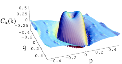
Figure 11: Correlation of the standard map in the near-integrable regime. The parameters are $N=500$ and $k=0.5$.

V Discussion

We have derived semiclassical expressions of the correlation of level velocities and overlap intensities in near-integrable systems. Their $\hbar$-scaling is very different than previously derived in the chaotic limit cerruti:01 where the level velocity variance is

$$\sigma^{2}_{E}\propto\hbar^{d-1}$$ (47)

and the intensity variance note is

$$\sigma^{2}_{\alpha}\propto\hbar^{2d-1}$$ (48)

In addition, for chaotic systems the action derivatives will eventually decouple from the weightings in the correlation so that in the semiclassical limit the random matrix theory prediction is recovered stating that no correlations exist tomsovic:96 ; cerruti:01 . On the other hand, for finite $\hbar$ with the average computed up to the Heisenberg time, there is a possibility of short orbits that do not decouple in chaotic systems, so correlations may exist. For near-integrable systems there is no decoupling even in the long time limit.

Combining the previously derived results in chaotic systems with the newly derived results for near-integrable systems, for mixed phase space systems we attempted to separate the orbits for applying the Hannay-Ozorio de Almeida sum rule to the different regions of phase space. Several criteria were chosen as a basis for the separation. All of them led to inconsistencies in the interpretation. It seems that all of the unstable orbits spend some part of their evolution mimicking stable motion and do not give standard diffusion contributions to action derivatives. Nevertheless, a different semiclassical procedure lakshminarayan:99 , not going through the Hannay-Ozorio sum rule derivation, gives a theoretical prediction that matches well with the level velocity variances independently of the dynamical regime of the system.

Finally, the correlation between the level velocities and the intensities has been shown to highlight resonance zones in near-integrable systems. The resonance zones exhibit greater localization since the motion is bounded within the separatrix. Investigating the correlation and covariance separably may yield more information about the system. An example is the dip in the correlation that occurs near the center of the resonance zone due to the stable periodic orbit; the dip is not present in the covariance.

Appendix A Level Velocities

The method berry:94 to obtain the variance of the level velocities begins with the smoothed spectral staircase

$$N_{\epsilon}(E,\lambda)=\sum_{n}\theta(E-E_{n}(\lambda))$$ (49)

Taking the derivative with respect to the parameter, we obtain

$${\partial N_{\epsilon}(E,\lambda)\over\partial\lambda}=\sum_{n}\delta(E-E_{n}(\lambda)){\partial E_{n}(\lambda)\over\partial\lambda}$$ (50)

The quantity $\epsilon$ is an energy smoothing term which will be taken smaller than the mean level spacing. Upon energy averaging

$$\left\langle{\partial N_{\epsilon}(E,\lambda)\over\partial\lambda}\right\rangle_{E}=\overline{d}(E,\lambda)\left\langle{\partial E_{n}(\lambda)\over\partial\lambda}\right\rangle_{n}$$ (51)

where $\overline{d}(E,\lambda)$ is the mean level density which is the reciprocal of the mean level spacing and proportional to $\hbar^{-d}$. The mean level spacing is related to the phase space volume by $V=\overline{d}\hbar^{d}$. Thus, in order to obtain information about the level velocities, we will evaluate the spectral staircase.

The semiclassical construction of the spectral staircase is broken into an average and an oscillating part

$$N_{\epsilon}(E,\lambda)=\overline{N}(E,\lambda)+N_{osc}(E,\lambda)$$ (52)

The average staircase $\overline{N}(E,\lambda)$ is the Weyl term and to leading order in $\hbar$ is given by

$$\overline{N}(E,\lambda)={1\over h^{d}}\int\theta(E-H({\bf I},{\bm{\theta}};\lambda)d{\bf I}d{\bm{\theta}}$$ (53)

The oscillating part of the spectral staircase is a sum over rational tori with topology ${\bf M}$ of the unperturbed Hamiltonian, $H_{0}({\bf I})$ ullmo:96

$$N_{osc}(E,\lambda) = {2\over\hbar^{(d-1)/2}}\sum_{\bf M}{}^{\prime}A_{\bf M}$$ (54)

$$\times\mathrm{Re}\left\{\exp\left({i\overline{S}_{\bf M}(\lambda)\over\hbar}-{i\eta_{\bf M}\pi\over 2}+{i\beta_{\bf M}\pi\over 4}\right)\right.$$

$$\times[J_{0}(\Delta S_{\bf M}(\lambda)/\hbar)-i\tilde{a}(\lambda)J_{1}(\Delta S_{\bf M}(\lambda)/\hbar)]$$

$$\times\left.\exp\left({-\epsilon T_{\bf M}\over\hbar}\right)\right\}$$

The phase $\eta_{\bf M}={\bf M}\cdot{\bm{\eta}}$ where ${\bm{\eta}}$ are the Maslov indices and $\beta_{\bf M}$ is equal to the sign of the determinant of the curvature matrix.

The variance of the level velocities is obtained by taking the mean square of the counting function derivatives

$$\left\langle\left({\partial N_{\epsilon}(E,\lambda)\over\partial\lambda}\right)^{2}\right\rangle_{E}=\left\langle\sum_{n}\sum_{m}{\partial E_{n}(\lambda)\over\partial\lambda}{\partial E_{m}(\lambda)\over\partial\lambda}\right.$$

$$\times\left.\delta_{\epsilon}(E-E_{n}(\lambda))\delta_{\epsilon}(E-E_{m}(\lambda))\frac{}{}\right\rangle_{E}$$ (55)

For a nondegenerate spectrum, the summation is nonzero only if $n=m$ because of the product of the two delta functions. Since Lorentzian smoothing is applied, then

$$\delta^{2}_{\epsilon}(x)={1\over 2\pi\epsilon}\delta_{\epsilon/2}(x)$$ (56)

for $\epsilon\ll\overline{d}^{-1}$. Thus we have

$$\left\langle\left({\partial N_{\epsilon}(E,\lambda)\over\partial\lambda}\right)^{2}\right\rangle_{E}={\overline{d}\over 2\pi\epsilon}\left\langle\left({\partial E_{n}(\lambda)\over\partial\lambda}\right)^{2}\right\rangle_{n}$$ (57)

The summation over the rational tori is most sensitive to the changing actions and periods because of the associated rapidly oscillating phases, i.e., the division by $\hbar$ in the exponential. Since the energy smoothing term $\epsilon$ is taken smaller than a mean level spacing, it scales at least by $\hbar^{d}$ and the derivatives of the period vanish as $\hbar\rightarrow 0$. Thus, only the derivatives of the actions are considered, and the oscillating part of the staircase yields

$${\partial N_{osc}(E)\over\partial\lambda}\approx{2\over\hbar^{(d+1)/2}}\sum_{\bf M}{}^{\prime}A_{\bf M}\mathrm{Im}\left\{-\exp\left({i\overline{S}_{\bf M}(\lambda)\over\hbar}-{i\eta_{\bf M}\pi\over 2}+{i\beta_{\bf M}\pi\over 4}\right)\right.$$

$$\times\left.\left[\left(\partial\overline{S}_{\bf M}\over\partial\lambda\right)[J_{0}(s_{\lambda})-i\tilde{a}(\lambda)J_{1}(s_{\lambda})]+i\left(\partial\Delta S_{\bf M}\over\partial\lambda\right)\left(J_{1}(s_{\lambda})+{i\tilde{a}(\lambda)\over 2}[J_{0}(s_{\lambda})-J_{2}(s_{\lambda})]\right)\right]\exp\left({-\epsilon T_{\bf M}\over\hbar}\right)\right\}$$ (58)

After making the diagonal approximation and energy averaging, the variance of the level velocities for a near-integrable system is

$$\sigma^{2}_{E} \approx {4\pi\epsilon\over V\hbar}\sum_{\bf M}{}^{\prime}\left\langle A_{\bf M}^{2}\left\{\left(\partial\overline{S}_{\bf M}\over\partial\lambda\right)^{2}[J_{0}^{2}(s_{\lambda})+\tilde{a}^{2}J_{1}^{2}(s_{\lambda})]\right.\right.+2\left(\partial\overline{S}_{\bf M}\over\partial\lambda\right)\left(\partial\Delta S_{\bf M}\over\partial\lambda\right)\left[{\tilde{a}\over 2}J_{0}(s_{\lambda})(J_{0}(s_{\lambda})-J_{2}(s_{\lambda}))+\tilde{a}J_{1}^{2}(s_{\lambda})\right]$$ (59)

$$+\left.\left.\left(\partial\Delta S_{\bf M}\over\partial\lambda\right)^{2}\left[{\tilde{a}^{2}\over 4}(J_{0}(s_{\lambda})-J_{2}(s_{\lambda}))^{2}+J_{1}^{2}(s_{\lambda})\right]\right\}\exp\left({-2\epsilon T_{\bf M}\over\hbar}\right)\right\rangle_{E}$$

The middle term vanishes since $(\partial\overline{S}_{\bf M}/\partial\lambda)$ and $(\partial\Delta S_{\bf M}/\partial\lambda)$ are uncorrelated and both average to zero.

Appendix B Overlap Intensities

The variance of the intensities is derived by examining the oscillating part of the strength function

$$S_{\alpha,osc}(E,\lambda)={-1\over\pi}\mathrm{Im}\int\langle\alpha|{\bm{\theta}}\rangle G({\bm{\theta}},{\bm{\theta}}^{\prime};E)\langle{\bm{\theta}}^{\prime}|\alpha\rangle d{\bm{\theta}}d{\bm{\theta}}^{\prime}$$ (60)

where

$$G({\bm{\theta}},{\bm{\theta}}^{\prime};E) = {1\over i\hbar(2\pi i\hbar)^{(d-1)/2}}\sum_{j}|D_{s}|^{1/2}$$ (61)

$$\times\exp[iS_{j}({\bm{\theta}},{\bm{\theta}}^{\prime};E)/\hbar-i\nu_{j}^{\prime}\pi/2]$$

is the semiclassical energy Green’s function. The above sum is over all paths that connect ${\bm{\theta}}$ to ${\bm{\theta}}^{\prime}$ on a given energy surface $E$. $D_{s}$ is a determinate involving second derivatives of the actions

$$D_{s}=\left|\begin{array}[]{cc}{\partial^{2}S\over\partial{\bm{\theta}}\partial{\bm{\theta}}^{\prime}}&{\partial^{2}S\over\partial{\bm{\theta}}\partial E}\\ {\partial^{2}S\over\partial E\partial{\bm{\theta}}^{\prime}}&{\partial^{2}S\over\partial E^{2}}\\ \end{array}\right|$$ (62)

We assume that the Gaussian wave packet in Cartesian coordinates can be define locally as a Gaussian in action-angle variables using the Wigner function

$$A_{W}({\bf I},{\bm{\theta}})=2^{d}\exp\{-(\Delta{\bf I})^{2}/\hbar^{2}-(\Delta{\bm{\theta}})^{2}\}$$ (63)

where $(\Delta{\bf I})_{j}\equiv\sigma_{j}({\bf I}-{\bf I}_{\alpha})_{j}$ and $(\Delta{\bm{\theta}})_{j}\equiv({\bm{\theta}}-{\bm{\theta}}_{\alpha})_{j}/\sigma_{j}$. The inverse transform is evaluated by stationary phase to obtain

$$\langle\alpha|{\bm{\theta}}\rangle\langle{\bm{\theta}}^{\prime}|\alpha\rangle={1\over\pi^{d/2}\prod\sigma_{j}}$$ (64)

$$\times\exp\left[{-(\Delta{\bm{\theta}})^{2}\over 2}-{(\Delta{\bm{\theta}^{\prime}})^{2}\over 2}+{i({\bf I}-{\bf I}_{\alpha})\cdot({\bm{\theta}}-{\bm{\theta}}^{\prime})\over\hbar}\right]$$

The Gaussian localization in action-angle space implies that the dominant contributions to the strength function arise from tori whose trajectories are closed, i.e., rational tori ${\bf I_{M}}$. An expansion about the center of the Gaussian wave packet yields

$$S_{j}({\bm{\theta}},{\bm{\theta}}^{\prime};E)=S_{\bf M}({\bm{\theta}}_{\alpha},{\bm{\theta}}_{\alpha};E)+{\bf I}_{j}\cdot({\bm{\theta}}-{\bm{\theta}}^{\prime})$$ (65)

where quadratic terms have been neglected. Using the above expansion of the action, the integrals over the angles can be performed by stationary phase giving

$$S_{\alpha,osc}(E,\lambda) \approx {2^{(d+1)/2}\prod\sigma_{j}\over\pi^{1/2}\hbar^{(d+1)/2}}\sum_{\bf M}{}^{\prime}|D_{s}|^{1/2}$$

$$\times \cos\left({S_{\bf M}\over\hbar}-{\eta_{\bf M}\pi\over 2}+{\beta_{\bf M}\pi\over 4}\right)\exp\left[{-(\Delta{\bf I})^{2}\over\hbar^{2}}\right]$$

The above result for the oscillatory part of the strength function can be used to obtain the variance of intensities as

$$\sigma^{2}_{\alpha} = {2\pi\epsilon\over\overline{d}}\left\langle S^{2}_{\alpha,osc}(E,\lambda)\right\rangle_{E}$$ (67)

$$\approx {\epsilon 2^{d+1}\prod\sigma^{2}_{j}\over V\hbar}\left\langle\sum_{\bf M}{}^{\prime}|D_{s}|\exp\left[{-2(\Delta{\bf I})^{2}\over\hbar^{2}}\right]\right.$$

$$\times\left.\exp\left({-2\epsilon T_{\bf M}\over\hbar}\right)\right\rangle_{E}$$

where we have used the diagonal approximation for the sum over ${\bf M}$. Since the trace of the Green function is the density of states given by Berry and Tabor and the density of states is the energy derivative of the spectral staircase function, then $|D_{s}|=T^{2}_{\bf M}A^{2}_{\bf M}/(2\pi)^{d-1}$. Hence, given the Hannay-Ozorio sum rule for $\sum_{\bf M}A^{2}_{\bf M}$, Eq. (9), then

$$\sum_{\bf M}{}^{\prime}|D_{s}|\cdots\rightarrow{V\over(2\pi)^{d}}\int dT\cdots$$ (68)

Since the Gaussian weighting of the action variables is independent of the period, it follows that

$$\sigma^{2}_{\alpha}\approx{\prod\sigma^{2}_{j}\over\pi^{d}}\left\langle\exp\left[{-2(\Delta{\bf I})^{2}\over\hbar^{2}}\right]\right\rangle_{\bf M}$$ (69)

Appendix C Ballistic Vs. Diffusive Behavior

We tried three different methods for separating out the ballistic and diffusive orbits. The fraction of ballistic orbits $f$ was deduced by

$$f={c_{2}(k)\over 4\pi^{2}\zeta(k)}$$ (70)

where $c_{2}(k)$ was determined by Eq. (44). The first method was to divide the orbits by a fixed value of the Lyapunov exponent. It turned out that a Lyapunov exponent of 0.5 gave fairly good result, but there is no explanation of this value. Table 1 summarizes these results.

Table 1: Fixed Lyapunov exponent cutoff. $f_{1}$ is the fraction of orbits that have a Lyapunov exponent less than $\mu=0.5$.

$k$	$\zeta(k)$	$f$	$f_{1}$
1.5	$9.62\times 10^{-5}$	0.982	1.000
2.0	$1.11\times 10^{-4}$	0.856	0.798
2.5	$1.76\times 10^{-4}$	0.358	0.336
3.0	$3.66\times 10^{-4}$	0.161	0.142
3.5	$3.58\times 10^{-4}$	0.166	0.146
4.0	$3.67\times 10^{-4}$	0.118	0.107

The next method was to take twice the fraction of stable orbits as the number of ballistic orbits. This is summarized in Table 2.

Table 2: Twice the regular orbits. $f_{2}$ is twice the fraction of regular orbits and $\mu_{2}$ is the cutoff of the Lyapunov exponent associated with $f_{2}$.

$k$	$\zeta(k)$	$f$	$f_{2}$	$\mu_{2}$
1.5	$1.17\times 10^{-4}$	0.812	0.687	0.318
2.0	$1.49\times 10^{-4}$	0.638	0.526	0.443
2.5	$2.19\times 10^{-4}$	0.288	0.256	0.420
3.0	$2.19\times 10^{-4}$	0.269	0.241	0.590
3.5	$2.21\times 10^{-4}$	0.268	0.246	0.702
4.0	$2.29\times 10^{-4}$	0.189	0.179	0.713

For the final method we took the greatest number of orbits up to some Lyapunov exponent that did not change $\zeta(k)$ significantly as the number of ballistic orbits and is summarize is Table 3.

Table 3: Stable quadratic. $f_{3}$ is the number of orbits included in the ballistic term which does not change its coefficient significantly. $\mu_{3}$ is the corresponding Lyapunov exponent.

$k$	$\zeta(k)$	$f$	$f_{3}$	$\mu_{3}$
1.5	$1.84\times 10^{-4}$	0.516	0.412	0.2
2.0	$2.58\times 10^{-4}$	0.368	0.302	0.3
2.5	$3.30\times 10^{-4}$	0.191	0.165	0.2
3.0	$4.26\times 10^{-4}$	0.139	0.124	0.4
3.5	$4.01\times 10^{-4}$	0.148	0.137	0.4
4.0	$4.31\times 10^{-4}$	0.105	0.100	0.4

References

- (1) H. U. Baranger and P. A. Mello, Phys. Rev. Lett. 73, 142 (1994); A. M. Chang, H. U. Baranger, L. N. Pfeiffer, K. W. West and T. Y. Chang, Phys. Rev. Lett 76, 1695 (1996); J. A. Folk, S. R. Patel, S. F. Godijn, A. G. Huibers, S. M. Cronenwett, C. M. Marcus, K. Campman and A. C. Gossard, Phys. Rev. Lett 76, 1699 (1996); C. W. J. Beenakker, Rev. Mod. Phys. 69, 731 (1997)
- (2) S. Sridhar and A. Kudrolli, Phys. Rev. Lett. 72, 2175 (1994).
- (3) K. Schaadt and A. Kudrolli, Phys. Rev. E 60, R3479 (1999).
- (4) For a recent review see M. Gruebele, Adv. Chem. Phys. 114, 193 (2000).
- (5) G. T. Fraser and B. H. Pate, J. Chem. Phys. 100, 6210 (1994); J. Ortigoso, G. T. Fraser, and B. H. Pate, Phys. Rev. Lett. 82, 2856 (1999).
- (6) B. D. Simons, P. A. Lee and B. L. Altshuler, Phys. Rev. Lett. 70, 4122 (1993).
- (7) M. V. Berry, J. Phys. A 10, 2083 (1977); A. Voros, in Stochastic Behavior in Classical and Quantum Hamiltonian Systems, edited by G. Casati and G. Ford, Lecture Notes in Physics No. 93 (Springer, Berlin, 1979), p. 326.
- (8) K. Takahashi, J. Phys. Soc. Jpn. 55, 762 (1986).
- (9) J. Kurchan, P. Leboeuf and M. Saraceno, Phys. Rev. A 40, 6800 (1989).
- (10) J. H. Hannay and A. M. Ozorio de Almeida, J. Phys. A: Math. Gen. 17, 3429 (1984).
- (11) S. Tomsovic, Phys. Rev. Lett. 77, 4158 (1996).
- (12) N. R. Cerruti and S. Tomsovic, in preparation.
- (13) S. Keshavamurthy, N. R. Cerruti and S. Tomsovic, J. Chem. Phys. 117, 4168 (2002).
- (14) Y. Weissman and J. Jortner, J. Chem. Phys. 77, 1469 (1982); 1486 (1982).
- (15) D. Ullmo, M. Grinberg, and S. Tomsovic, Phys. Rev. E 54, 136 (1996).
- (16) M. V. Berry and M. J. Tabor, Phys. A: Math. Gen. 10, 371 (1977).
- (17) M. V. Berry and J. P. Keating, J. Phys. A 27, 6167 (1994).
- (18) P. Leboeuf and M. Sieber, Phys. Rev. E 60, 3969 (1999).
- (19) N. R. Cerruti, A. Lakshminarayan, J. H. Lefebvre and S. Tomsovic, Phys. Rev. E 63, 016208 (2001); A. Lakshminarayan, N. R. Cerruti and S. Tomsovic, Phys. Rev. E 63, 016209 (2001).
- (20) A. M. Ozorio de Almeida in Quantum Chaos and Statistical Nuclear Physics, edited by T. H. Seligman and H. Nishioka, Lecture Notes in Physics 263 (Springer, Berlin, 1986).
- (21) G. Casati, B. V. Chirikov, and I. Guarneri, Phys. Rev. Lett. 54, 1350 (1985); M. V. Berry, Proc. R. Soc. Lond. A 400, 229 (1985).
- (22) A. Lakshminarayan, Pramana 48, 517 (1997).
- (23) P. W. O’Connor and S. Tomsovic, Ann. Phys. (NY) 207, 218 (1991); A. M. Ozorio de Almeida and M. Saraceno, Ann. Phys. (NY) 210, 1 (1991).
- (24) A. Lakshminarayan, N. R. Cerruti and S. Tomsovic, Phys. Rev. E 60, 3992 (1999).
- (25) P. Grassberger, R. Badii and A. Politi, J. Stat. Phys. 51, 135 (1988).
- (26) T. Dittrich and U. Smilansky, Nonlinearity 4, 59 (1991).
- (27) This scaling of the variance of the intensities differs from our previous publication (Ref. cerruti:01 ), which contained an error in the derivation of the average intensities and sum rule.