Stable solitons in coupled Ginzburg-Landau equations describing Bose-Einstein condensates and nonlinear optical waveguides and cavities

We introduce a model of a two-core system, based on an equation of the Ginzburg-Landau (GL) type, coupled to another GL equation, which may be linear or nonlinear. One core is active, featuring intrinsic linear gain, while the other one is lossy. The difference from previously studied models involving a pair of linearly coupled active and passive cores is that the stabilization of the system is provided not by a linear diffusion-like term, but rather by a cubic or quintic dissipative term in the active core. Physical realizations of the models include systems from nonlinear optics (semiconductor waveguides or optical cavities), and a double-cigar-shaped Bose-Einstein condensate with a negative scattering length, in which the active “cigar” is an atom laser. The replacement of the diffusion term by the nonlinear loss is principally important, as diffusion does not occur in these physical media, while nonlinear loss is possible. A stability region for solitary pulses is found in the system’s parameter space by means of direct simulations. One border of the region is also found in an analytical form by means of a perturbation theory. Moving pulses are studied too. It is concluded that collisions between them are completely elastic, provided that the relative velocity is not too small. The pulses withstand multiple tunneling through potential barriers. Robust quantum-rachet regimes of motion of the pulse in a time-periodic asymmetric potential are found as well.

PACS number: 42.81.Dp, 03.75.Lm, 42.65.Tg

1 Introduction

Ginzburg-Landau (GL) equations represent a class of universal mathematical models which describe pattern formation in various nonlinear media [1]. One of the most fundamental types of patterns are solitary pulses (SPs), in loose terms often called solitons. In particular, the simplest generic species of the GL equations, viz., the cubic complex one, gives rise to a well-known exact SP solution [2]. However, this solution is unstable (as the equation includes a linear gain term, which makes the zero solution unstable, precluding stability of any solitary pattern). Therefore, search for physically relevant models of the GL type that give rise to stable pulses has attracted much attention. One possibility is to introduce a cubic-quintic GL equation with linear loss and cubic gain, nonlinear stability being provided by a quintic loss term. Stable SPs in equations of the latter type have been studied in detail [3]. Another model, which finds a straightforward physical realization in terms of dual-core nonlinear optical fibers, was proposed in Ref. [4]. In this system, one core carries linear gain, while the other one is lossy, the corresponding model being based on a system of two linearly coupled cubic GL equations (in fact, the one corresponding to the lossy core may be a linear equation).

Detailed investigations have demonstrated that the latter model supports stable stationary SPs [5, 6] and their bound states [7] in broad parametric regions. Stable moving pulses, randomly wandering ones, and breathers (both standing and moving) have also been found in this system [8]. The model was subsequently generalized to combine it with dispersion-management [9] and wavelength-division-multiplexing (i.e., multi-channel) [10] schemes, which opens a way for applications to fiber-optic telecommunications. It was also shown that a model of the same type can support stable dark solitons [11].

In all the cases, the stability of SP solutions in this model was provided by a linear dispersive-loss term, which accounted for the bandwidth-limited character of the gain in the active core (formally, that term is tantamount to diffusion). Without this ingredient, the model can generate only unstable SPs. However, the natural bandwidth of the optical gain (which is usually provided for by the Erbium dopant [12]) is very broad, therefore the limitation of the gain bandwidth should be enforced by optical filters specially inserted into the system. A related problem is that, in the case of other physical systems which may be described by equations of the GL types, such as optical cavities or planar waveguides and Bose-Einstein condensates (BECs, see below), the diffusion term is not physically possible at all.

An alternative way to stabilize SPs is to use a nonlinear dissipative term, which may be cubic or quintic. In the applications to nonlinear optics, a cubic loss term is naturally generated by two-photon absorption, which is a strong effect in semiconductor waveguides and semiconductor-doped glasses (see, e.g., recent works [13] and [14], respectively, and references therein). The investigation of this possibility is a subject of the present work. Actually, the system with nonlinear loss and without filtering/diffusion is not just another version of the above-mentioned dual-core fiber-optic model, but it also directly applies to the description of other physical media, namely, nonlinear optical cavities and BECs, as it is explained below.

In normalized units, coupled equations of the type described above can be cast in the form

$$u_{t} = \gamma u+i\gamma_{2}u_{xx}+\left(i\sigma_{1}-\sigma_{2}\right)|u|^{2}u+iv,$$ (1)

$$v_{t} = -\left(\Gamma+i\chi\right)v+i\gamma_{2}v_{xx}+iu,$$ (2)

where, in the case of the optical systems, $u$ and $v$ are amplitudes of electromagnetic waves in two cores of the system, the evolutional variable $t$ is either time or propagation distance in the optical cavity (depending on the physical formulation [15]), or the propagation distance in the dual-core optical fiber, and $x$ is the transverse coordinate in the cavity (or in a planar waveguide), or the reduced time in the application to the fibers. Further, the term with $\gamma>0$ in Eq. (1) accounts for the gain in the active subsystem, the constant of linear coupling between the cores is normalized to be $1$, $\Gamma>0$ is the dissipative constant in the lossy subsystem, $\chi$ is a possible frequency- (if $t$ is time) or wavenumber- (if $t$ is the propagation distance) mismatch between the cores, and $\gamma_{2}$, which may be assumed positive, is the dispersion/diffraction coefficient (in fact, $\gamma_{2}$ may be given a fixed value by means of obvious rescaling; $\gamma_{2}=5$ will be chosen below, as this value is convenient to display numerical results). Finally, $\sigma_{2}$ and $\sigma_{1}$ are, respectively, coefficients of the Kerr nonlinearity and nonlinear loss in the active core. It is assumed that, in most cases, the field in the lossy core is much weaker than in the active one, therefore nonlinear terms in Eq. (2) may be neglected [6, 8], although properties of SPs in the system including nonlinear terms in the lossy subsystem are quite similar to those in the system based on Eqs. (1) and (2) [5, 6]. A principal difference of the model based on Eqs. (1) and (2) from the previously considered ones is that the coefficient in front of the term $iu_{xx}$ in Eqs. (1) and (2) is real, while the nonlinear coefficient in Eq. (1) is complex; previously, exactly the opposite case was considered [5, 6, 8].

In the application to BECs, each equation (1) and (2) may be realized as a one-dimensional Gross-Pitaevskii equation for a condensate in a cigar-shaped trap, with the linear coupling induced by tunneling between them (see, e.g., Ref. [16]). The second derivatives in Eqs. (1) and (2) are then the kinetic-energy terms, with $\gamma_{2}=\hbar/2m$, where $m$ is the atomic mass. The linear-loss term in Eq. (2) accounts for evaporation of condensate atoms in the second trap, while the linear gain in Eq. (1) assumes that the corresponding trap is arranged as an atom-wave laser [17]. Further, the coefficient $\sigma_{1}$ in Eq. (1) is proportional to the scattering length of atomic collisions in the BEC gas, and $\sigma_{2}>0$ accounts for effective loss due to two-body collisions [18].

In fact, in many cases a dominant contribution to the nonlinear loss in BECs is due to three-body collisions [19], hence the corresponding dissipative term is quintic, and the accordingly modified equation (1) takes the form (again, with $\sigma_{2}>0$)

$$u_{t}=\gamma u+i\gamma_{2}u_{xx}+\left(i\sigma_{1}-\sigma_{2}|u|^{2}\right)|u|^{2}u+iv.$$ (3)

Below, we will consider two systems, (1), (2) and (3), (2) with the cubic and quintic nonlinear-loss terms, respectively.

The rest of the paper is organized as follows. In Section 2 we present analytical results for SPs obtained by means of a perturbation theory. Numerical results are displayed in Section 3, where a parametric region for the existence of stable SPs is identified. In Section 4, we consider moving solitons, demonstrating that they collide elastically with each other. We also consider a generalization of the model including an $x$-dependent potential, which is relevant for BECs, and may be relevant for the case of optical planar waveguides too. In that case, we find that moving SPs can coherently tunnel (many times) through a potential barrier. The paper is concluded by Section 5.

2 Analytical results

Following the lines of Ref. [4], it is possible to develop analysis of SP solutions, considering them as weakly perturbed nonlinear Schrödinger (NLS) solitons. The linear coupling between the two equations, as well as the gain and loss terms, are treated as perturbations, which are ordered so that the conservative one, i.e., the linear coupling, is assumed to be a larger perturbation, while the nonconservative terms are assumed to be a smaller perturbation. Thus, in the lowest-order approximation, that ignores the loss and gain but takes the coupling into regard at the first order of the perturbation theory, the SP has the form

$$u=\frac{\eta}{\sqrt{\sigma_{1}}}\,\mathrm{sech}\left(\frac{\eta\,x}{\sqrt{2\gamma_{2}}}\right)\exp\left(\frac{i}{2}\eta^{2}t\right),\,v=V(x)\exp\left(\frac{i}{2}\eta^{2}t\right),$$ (4)

where it is assumed that $\sigma_{1}$ is positive, $\eta$ is an arbitrary real constant, which is an intrinsic parameter of the soliton family, and the real function $V(x)$ is a solution to the linear inhomogeneous equation,

$$\gamma_{2}\frac{d^{2}V}{dx^{2}}-\left(\frac{1}{2}\eta^{2}+\chi\right)V=-\frac{\eta}{\sqrt{\sigma_{1}}}\,\mathrm{sech}\left(\frac{\eta\,x}{\sqrt{2\gamma_{2}}}\right).$$ (5)

Note that, in this approximation, the linearly coupled equations conserve three dynamical invariants: the Hamiltonian and momentum, expressions for which will not be used here, and the norm $N$, which has the physical meaning of energy or power in the applications to optics (depending on the particular interpretation – it is energy in the fiber, or power in the cavity or planar waveguide), or the total number of atoms in the case of BECs,

$$N=\int_{-\infty}^{+\infty}\left[\left|u(x)\right|^{2}+\left|v(x)\right|^{2}\right]dx.$$ (6)

In the next approximation, when the nonconservative perturbations are taken into account, we assume that $\eta$ may be a slowly varying function of time [then, the expression $(1/2)\eta^{2}t$ for the SP phase in Eq. (4) is replaced by $(1/2)\int\eta^{2}(t)dt$]. An evolution equation for $\eta(t)$ can be derived from the balance equation for $N$ . In the case of the cubic loss term, which corresponds to Eq. (1), it is

$$\frac{dN}{dt}=2\int_{-\infty}^{+\infty}\left[\gamma\left|u(x)\right|^{2}-\Gamma\left|v(x)\right|^{2}\right]dx-2\sigma_{2}\int_{-\infty}^{+\infty}\left|u(x)\right|^{4}dx.$$ (7)

In the case of the quintic loss term, corresponding to Eq. (3), $\left|u(x)\right|^{4}$ in the last term of Eq. (7) is replaced by $\left|u(x)\right|^{6}$.

By itself, Eq. (7) is an exact one. To derive the evolution equation for $\eta(t)$ from it, we substitute the approximation (4) for $u$, and make use of Eq. (5) (which is solved by means of the Fourier transform). Then, after straightforward calculations following the pattern of Ref. [4], the resultant evolution equation can be obtained in an explicit form if $\chi=0$. With the cubic loss term, it takes the form

$$\frac{d\eta}{dt}=2\gamma\eta-\frac{4\sigma_{2}}{3\sigma_{1}}\eta^{3}-C\Gamma\eta^{-3},$$ (8)

where $C\equiv\left(\pi^{2}/6\right)+\zeta(3)\approx 2.845$, and $\zeta$ is the Riemann’s zeta-function. If the loss term is quintic, Eq. (8) is replaced by

$$\frac{d\eta}{dt}=2\gamma\eta-\frac{16\sigma_{2}}{15\sigma_{1}}\eta^{5}-C\Gamma\eta^{-3}.$$ (9)

Stationary SP solutions are selected from the continuous soliton family as fixed points (FPs) of Eq. (8) or (9), i.e., as roots of the expression on the right-hand side of the equation. The roots can be found in a simple form in the case of Eq. (9):

$$\eta_{\mathrm{FP}}^{4}=\left(16\sigma_{2}\right)^{-1}\left[15\sigma_{1}^{2}\gamma\pm\sqrt{15\sigma_{1}^{2}\left(15\sigma_{1}^{2}\gamma^{2}-16C\sigma_{2}\Gamma\right)}\right].$$ (10)

An elementary consideration demonstrates that, in either model, there may exist two physical FPs or none, depending on values of the parameters: in the case of Eq. (8), physical solutions exist if

$$2\sigma_{1}^{2}\gamma^{3}\geq 3C\sigma_{2}^{2}\Gamma,$$ (11)

and in the case of Eq. (9), this condition is replaced by [as it immediately follows from Eq. (10)]

$$15\sigma_{1}^{2}\gamma^{2}\geq 16C\sigma_{2}\Gamma;$$ (12)

note that $\gamma_{2}$ does not appear in Eqs. (11) and (12). Further, it follows from Eqs. (8) and (9) that the FP corresponding to a smaller value of $\eta$ [for instance, the one with the lower sign in Eq. (10)] is unstable, while the FP corresponding to larger $\eta$ is stable (within the framework of the present approximation). In the next section, these analytical predictions will be compared with results of direct numerical simulations.

Lastly, we notice that the stability of the zero solution is a necessary condition for the full stability of any solitary pattern. In turn, simple necessary (but, generally speaking, not sufficient) conditions for the zero-solution stability take a simple form in the case $\chi=0$ [4]: $\gamma<\Gamma<1/\gamma$ (which implies that $\gamma$ must be smaller than $1$).

3 Numerical results

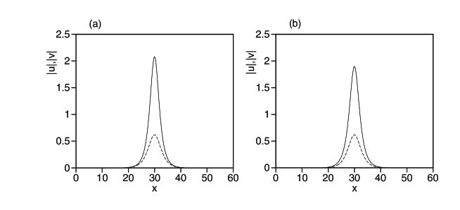
Figure 1: Examples of stable stationary solitary-pulse solutions to (a) Eqs. (1), (2), and (b) Eqs. (3), (2), found for (a) $\gamma=0.4,\sigma_{1}=1,\sigma_{2}=0.1,\gamma_{2}=5,\Gamma=1,\chi=0$, and (b) $\gamma=0.5,\Gamma=1,\gamma_{2}=5,\sigma_{1}=1,\sigma_{2}=0.05,\chi=0$. The continuous and dashed curves show $|u(x)|$ and $|v(x)|$, respectively.

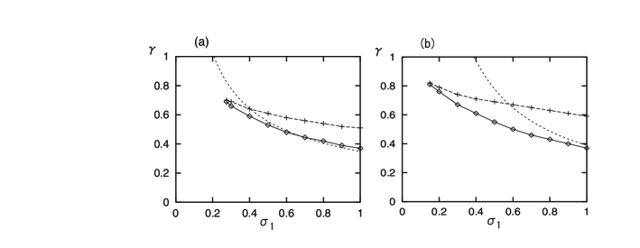
Figure 2: A generic example of the stability region for solitary pulses in the model (1), (2) (a) and (3), (2) (b), as found in a numerical form. The fixed parameters are $\sigma_{2}=0.1,\gamma_{2}=5,\Gamma=1,\chi=0$ in (a), and $\sigma_{2}=0.05,\gamma_{2}=5,\Gamma=1,\chi=0$ in (b). The curve denoted by crosses is a border above which some perturbations with high wavenumbers grow and SPs are destroyed. The curve denoted by diamonds is a border below which SPs decays to zero. The dashed curve in each panel is the existence border for the pulses predicted in the analytical form by (a) Eq. (11) or (b) Eq. (12).

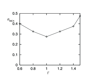
Figure 3: The minimum value of the nonlinear coefficient $\sigma_{1}$, up to which stable solitary pulses were found in Eqs. (1), (2), varying the gain $\gamma$, as a function of the linear-loss coefficient $\Gamma$. The other coefficients were fixed: $\sigma_{2}=0.1,\;\gamma_{2}=5$, and $\chi=0$.

Figure 4: A typical example of multiple collisions between two moving solitons in Eqs. (1) and (2) with periodic boundary conditions. The parameters are $\sigma_{2}=0.1,\gamma_{2}=5,\Gamma=1,\chi=0$ and the spatial period is $L=60$. The initial wavenumbers of the pulses [see Eqs. (1) and (2)] are $k=\pm 0.5$.

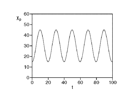
Figure 5: Time evolution of the peak position of the oscillating pulse in the harmonic potential $U(x)=(K/2)(x-L/2)^{2}$ with $K=0.01$ for $\gamma=0.4,\;\sigma_{2}=0.1,\;\hbar=1,\;m=0.1,\Gamma=1,\chi=0$.

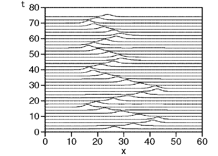
Figure 6: An example of multiple coherent tunneling of a traveling solitary pulse across a narrow potential barrier (19) in the model (17), (18). The parameters are $\gamma=0.4,\;\sigma_{2}=0.1,\;\hbar=1,\;m=0.1,\Gamma=1,\;\chi=0$, and the initial wavenumber pushing the pulse is $k=0.4$.

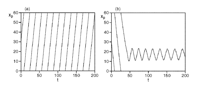
Figure 7: An example of the quantum-ratchet effect for traveling pulses in the time-periodic sawtooth potential (20) for $\gamma=0.4,\;\sigma_{2}=0.1,\;\hbar=1,\;m=0.1,\Gamma=1,\chi=0$. The initial velocity is $4$ in (a) and $-4$ in (b). The temporal dependences of the peak position $X_{p}$ are displayed in both panels.

In the numerical investigation, SP solutions were looked for as solutions to the stationary version of Eqs. (1), (2) or (3), (2); then, stability of the obtained solutions was tested in simulations of the full time-dependent equations. Typical examples of thus found stable SPs in both models are displayed in Fig. 1.

Results of systematic numerical simulations of Eqs. (1), (2) and (3), (2) are summarized in Fig. 2, which displays generic examples of stability regions for SPs in the parameter plane $\left(\sigma_{1},\gamma\right)$. These two parameters are chosen for the variation, while the others are fixed, as they can be readily varied in the experimental studies of BECs: the gain $\gamma$ is controlled by intrinsic parameters of the atom laser, and the nonlinearity $\sigma_{1}$ can be changed by means of the Feshbach resonance [20]. In the applications to optics, the gain parameter is also easy to vary.

The analytical predictions (11) and (12) for the existence of SPs correlate with lower borders of the numerically found stability regions in Figs. 2(a) and 2(b). As is seen, the perturbative result is accurate enough for relatively large values of $\sigma_{1}$ and small values of $\gamma$, when the gain and loss may indeed be regarded as small perturbations; with the decrease of $\sigma_{1}$ and increase of $\gamma$, the perturbations are no longer small, which explains discrepancy between the analytically predicted and numerically found lower borders in Figs. 2(a) and 2(b) in this case.

Below the existence border, the perturbation theory predicts that no stationary SP exists; in accord with this, the numerical simulations show that, beneath the lower border, any initial pulse decays to zero. On the other hand, the upper border of the stability regions in Fig. 2 actually bounds not the existence, but rather stability of the SPs. Above the upper border, perturbations with high wavenumbers grow and destroy the SPs.

The unperturbed NLS equation supports (bright) solitons only in the case

$$\gamma_{2}\sigma_{1}>0,$$ (13)

see Eqs. (1) and (3). In terms of nonlinear optics, this condition corresponds to a combination of spatial diffraction or anomalous temporal dispersion and self-focusing nonlinearity, or normal temporal dispersion and self-defocusing nonlinearity; in terms if BECs, it corresponds to the case of negative scattering length [20].

An issue of considerable interest is whether the addition of dissipative terms makes it possible to relax the condition (13). Note that the exact SP solution to the cubic complex GL equation exists irrespective of this condition [2], but that solution is always unstable. In Ref. [6], stable SPs were found, in the two-core model including the filtering term, for both signs of the product $\gamma_{2}\sigma_{1}$. However, our result for the present model, in which the filtering term is replaced by the cubic or quintic loss, is that the condition (13) remains necessary for the existence of SPs. In fact, fixing $\gamma_{2}$ to be a positive constant, it is interesting to find the smallest value of the nonlinearity coefficient $\sigma_{1}$ up to which the stable pulse persists. The result [obtained for Eqs. (1) and (2), with the cubic loss term] is shown in Fig. 3, which displays the smallest SP-supporting value of $\sigma_{1}$ versus the linear-loss factor $\Gamma$, as found by varying the linear gain $\gamma$, while $\sigma_{2},\gamma_{2}$ and $\chi=0$ were fixed.

Similar analysis was performed for models differing from the ones considered above by adding to Eq. (2) the conservative cubic term $i\sigma_{1}|v|^{2}v$, i.e., essentially the same one as in Eq. (1) or (3). The result is that the stability regions for SPs are similar to, although somewhat smaller than, those shown in Fig. 2.

4 Moving pulses and coherent tunneling

One of principal distinctions between the models with the nonlinear loss and ones with the linear diffusion (filtering) is that the models considered in the present work share the Galilean invariance with the NLS equation. Due to this reason, solutions for SPs moving at an arbitrary velocity can be generated by the Galilean transform from any quiescent SP. The moving pulse solution with an arbitrary wavenumber $k$ can be expressed as

$$u_{k}=u_{0}(x-ct,t)e^{ikx-i\omega t},\;\;\;v_{k}=v_{0}(x-ct,t)e^{ikx-i\omega t},$$ (14)

where $u_{0}(x,t)$ and $v_{0}(x,t)$ represent a stationary-SP solution to Eqs. (1) and (2), and

$$c=2\gamma_{2}k,\omega=\gamma_{2}k^{2}.$$ (15)

In the application to BECs, where $\gamma_{2}=\hbar/2m$, Eqs. (15) are tantamount to the usual relations for the momentum and kinetic energy of a quantum particle,

$$\hbar k=mc\equiv P,\,\hbar\omega=(\hbar k)^{2}/(2m)\equiv E_{\mathrm{kin}}.$$ (16)

The availability of the moving pulses suggests numerical experiments aimed at simulation of collisions between them. A typical example of the collisions is displayed in Fig. 4, that presents results of simulations of Eqs. (1) and (2) in a domain with periodic boundary conditions, which gives rise to periodic recurrence of the collision. It is obvious from this figure, and can be observed as a generic situation, unless the relative velocity of the colliding solitons is too small, that the collisions are, practically, completely elastic (if the relative velocity is too small, both SPs decay to zero state after the collision). The same is true for the model with the quintic loss.

In the case of BECs, an external potential, such as a harmonic magnetic trap, is usually an important ingredient of the model (in the optical model describing the spatial evolution of the fields in coupled planar waveguides, a similar term may describe a spatially modulated profile of the refractive index in the waveguides). Equations (1) and (2) in the case of BECs confined by the external potential $U(x)$ are modified as

$$u_{t} = \gamma u+i(\hbar/2m)u_{xx}+\left(i\sigma_{1}-\sigma_{2}\right)|u|^{2}u+iv-i\hbar^{-1}U(x)u,$$ (17)

$$v_{t} = -\left(\Gamma+i\chi\right)v+i(\hbar/2m)v_{xx}+iu-i\hbar^{-1}U(x)v.$$ (18)

We have checked that, in the model introduced above, the addition of the harmonic potential $U(x)=\left(K/2\right)(x-L/2)^{2}$, where $x=L/2$ is the central point of the magnetic trap, gives rise to very persistent periodic oscillations of the SP. Moreover, it can be verified that, in this case, the SP behaves as a perfect quasi-particle, obeying the corresponding equation of motion

$$m\frac{d^{2}X_{p}}{dt^{2}}=-\frac{dU}{dx}\equiv-K(X_{p}-L/2),$$ (19)

where $X_{p}$ is the coordinate of the pulse’s peak (provided that potential’s strength $K$ is not too large).

The simplest way to derive Eq. (19) is to assume the solution in the same boosted form as given by the Galilean transformation (14), (15), but assuming that the velocity $c$ may be a slowly varying function of time, i.e.,

$$u = u_{0}\left(x-\int c(t)dt,t\right)\exp\left[\frac{imc(t)}{\hbar}x-\frac{im}{2\hbar}\int c^{2}(t)dt\right],\;$$

$$v = v_{0}\left(x-\int c(t)dt,t\right)\exp\left[\frac{imc(t)}{\hbar}x-\frac{im}{2\hbar}\int c^{2}(t)dt\right].$$ (20)

Then, the approximation (20) should be substituted into the balance equation for the net field momentum $P$, which in the presence of the external potential has the form

$$\frac{dP}{dt} \equiv \frac{d}{dt}\int_{-\infty}^{+\infty}(-i\hbar)\left(u^{\ast}u_{x}+v^{\ast}v_{x}\right)dx/\int_{-\infty}^{+\infty}(|u|^{2}+|v|^{2})dx$$ (21)

$$= \int_{-\infty}^{+\infty}U(x)\frac{\partial}{\partial x}\left(|u|^{2}+|v|^{2}\right)dx/\int_{-\infty}^{+\infty}(|u|^{2}+|v|^{2})dx$$

[note that this definition of the field momentum agrees with the relation $mc\equiv P$ in Eq. (16) and $\int_{-\infty}^{+\infty}(|u|^{2}+|v|^{2})dx$ is constant in time for Eq. (20)]. Finally, identifying $X_{p}\equiv\int c(t)dt$ and assuming that the potential $U(x)$ varies on a scale which is essentially larger than the internal size of the pulse, one can easily derive Eq. (19) from Eq. (21) by means of the integration by parts.

Figure 5 displays the time dependence of $X_{p}$ in the harmonic potential $U(x)=0.005(x-L/2)^{2}$ for $m=0.1$. The initial peak position is $X_{p}(0)=L/4=15$, and the initial wavenumber is $k=0$ [see Eqs. (14)]. The time evolution of the peak position almost exactly follows the corresponding solution $X_{p}(t)=30-15\cos(\sqrt{0.1}t)$ of Eq. (19). If two pulses are originally placed in the trap, they perform persistent oscillations, periodically passing through each other in the elastic fashion, like in Fig. 4.

Another physically relevant possibility (in the application to BECs) is to consider a system with a narrow potential wall which separates a broad but finite trap into two compartments. In other words, it is a double-well configuration, which is frequently considered in the context of one-dimensional BECs, but usually for the case of positive scattering length (i.e., the self-repulsive nonlinearity), see, e.g., Ref. [21]. To simulate this situation, the potential $U(x)$ was taken (for instance) as

$$U(x)=\left\{\begin{array}[]{ll}2,&\left|x-30\right|>15\\ 1,&\left|x-30\right|<0.5\\ 0,&0.5<\left|x-30\right|<15\end{array}\right.\,.$$ (22)

In this case, the initial SP was given a velocity corresponding to the kinetic energy $E_{\mathrm{kin}}=0.8$ [see Eq. (16)], which is lower than the central potential barrier in the expression (22).

The result is displayed in Fig. 6, which demonstrates that the moving pulse can tunnel across the central potential wall several times. Note that, unlike the case displayed above for the case of the smooth harmonic potential, in the present situation the pulse’s motion does not obey the classical Newton’s equation of motion, which may be explained by the fact that the potential function (22) varies steeply in space, breaking the applicability condition for Eq. (19). Further, we notice that, in the course of the multiple tunnelings, the norm of the pulse remains practically constant, while its kinetic energy gradually decreases. Eventually, the tunneling ceases, and the SP finds itself trapped in one compartment.

If the potential function is asymmetric, spatially periodic, and, simultaneously, time-periodic, the quantum ratchet effect may be observed [22], [23]. To demonstrate this possibility, we adopt a time-periodic sawtooth potential:

$$U(x,t)=\left[1+0.8\cos(2\pi t)\right]\times\left\{\begin{array}[]{ll}7(10-x),&9.5<x<10,\\ 7(25-x),&24.5<x<25,\\ 7(40-x),&39.5<x<40,\\ 7(55-x),&54.5<x<55,\\ 0,&\mathrm{otherwise\,,}\end{array}\right.\,$$ (23)

so that the peak amplitude of the potential oscillates as $3.5\left[1+0.8\cos(2\pi t)\right]$. We also assume periodic boundary conditions, the spatial period being $15$.

Figure 7(a) displays the time evolution of the peak position for the SP with the initial velocity $c_{0}=4$ [see Eq. (15)]. As is seen from the figure, the pulse steadily moves in the right direction. Note that the initial kinetic energy of the pulse, $E_{\mathrm{kin}}=0.8$, is lower than the average height, $\left\langle U_{\max}\right\rangle=3.5$, of the potential peak, hence progressive motion is possible due to the tunnel effect. The kinetic energy decreases as a result of the multiple tunnelings as in Fig. 6; however, energy supply is possible in the time-periodic potential. Thus, the nearly steady propagation is possible, as is seen in Fig. 7(a). On the other hand, if the initial velocity is $c_{0}=-4$, simulations demonstrate that, while the kinetic energy again decreases in time, the energy supply is not efficient enough in this case to compensate the loss, and the pulse gets trapped in a potential well after a transient, see Fig. 7(b). Thus, the time-periodic sawtooth potential admits only the unidirectional drift to the right, which conforms to the definition of quantum rachets [23].

5 Conclusion

In this work, we have proposed a model of a two-core system, based on an equation of the Ginzburg-Landau (GL) type, coupled to another GL equation, which may be linear or nonlinear. One core is active, being equipped with linear gain, while the other one is lossy. The difference from previously considered models is that the overall stabilization of the system is provided not by the linear filtering (diffusion) term, but rather by cubic or quintic dissipation in the active core. Physical realizations of the model include several systems from nonlinear optics (semiconductor waveguides or optical cavities), and a double-cigar-shaped BEC, in which one “cigar” is actually an atom laser. The replacement of the diffusion term by the nonlinear loss is principally important, as diffusion is not possible in these physical systems, while the nonlinear loss may occur. A stability region for solitary pulses was identified in the relevant parameter plane by means of numerical simulations. One border of the region can be predicted in an analytical form by the perturbation theory. Moving pulses were considered too, with the conclusion that collisions between them are completely elastic (unless the relative velocity is too small), and they withstand multiple tunneling through potential barriers without losing their coherence. The existence of the robust quantum-rachet regime of motion for the pulses was demonstrated as well.

References

- [1] I.S. Aranson and L. Kramer, Rev. Mod. Phys. 74 (2002) 99.
- [2] L.M. Hocking and K. Stewartson, Proc. Roy. Soc. L. A 326 (1972) 289; N.R. Pereira and L. Stenflo, Phys. Fluids 20 (1977) 1733.
- [3] B.A. Malomed, Physica D 23 (1987) 155 (1987); O. Thual and S. Fauve, J. Phys. (Paris) 49 (1988) 1829; W. van Saarloos and P.C. Hohenberg, Phys. Rev. Lett. 64 (1990) 749 (1990); V. Hakim, P. Jakobsen, and Y. Pomeau, Europhys. Lett. 11 (1990) 19 (1990); B.A. Malomed and A.A. Nepomnyashchy, Phys. Rev. A 42 (1990) 6009 (1990); P. Marcq, H. Chaté, and R. Conte, Physica D 73 (1994) 305 (1994); J.M. Soto-Crespo, N.N. Akhmediev, V.V. Afanasjev, and S. Wabnitz, Phys. Rev. E 55 (1997) 4783.
- [4] B.A. Malomed and H.G. Winful, Phys. Rev. E 53 (1996) 5365.
- [5] J. Atai and B.A. Malomed, Phys. Rev. E 54 (1996) 4371.
- [6] J. Atai and B.A. Malomed, Phys. Lett. A 246 (1998) 412.
- [7] J. Atai and B.A. Malomed, Phys. Lett. A 244 (1998) 551.
- [8] H. Sakaguchi and B.A. Malomed, Physica D 147 (2000) 273; ibid. 154 (2001) 229.
- [9] J. Atai and B.A. Malomed, J. Opt. Soc. Am. B 17 (2000) 1134.
- [10] H.E. Nistazakis, D.J. Frantzeskakis, J. Atai, B.A. Malomed, N. Efremidis, and K. Hizanidis, Phys. Rev. E 65 (2002) 036605.
- [11] N. Efremidis, K. Hizanidis, H.E. Nistazakis, D.J. Frantzeskakis, and B.A. Malomed, Phys. Rev. E 62 (2000) 7410.
- [12] E. Desurvire. Erbium-Doped Fiber Amplifiers (Wiley-Interscience: New York, 1994).
- [13] S.V. Rao, K. Moutzouris, M. Ebrahimzadeh, A. De Rossi A, G. Gintz, M. Calligaro, V. Ortiz, and V. Berger, Opt. Commun. 213 (2002) 223.
- [14] K.S. Bindra, R. Chari, V. Shukla, A. Singh, S. Ida, and S.M. Oak, J. Optics A 1 (1999) 73.
- [15] V.B. Taranenko, C.O. Weiss , W. Stolz, J. Opt. Soc. Am. B 19 (2002) 684; W.J. Firth, G.K. Harkness, A. Lord, J.M. McSloy, D. Gomila, and P. Colet, ibid. 19 (747) 2002; T. Maggipinto, M. Brambilla, and W.J. Firth, IEEE J. Quant. Electr. 39 (2003) 206.
- [16] F.S. Cataliotti, S. Burger, C. Fort, P. Maddaloni, F. Minardi, A. Trombettoni, A. Smerzi, and M. Inguscio, Science 293 (2001) 843.
- [17] B. Kneer, T. Wong, K. Vogel, W.P. Schleich, D.F. Walls, Phys. Rev. A 58 (1998) 4841.
- [18] D. Landhuis, L. Matos, S.C. Moss, J.K. Steinberger, K. Vant, L. Willmann, T.J. Greytak, and D. Kleppner, Phys. Rev. A 67 (2003) 022718.
- [19] E.A. Burt, R.W. Ghrist, C.J. Myatt, M.J. Holland, E.A. Cornell, and C.E. Wieman, Phys. Rev. Lett. 79 (1997) 337; H. Saito H and M. Ueda, Phys. Rev. A 63 (2001) 043601; M.W. Jack, Phys. Rev. Lett. 89 (2002) 140402.
- [20] S. Inouye S, M.R. Andrews, J. Stenger, H.J. Miesner, D.M. Stamper-Kurn DM, and W. Ketterle, Nature 392 (1998) 151; E.A. Donley, N.R. Claussen, S.L. Cornish, J.L. Roberts, E.A. Cornell, and C.E. Wieman, Nature 412 (2001) 295.
- [21] L. Salasnich, A. Parola, and L. Reatto, J. Phys. B 35 (2002) 3205.
- [22] M. O. Magnasco: Phys. Rev. Lett. 71(1993)1477.
- [23] P. Reimann, M. Grifoni, and P. Hänggi, Phys. Rev. Lett. 79 (1997) 10.