General soliton matrices in the Riemann-Hilbert problem for integrable nonlinear equations

Valery S. Shchesnovich^a) and Jianke Yang^b)
Department of Mathematics and Statistics, University of Vermont, Burlington VT 05401, USA

We derive the soliton matrices corresponding to an arbitrary number of higher-order normal zeros for the matrix Riemann-Hilbert problem of arbitrary matrix dimension, thus giving the complete solution to the problem of higher-order solitons. Our soliton matrices explicitly give all higher-order multi-soliton solutions to the nonlinear partial differential equations integrable through the matrix Riemann-Hilbert problem. We have applied these general results to the three-wave interaction system, and derived new classes of higher-order soliton and two-soliton solutions, in complement to those from our previous publication [Stud. Appl. Math. 110, 297 (2003)], where only the elementary higher-order zeros were considered. The higher-order solitons corresponding to non-elementary zeros generically describe the simultaneous breakup of a pumping wave $(u_{3})$ into the other two components ($u_{1}$ and $u_{2}$) and merger of $u_{1}$ and $u_{2}$ waves into the pumping $u_{3}$ wave. The two-soliton solutions corresponding to two simple zeros generically describe the breakup of the pumping $u_{3}$ wave into the $u_{1}$ and $u_{2}$ components, and the reverse process. In the non-generic cases, these two-soliton solutions could describe the elastic interaction of the $u_{1}$ and $u_{2}$ waves, thus reproducing previous results obtained by Zakharov and Manakov [Zh. Eksp. Teor. Fiz. 69, 1654 (1975)] and Kaup [Stud. Appl. Math. 55, 9 (1976)].

Keywords: matrix Riemann-Hilbert problem; soliton solutions to integrable nonlinear PDEs.

 

^a) Instituto de Fisica Teórica, Universidade Estadual Paulista, Rua Pamplona 145, 01405-900 São Paulo, Brazil
Email: valery@ift.unesp.br

^b) Email: jyang@emba.uvm.edu

I Introduction

The importance of integrable nonlinear partial differential equations (PDEs) in 1+1 dimensions in applications to nonlinear physics can hardly be overestimated. Their importance partially stems from the fact that it is always possible to obtain certain explicit solutions, called solitons, by some algebraic procedure. At present, there is a wide range of literature concerning integrable nonlinear PDEs and their soliton solutions (see, for instance, Refs. AS81 ; NMPZ84 ; FT87 ; AC91 and the references therein). The reader familiar with the inverse scattering transform method knows that it is zeros of the Riemann-Hilbert problem (or poles of the reflection coefficients in the previous nomenclature) that give rise to the soliton solutions. These solutions are usually derived by using one of the several well-known techniques, such as the dressing method AS81 ; ZS79a ; ZS79b , the Riemann-Hilbert problem approach NMPZ84 ; FT87 , and the Hirota method (see AS81 ). In the first two methods, the pure soliton solution is obtained by considering the asymptotic form of a rational matrix function of the spectral parameter, called the soliton matrix in the following. It is known, that the generic case of zeros of the matrix Riemann-Hilbert problem is the case of simple zeros BC1 ; BC2 ; BC3 ; BDT ; Zhou1 ; Zhou2 (see also Ref. Kawata ). A single simple zero produces a one-soliton solution. Several distinct zeros will produce multi-soliton solutions, which describe the interaction (scattering) of individual solitons. As far as the generic case is concerned, there is no problem in the derivation of the corresponding soliton solutions.

However, in the non-generic cases, when at least one higher-order (i.e. multiple) zero is present in the Riemann-Hilbert problem, the situation is not so definite. Higher-order zeros must be considered separately, as, in general, the soliton solutions which correspond to such zeros cannot be derived from the known generic multi-soliton solutions by coalescing some of the distinct simple zeros. This is clear from the fact that a higher-order zero generally corresponds to a higher-order pole in the soliton matrix (or its inverse), which cannot be obtained in a regular way by coalescing simple poles in the generic multi-soliton matrix. The procedure of coalescing several distinct simple zeros produces only higher-order zeros with equal algebraic and geometric multiplicities (the geometric multiplicity is defined as the dimension of the kernel of the soliton matrix evaluated at the zero), which is just the trivial case of higher-order zeros. For instance, if the algebraic multiplicity is equal or greater than the matrix dimension, then such coalescing will produce a higher-order zero with the geometric multiplicity no less than the matrix dimension, which could only correspond to the zero solution instead of solitons. Thus the soliton matrices corresponding to the higher-order zeros of the Riemann-Hilbert problem require a separate consideration.

Soliton solutions corresponding to higher-order zeros have been investigated in the literature before, mainly for the $2\times 2$-dimensional spectral problem. A soliton solution to the nonlinear Schrödinger (NLS) equation corresponding to a double zero was first given in Ref. ZS72 but without much analysis. The double- and triple-zero soliton solutions to the KdV equation were examined in Ref. Wadati and the general multiple-zero soliton solution to the sine-Gordon equation was extensively studied in Ref. Tsuru using the associated Gelfand-Levitan-Marchenko equation. In Refs. OptLett ; Nathalie , higher-order soliton solutions to the NLS equation were studied by employing the dressing method. In pelinovsky ; ablowitz ; ablowitz2 , higher order solitons in the Kadomtsev-Petviashvili I equation were derived by the direct method and the inverse scattering method. Finally, in our previous publication SIAM we have derived soliton matrices corresponding to a single elementary higher-order zero — a zero which has the geometric multiplicity equal to 1. Our studies give the general higher-order soliton solutions for the integrable PDEs associated with the $2\times 2$ matrix Riemann-Hilbert problem with a single higher-order zero. Indeed, any zero of the $2\times 2$-dimensional Riemann-Hilbert problem is elementary since a nonzero $2\times 2$ matrix can have only one vector in its kernel.

However, the previous investigations left some of the key questions unanswered. For instance, the general soliton matrix corresponding to a single non-elementary zero remained unknown. Such zeros arise when the matrix dimension of the Riemann-Hilbert problem is greater than 2. Naturally then, the ultimate question — the most general soliton matrices corresponding to an arbitrary number of higher-order zeros in the general $N\times N$ Riemann-Hilbert problem, was not addressed. Because of these unresolved issues, the most general soliton and multi-soliton solutions to PDEs integrable through the $N\times N$ Riemann-Hilbert problem (such as the NLS equation zakharov , the three-wave interaction system NMPZ84 ; 3wave1 ; 3wave2 ; 3wavezakharov ; 3wave3 , and the Manakov equations manakov ) have not been derived yet.

In this paper we derive the complete solution to the problem of soliton matrices corresponding to an arbitrary number of higher-order normal zeros for the general $N\times N$ matrix Riemann-Hilbert problem. These normal zeros are defined in Definition 1, and are non-elementary in general. They include almost all physically important integrable PDEs where the involution property [see Eq. (4)] holds. The corresponding soliton solutions can be termed as the higher-order multi-solitons, to reflect the fact that these solutions do not belong to the class of the previous generic multi-soliton solutions. Our results give a complete classification of all possible soliton solutions in the integrable PDEs associated with the $N\times N$ Riemann-Hilbert problem. In other words, our soliton matrices contain the most general forms of reflection-less (soliton) potentials in the $N$-dimensional Zakharov-Shabat spectral operator. For these general soliton potentials, the corresponding discrete and continuous eigenfunctions of the $N$-dimensional Zakharov-Shabat operator naturally follow from our soliton matrices. As an example, we consider the three-wave interaction system, and derive single-soliton solutions corresponding to a non-elementary zero, and higher-order two-soliton solutions. These solutions generate many new processes such as the simultaneous breakup of a pumping wave $(u_{3})$ into the other two components ($u_{1}$ and $u_{2}$) and merger of $u_{1}$ and $u_{2}$ waves into the pumping $u_{3}$ wave, i.e., $u_{1}+u_{2}+u_{3}\leftrightarrow u_{1}+u_{2}+u_{3}$. They also reproduce previous solitons in NMPZ84 ; 3wavezakharov ; 3wave3 ; SIAM as special cases.

The paper is organized as follows. A summary on the Riemann-Hilbert problem is placed in section II. Section III is the central section of the paper. There we present the theory of soliton matrices corresponding to several higher-order zeros under the assumption that these zeros are normal (see Definition 1), which include the physically important cases with the involution property [see Eq. (4)]. Applications of these general results to the three-wave interaction system are contained in Section IV. Finally, in the appendix we briefly treat the more general case where the zeros are abnormal.

II The Riemann-Hilbert problem approach

The integrable nonlinear PDEs in 1+1 dimensions are associated with the matrix Riemann-Hilbert problem (consult, for instance, Refs. AS81 ; NMPZ84 ; FT87 ; AC91 ; ZS79a ; ZS79b ; Fokas1 ; Fokas2 ; Fokas3 ; Leon ; BC1 ; BC2 ; BC3 ; BDT ; Zhou1 ; Zhou2 ). The matrix Riemann-Hilbert problem (below we work in the space of $N\times N$ matrices) is the problem of finding the holomorphic factorization, denoted below by $\Phi_{+}(k)$ and $\Phi^{-1}_{-}(k)$, in the complex plane of a nondegenerate matrix function $G(k)$ given on an oriented curve $\gamma$:

$$\Phi_{-}^{-1}(k,x,t)\Phi_{+}(k,x,t)=G(k,x,t)\equiv E(k,x,t)G(k,0,0)E^{-1}(k,x,t),\quad k\in\gamma,$$ (1)

where

$$E(k,x,t)\equiv\exp{[-\Lambda(k)x-\Omega(k)t]}.$$

Here the matrix functions $\Phi_{+}(k)$ and $\Phi_{-}^{-1}(k)$ are holomorphic in the two complementary domains of the complex $k$-plane: $C_{+}$ to the left and $C_{-}$ to the right from the curve $\gamma$, respectively. The matrices $\Lambda(k)$ and $\Omega(k)$ are called the dispersion laws. Usually the dispersion laws commute with each other, e.g., given by diagonal matrices. We will consider this case (precisely in this case $E(k,x,t)$ is given by the above formula). The Riemann-Hilbert problem requires an appropriate normalization condition. Usually the curve $\gamma$ contains the infinite point $k=\infty$ of the complex plane and the normalization condition is formulated as

$$\Phi_{\pm}(k,x,t)\to I,\quad\text{as}\quad k\to\infty.$$ (2)

This normalization condition is called the canonical normalization. Setting the normalization condition to an arbitrary nondegenerate matrix function $S(x,t)$ leads to the gauge equivalent integrable nonlinear PDE, e.g., the Landau-Lifshitz equation in the case of the NLS equation FT87 . Obviously, the new solution $\hat{\Phi}_{\pm}(k,x,t)$ to the Riemann-Hilbert problem, normalized to $S(x,t)$, is related to the canonical solution by the following transformation

$$\hat{\Phi}_{\pm}(k,x,t)=S(x,t)\Phi(k,x,t).$$ (3)

Thus, without any loss of generality, we confine ourselves to the Riemann-Hilbert problem under the canonical normalization.

For physically applicable nonlinear PDEs the Riemann-Hilbert problem possesses the involution properties, which reduce the number of the dependent variables (complex fields). The following involution property of the Riemann-Hilbert problem is the most common in applications

$$\Phi_{+}^{\dagger}(k)=\Phi_{-}^{-1}(\overline{k}),\quad\overline{k}=k^{*}.$$ (4)

Here the superscript “${\dagger}$” represents the Hermitian conjugate, and “*” the complex conjugate. Examples include the NLS equation, the Manakov equations, and the N-wave system. The analysis in this article includes this involution (4) as a special case. In this case, the overline of a quantity represents its Hermitian conjugation in the case of vectors and matrices and the complex conjugation in the case of scalar quantities. In other cases, the original and overlined quantities may not be related.

To solve the Cauchy problem for the integrable nonlinear PDE posed on the whole axis $x$, one usually constructs the associated Riemann-Hilbert problem starting with the linear spectral equation

$$\partial_{x}\Phi(k,x,t)=\Phi(k,x,t)\Lambda(k)+U(k,x,t)\Phi(k,x,t),$$ (5)

whereas the $t$-dependence is given by a similar equation

$$\partial_{t}\Phi(k,x,t)=\Phi(k,x,t)\Omega(k)+V(k,x,t)\Phi(k,x,t).$$ (6)

The nonlinear integrable PDE corresponds to the compatibility condition of the system (5) and (6):

$$\partial_{t}U-\partial_{x}V+[U,V]=0.$$ (7)

The essence of the approach based on the Riemann-Hilbert problem lies in the fact that the evolution governed by the complicated nonlinear PDE (7) is mapped to the evolution of the spectral data given by simpler equations such as (1) and (20a)-(20b). When the spectral data is known, the matrices $U(k,x,t)$ and $V(k,x,t)$ describing the evolution of $\Phi_{\pm}$ can then be retrieved from the Riemann-Hilbert problem. In our case, the potentials $U(k,x,t)$ and $V(k,x,t)$ are completely determined by the (diagonal) dispersion laws $\Lambda(k)$ and $\Omega(k)$ and the Riemann-Hilbert solution $\Phi\equiv\Phi_{\pm}(k,x,t)$. Indeed, let us assume that the dispersion laws are polynomial functions, i.e.,

$$\Lambda(k)=\sum_{j=0}^{J_{1}}A_{j}k^{j},\quad\Omega(k)=\sum_{j=0}^{J_{2}}B_{j}k^{j}.$$ (8)

Then using similar arguments as in Ref. Leon we get:

$$U=-{\cal P}\{\Phi\Lambda\Phi^{-1}\},\quad V=-{\cal P}\{\Phi\Omega\Phi^{-1}\}.$$ (9)

Here the matrix function $\Phi(k)$ is expanded into the asymptotic series,

$$\Phi(k)=I+k^{-1}\Phi^{(1)}+k^{-2}\Phi^{(2)}+...,\quad k\to\infty,$$

and the operator ${\cal P}$ cuts out the polynomial asymptotics of its argument as $k\to\infty$. An important property of matrices $U$ and $V$ is that

$$\text{Tr}U(k,x,t)=-\text{Tr}\Lambda(k),\quad\text{Tr}V(k,x,t)=-\text{Tr}\Omega(k),$$ (10)

which evidently follows from equation (9). This property guarantees that the Riemann-Hilbert zeros are $(x,t)$-independent.

Let us consider as an example the physically relevant three-wave interaction system NMPZ84 ; 3wave1 ; 3wave2 ; 3wave3 . Set $N=3$,

$$\Lambda(k)=ikA,\quad A=\left(\begin{array}[]{ccc}a_{1}&0&0\\ 0&a_{2}&0\\ 0&0&a_{3}\end{array}\right),\qquad\Omega(k)=ikB,\quad B=\left(\begin{array}[]{ccc}b_{1}&0&0\\ 0&b_{2}&0\\ 0&0&b_{3}\end{array}\right),$$ (11)

where $a_{j}$ and $b_{j}$ are real with the elements of $A$ being ordered: $a_{1}>a_{2}>a_{3}$. From equation (9) we get

$$U=-\Lambda(k)+i[A,\Phi^{(1)}],\quad V=-\Omega(k)+i[B,\Phi^{(1)}].$$ (12)

Setting

$$u_{1}=\sqrt{a_{1}-a_{2}}\Phi^{(1)}_{12},\quad u_{2}=\sqrt{a_{2}-a_{3}}\Phi^{(1)}_{23},\quad u_{3}=\sqrt{a_{1}-a_{3}}\Phi^{(1)}_{13},$$ (13)

assuming the involution (4), and using equation (12) in (7) we get the three-wave system:

$$\partial_{t}u_{1}+v_{1}\partial_{x}u_{1}+i\varepsilon\overline{u}_{2}u_{3} = 0,$$ (14a)

$$\partial_{t}u_{2}+v_{2}\partial_{x}u_{2}+i\varepsilon\overline{u}_{1}u_{3} = 0,$$ (14b)

$$\partial_{t}u_{3}+v_{3}\partial_{x}u_{3}+i\varepsilon{u}_{1}u_{2} = 0.$$ (14c)

Here

$$v_{1}=\frac{b_{2}-b_{1}}{a_{1}-a_{2}},\quad v_{2}=\frac{b_{3}-b_{2}}{a_{2}-a_{3}},\quad v_{3}=\frac{b_{3}-b_{1}}{a_{1}-a_{3}},$$ (15)

$$\varepsilon=\frac{a_{1}b_{2}-a_{2}b_{1}+a_{2}b_{3}-a_{3}b_{2}+a_{3}b_{1}-a_{1}b_{3}}{[(a_{1}-a_{2})(a_{2}-a_{3})(a_{1}-a_{3})]^{1/2}}.$$ (16)

The group velocities satisfy the following condition

$$\frac{v_{2}-v_{3}}{v_{1}-v_{3}}=-\frac{a_{1}-a_{2}}{a_{2}-a_{3}}<0.$$ (17)

The three-wave system (14) can be interpreted physically. It describes the interaction of three wave packets with complex envelopes $u_{1}$, $u_{2}$ and $u_{3}$ in a medium with quadratic nonlinearity.

In general, the Riemann-Hilbert problem (1)-(2) has multiple solutions. Different solutions are related to each other by the rational matrix functions $\Gamma(k)$ (which also depend on the variables $x$ and $t$) NMPZ84 ; FT87 ; ZS79a ; ZS79b ; Kawata :

$$\widetilde{\Phi}_{\pm}(k,x,t)=\Phi_{\pm}(k,x,t)\Gamma(k,x,t).$$ (18)

The rational matrix $\Gamma(k)$ must satisfy the canonical normalization condition: $\Gamma(k)\to I$ for $k\to\infty$ and must have poles only in $C_{-}$ (the inverse function $\Gamma^{-1}(k)$ then has poles in $C_{+}$ only). Such a rational matrix $\Gamma(k)$ will be called the soliton matrix below, since it gives the soliton part of the solution to the integrable nonlinear PDE.

To specify a unique solution to the Riemann-Hilbert problem the set of the Riemann-Hilbert data must be given. These data are also called the spectral data. The full set of the spectral data comprises the matrix $G(k,x,t)$ on the right-hand side of equation (1) and the appropriate discrete data related to the zeros of $\det\Phi_{+}(k)$ and $\det\Phi_{-}^{-1}(k)$. In the case of involution (4), the zeros of $\det\Phi_{+}(k)$ and $\det\Phi_{-}^{-1}(k)$ appear in complex conjugate pairs, $\overline{k}_{j}=k^{*}_{j}$. It is known BC1 ; BC2 ; BC3 ; BDT ; Zhou1 ; Zhou2 (see also Ref. Kawata ) that in the generic case the spectral data include simple (distinct) zeros $k_{1},\ldots,k_{n}$ of $\det\Phi_{+}(k)$ and $\overline{k}_{1},\ldots,\overline{k}_{n}$ of $\det\Phi_{-}^{-1}(k)$, in their holomorphicity domains, and the null vectors $|v_{1}\rangle,\ldots,|v_{n}\rangle$ and $\langle\overline{v}_{1}|,\ldots,\langle\overline{v}_{n}|$ from the respective kernels:

$$\Phi_{+}(k_{j})|v_{j}\rangle=0,\quad\langle\overline{v}_{j}|\Phi_{-}^{-1}(\overline{k}_{j})=0.$$ (19)

Using the property (10) one can verify that the zeros do not depend on the variables $x$ and $t$. The $(x,t)$-dependence of the null vectors can be easily derived by differentiation of (19) and use of the linear spectral equations (5)-(6). This dependence reads:

$$|v_{j}\rangle = \exp{\{-\Lambda(k_{j})x-\Omega(k_{j})t\}}|v_{0j}\rangle,$$ (20a)

$$\langle\overline{v}_{j}| = \langle\overline{v}_{0j}|\exp{\{\Lambda(\overline{k}_{j})x+\Omega(\overline{k}_{j})t\}},$$ (20b)

where $|v_{0j}\rangle$ and $\langle\overline{v}_{0j}|$ are constant vectors.

The vectors in equations (20a)-(20b) together with the zeros constitute the full set of the generic discrete data necessary to specify the soliton matrix $\Gamma(k,x,t)$ and, hence, unique solution to the Riemann-Hilbert problem (1)-(2). Indeed, by constructing the soliton matrix $\Gamma(k)$ such that the following matrix functions

$$\phi_{+}(k)=\Phi_{+}(k)\Gamma^{-1}(k),\quad\phi_{-}^{-1}(k)=\Gamma(k)\Phi_{-}^{-1}(k)$$ (21)

are nondegenerate and holomorphic in the domains $C_{+}$ and $C_{-}$, respectively, we reduce the Riemann-Hilbert problem with zeros to another one without zeros and hence uniquely solvable (for details see, for instance, Refs. NMPZ84 ; FT87 ; AC91 ; Kawata ). Below by matrix $\Gamma(k)$ we will imply the matrix from equation (21) which reduces the Riemann-Hilbert problem (1)-(2) to the one without zeros. The corresponding solution to the integrable PDE (7) is obtained by using the asymptotic expansion of the matrix $\Phi(k)$ as $k\to\infty$ in the linear equation (5). In the $N$-wave interaction model it is given by formula (12). The pure soliton solutions are obtained by using the rational matrix $\Phi=\Gamma(k)$.

The above set of discrete spectral data (19) holds only for the generic case where zeros of $\det\Phi_{+}(k)$ and $\det\Phi_{-}^{-1}(k)$ are simple. If these zeros are higher-order rather than simple, what the discrete spectral data should be and how they evolve with $x$ and $t$ is still unknown yet. We have stressed in Sec. 1 that the case of higher-order zeros can not be treated by coalescing simple zeros, thus is highly non-trivial. In this paper, this problem will be resolved completely.

III Soliton matrices for general higher-order zeros

In this section we derive the soliton matrices for an arbitrary matrix dimension $N$ and an arbitrary number of higher-order zeros under the assumption that these zeros are normal (see Definition 1). Normal higher-order zeros are most common in practice. In general, they are non-elementary. Our approach is based on a generalization of the idea in our previous paper SIAM .

III.1 Product representation of soliton matrices

Our starting point to tackle this problem is to derive a product representation for soliton matrices. This product representation is not convenient for obtaining soliton solutions, but it will lead to the summation representation of soliton matrices, which are very useful.

In treating the soliton matrix as a product of constituent matrices (called elementary matrices in Ref. NMPZ84 , see formulae (24) and (27) below) one can consider each zero of the Riemann-Hilbert problem separately. For instance, consider a pair of zeros $k_{1}$ and $\overline{k}_{1}$, respectively, of $\Phi_{+}(k)$ and $\Phi_{-}^{-1}(k)$ from Eq. (1), each having order $m$:

$$\det\Phi_{+}(k)=(k-k_{1})^{m}\varphi(k),\quad\det\Phi^{-1}_{-}(k)=(k-\overline{k}_{1})^{m}\overline{\varphi}(k),$$ (22)

where $\varphi(k_{1})\neq 0$ and $\overline{\varphi}(\overline{k}_{1})\neq 0$. The geometric multiplicity of $k_{1}$ ($\overline{k}_{1}$) is defined as the number of independent vectors in the kernel of $\Phi_{+}(k_{1})$ ($\Phi_{-}^{-1}(\overline{k}_{1})$), see (19). In other words, the geometric multiplicity of $k_{1}$ ($\overline{k}_{1}$) is the dimension of the kernel space of $\Phi_{+}(k_{1})$ ($\Phi_{-}^{-1}(\overline{k}_{1})$). It can be easily shown that the order of a zero is always greater or equal to its geometric multiplicity. It is also obvious that the geometric multiplicity of a zero is less than the matrix dimension. Let us recall how the soliton matrices are usually constructed (see, for instance, Refs. NMPZ84 ; Kawata ). Starting from the solution $\Phi_{\pm}(k)$ to the Riemann-Hilbert problem (1)-(2), one looks for the independent vectors in the kernels of the matrices $\Phi_{+}(k_{1})$ and $\Phi_{-}^{-1}(\overline{k}_{1})$. Assuming that the geometric multiplicities of $k_{1}$ and $\overline{k}_{1}$ are the same and equal to $r_{1}$, then we have

$$\Phi_{+}(k_{1})|v_{i1}\rangle=0,\quad\langle\overline{v}_{i1}|\Phi_{-}^{-1}(\overline{k}_{1})=0,\quad i=1,\ldots,r_{1}.$$ (23)

Next, one constructs the constituent matrix

$$\chi_{1}(k)=I-\frac{k_{1}-\overline{k}_{1}}{k-\overline{k}_{1}}P_{1},\quad$$ (24)

where

$$P_{1}=\sum_{i,j}^{r_{1}}|v_{i1}\rangle(K^{-1})_{ij}\langle\overline{v}_{j1}|,\quad K_{ij}=\langle\overline{v}_{i1}|v_{j1}\rangle.$$ (25)

Here $P_{1}$ is a projector matrix, i.e., $P_{1}^{2}=P_{1}$. It can be shown that $\mbox{det}\chi_{1}=(k-k_{1})^{r_{1}}/(k-\overline{k}_{1})^{r_{1}}$ [note that the geometric multiplicity $r_{1}$ is equal to rank$P_{1}$]. If $r_{1}<m$ then one considers the new matrix functions

$$\widetilde{\Phi}_{+}(k)=\Phi_{+}(k)\chi_{1}^{-1}(k),\quad\quad\widetilde{\Phi}_{-}^{-1}(k)=\chi_{1}(k)\Phi_{-}^{-1}(k).$$

By virtue of equations (23), the matrices $\widetilde{\Phi}_{+}(k)$ and $\widetilde{\Phi}_{-}^{-1}(k)$ are also holomorphic in the respective half planes of the complex plane (see Lemma 1 in Ref. SIAM ). In addition, $k_{1}$ and $\overline{k}_{1}$ are still zeros of $\mbox{det}\widetilde{\Phi}_{+}(k)$ and $\mbox{det}\widetilde{\Phi}_{-}^{-1}(k)$. Assuming that the geometric multiplicities of zeros $k_{1}$ and $\overline{k}_{1}$ in new matrices $\widetilde{\Phi}_{+}(k)$ and $\widetilde{\Phi}_{-}^{-1}(k)$ are still the same and equal to $r_{2}$, then the above steps can be repeated, and we can define matrix $\chi_{2}(k)$ analogous to Eq. (24). In general, if the geometric multiplicities of zeros $k_{1}$ and $\overline{k}_{1}$ in matrices

$$\widetilde{\Phi}_{+}(k)=\Phi_{+}(k)\chi_{1}^{-1}(k)\dots\chi_{l-1}^{-1}(k),\quad\quad\widetilde{\Phi}_{-}^{-1}(k)=\chi_{l-1}(k)\dots\chi_{1}(k)\Phi_{-}^{-1}(k)$$ (26)

are the same and given by $r_{l}$ ($l=1,2,...$), then we can define a matrix $\chi_{l}$ similar to Eqs. (24) and (25) but the independent vectors $|v_{il}\rangle$ and $\langle\overline{v}_{il}|$ ($i=1,\dots,r_{l}$) are from the kernels of $\widetilde{\Phi}_{+}(k_{1})$ and $\widetilde{\Phi}_{-}^{-1}(\overline{k}_{1})$ in Eq. (26). When this process is finished, one would get the constituent matrices $\chi_{1}(k)$, …, $\chi_{r}(k)$ such that $r_{1}+r_{2}+\ldots+r_{n}=m$, and the product representation of the soliton matrix $\Gamma(k)$,

$$\Gamma(k)=\chi_{n}(k)\cdots\chi_{2}(k)\chi_{1}(k),$$ (27)

This product representation (27) is our starting point of this paper. In arriving at this representation, our assumptions are that the zeros $k_{1}$ and $\overline{k}_{1}$ have the same algebraic multiplicity [see Eq. (22)], and their geometric multiplicities in matrices $\widetilde{\Phi}_{+}(k)$ and $\widetilde{\Phi}_{-}^{-1}(k)$ of Eq. (26) are also the same for all $l$’s. For convenience, we introduce the following definition.

Definition 1

A pair of zeros $k_{1}$ and $\overline{k}_{1}$ in the matrix Riemann-Hilbert problem are called normal zeros if they have the same algebraic multiplicity, and their geometric multiplicities in matrices $\widetilde{\Phi}_{+}(k)$ and $\widetilde{\Phi}_{-}^{-1}(k)$ of Eq. (26) are also the same for all $l$’s.

In the text of this paper, we only consider normal zeros of the matrix Riemann-Hilbert problem. The case of abnormal zeros will be briefly discussed in the Appendix.

Remark 1 Under the involution property (4), all zeros are normal. Thus, our results for normal zeros cover almost all the physically important integrable PDEs.

Remark 2 Normal zeros include the elementary zeros of SIAM as special cases, but they are non-elementary in general.

It is an important fact (see Ref. SIAM , Lemma 2) that the sequence of ranks of the projectors $P_{l}$ in the matrix $\Gamma(k)$ given by Eq. (27), i.e. built in the described way, is non-increasing:

$$\text{rank\,}P_{n}\leq\text{rank\,}P_{r-1}\leq\ldots\leq\text{rank\,}P_{1},$$ (28)

i.e., $r_{n}\leq r_{n-1}\leq\ldots\leq r_{1}$. This result allows one to classify all possible occurrences of a higher-order zero of the Riemann-Hilbert problem for an arbitrary matrix dimension $N$. In general, for zeros of the same order, different sequences of ranks in Eq. (28) give different classes of higher-order soliton solutions. In Ref. SIAM we constructed the soliton matrices for the simplest sequence of ranks, i.e., 1,…,1. Such zeros are called “elementary”. If the matrix dimension $N=2$ (as for the nonlinear Schrödinger equation), then all higher-order zeros are elementary since $\text{rank}P_{1}$ is always equal to 1.

To obtain the product representation for soliton matrices corresponding to several higher-order normal zeros one can multiply the matrices of the type (27) for each zero, i.e. $\Gamma(k)=\Gamma_{1}(k)\Gamma_{2}(k)\cdots\Gamma_{N_{Z}}(k)$, where $N_{Z}$ is the number of distinct zeros and each $\Gamma_{j}(k)$ has the form given by formula (27) with $n$ substituted by some $n_{j}$.

The product representation (27) of the soliton matrices is difficult to use for actual calculations of the soliton solutions. Indeed, though the representation (27) seems to be simple, derivation of the $(x,t)$-dependence of the involved vectors (except for the vectors in the first projector $P_{1}$) requires solving matrix equations with $(x,t)$-dependent coefficients. One would like to have a more convenient representation, where all the involved vectors have explicit $(x,t)$-dependence. Below we derive such a representation for soliton matrices corresponding to an arbitrary number of higher-order normal zeros.

For the sake of clarity, we consider first the case of a single pair of higher-order zeros, followed by the most general case of several distinct pairs of higher-order zeros.

III.2 Soliton matrices for a single pair of zeros

Let us introduce a definition.

Definition 2

For soliton matrices having a single pair of higher-order normal zeros $(k_{1},\overline{k}_{1})$, suppose $\Gamma(k)$ is constructed judiciously as in Eq. (27), with ranks $r_{j}$ of matrices $P_{j}(1\leq j\leq n)$ satisfying inequality (28), i.e.,

$$r_{n}\leq r_{n-1}\leq\dots\leq r_{1}.$$

Then a new sequence of positive integers

$$s_{1}\geq s_{2}\geq\dots\geq s_{r_{1}}$$

are defined as follows:

$s_{\nu}\equiv$ the index of the last positive integer in the array $[r_{1}+1-\nu,r_{2}+1-\nu,\dots,r_{n}+1-\nu].$

We call the sequence of integers $\{r_{n},r_{n-1},\dots,r_{1}\}$ the rank sequence associated with the pair of zeros $(k_{1},\overline{k}_{1})$, and the new sequence $\{s_{1},s_{2},\dots,s_{r_{1}}\}$ the block sequence associated with this pair of zeros.

Remark It is easy to see that the sum of the block sequence is equal to the sum of all ranks,

$$\sum_{\nu=1}^{r_{1}}s_{\nu}=\sum_{l=1}^{n}r_{l},$$

with the latter being equal to the algebraic order of the Riemann-Hilbert zeros $(k_{1},\overline{k}_{1})$.

For example, if the rank sequence is $\{3\}$ [only one constituent matrix in (27) – trivial higher-order zero], then the block sequence is $\{1,1,1\}$; if the rank sequence is $\{1,1,1,1\}$ (an elementary zero), then the block sequence is $\{4\}$; if the rank sequence is $\{2,3,5,7\}$, then the block sequence is $\{4,4,3,2,2,1,1\}$.

With these definitions the most general soliton matrices $\Gamma(k)$ and $\Gamma^{-1}(k)$ for a single pair of higher-order normal zeros $(k_{1},\overline{k}_{1})$ are given as follows. This result is a generalization of our previous result SIAM to non-elementary higher-order zeros.

Lemma 1

Consider a single pair of higher-order normal zeros $(k_{1},\overline{k}_{1})$ in the Riemann-Hilbert problem. Suppose their geometric multiplicity is $r_{1}$, and their block sequence is $\{s_{1},s_{2},\dots,s_{r_{1}}\}$. Then the soliton matrices $\Gamma(k)$ and $\Gamma^{-1}(k)$ can be written in the following summation forms:

$$\Gamma(k)=I+\sum_{\nu=1}^{r_{1}}\overline{{\cal S}}_{\nu},\quad\Gamma^{-1}(k)=I+\sum_{\nu=1}^{r_{1}}{\cal S}_{\nu}.$$ (29)

Here ${\cal S}_{\nu}$ and $\overline{{\cal S}}_{\nu}$ are the following block matrices,

$$\overline{{\cal S}}_{\nu}=\sum_{l=1}^{s_{\nu}}\sum_{j=1}^{l}\frac{|\overline{q}^{(\nu)}_{j}\rangle\langle\overline{p}^{(\nu)}_{l+1-j}|}{(k-\overline{k}_{1})^{s_{\nu}+1-l}}=(|\overline{q}^{(\nu)}_{s_{\nu}}\rangle,\ldots,|\overline{q}^{(\nu)}_{1}\rangle)\overline{D}_{\nu}(k)\left(\begin{array}[]{c}\langle\overline{p}^{(\nu)}_{1}|\\ \vdots\\ \langle\overline{p}_{s_{\nu}}^{(\nu)}|\end{array}\right),$$ (30a)

$${\cal S}_{\nu}=\sum_{l=1}^{s_{\nu}}\sum_{j=1}^{l}\frac{|p^{(\nu)}_{l+1-j}\rangle\langle q^{(\nu)}_{j}|}{(k-{k}_{1})^{s_{\nu}+1-l}}=(|p^{(\nu)}_{1}\rangle,\ldots,|p^{(\nu)}_{s_{\nu}}\rangle)D_{\nu}(k)\left(\begin{array}[]{c}\langle{q}^{(\nu)}_{s_{\nu}}|\\ \vdots\\ \langle{q}^{(\nu)}_{1}|\end{array}\right),$$ (30b)

$D_{\nu}(k)$ and $\overline{D}_{\nu}(k)$ are the triangular Toeplitz matrices with poles:

$$\overline{D}_{\nu}(k)=\left(\begin{array}[]{cccc}\frac{1}{(k-\overline{k}_{1})}&0&\ldots&0\\ \frac{1}{(k-\overline{k}_{1})^{2}}&\frac{1}{(k-\overline{k}_{1})}&\ddots&\vdots\\ \vdots&\ddots&\ddots&0\\ \frac{1}{(k-\overline{k}_{1})^{s_{\nu}}}&\ldots&\frac{1}{(k-\overline{k}_{1})^{2}}&\frac{1}{(k-\overline{k}_{1})}\end{array}\right),\;D_{\nu}(k)=\left(\begin{array}[]{cccc}\frac{1}{(k-k_{1})}&\frac{1}{(k-k_{1})^{2}}&\ldots&\frac{1}{(k-k_{1})^{s_{\nu}}}\\ 0&\ddots&\ddots&\vdots\\ \vdots&\ddots&\frac{1}{(k-k_{1})}&\frac{1}{(k-k_{1})^{2}}\\ 0&\ldots&0&\frac{1}{(k-k_{1})}\end{array}\right).$$ (31)

The vectors $|p^{(\nu)}_{i}\rangle,\langle\overline{p}^{(\nu)}_{i}|,\langle q^{(\nu)}_{i}|,|\overline{q}^{(\nu)}_{i}\rangle\;(i=1,\dots,s_{\nu})$ here are independent of $k$, and each of the two sets of vectors {$|p^{(1)}_{1}\rangle,...,|p^{(r_{1})}_{1}\rangle$} and {$\langle\overline{p}^{(1)}_{1}|,...,\langle\overline{p}^{(r_{1})}_{1}|$} are linearly independent.

Remark 1 If $r_{1}=1$, the zeros $k_{1}$ and $\overline{k}_{1}$ are elementary SIAM . In this case, the above soliton matrices reduce to those in SIAM .

Remark 2 The total number of all $|p\rangle$-vectors or $\langle\overline{p}|$-vectors from all $\nu$-blocks are equal to the algebraic order of the zeros $k_{1}$ and $\overline{k}_{1}$.

Proof The representation (29) can be proved by induction. Consider, for instance, the formula for $\Gamma(k)$. Obviously, this formula is valid for $n=1$ in Eq. (27), where $\Gamma(k)$ contains only a single matrix $\chi_{1}(k)$. Now, suppose that this formula is valid for $n>1$. We need to show that it is valid for $n+1$ as well. Indeed, denote the soliton matrices for $n$ and $n+1$ by $\Gamma(k)$ and $\widetilde{\Gamma}(k)$ respectively, the rightmost multiplier in $\widetilde{\Gamma}(k)$ being $\widetilde{\chi}(k)$. Then we have

$$\widetilde{\Gamma}(k)=\Gamma(k)\widetilde{\chi}(k)=\left(I+\frac{{A}_{1}}{k-\overline{k}_{1}}+\frac{{A}_{2}}{(k-\overline{k}_{1})^{2}}+\ldots+\frac{{A}_{n}}{(k-\overline{k}_{1})^{n}}\right)\left(I+\frac{R}{k-\overline{k}_{1}}\right)$$

$$=I+\frac{\widetilde{A}_{1}}{k-\overline{k}_{1}}+\frac{\widetilde{A}_{2}}{(k-\overline{k}_{1})^{2}}+\ldots+\frac{\widetilde{A}_{n+1}}{(k-\overline{k}_{1})^{n+1}},$$ (32)

where

$$R\equiv(\overline{k}_{1}-k_{1})\widetilde{P}=\sum_{l=1}^{\tilde{r}}|u_{l}\rangle\langle\overline{u}_{l}|.$$ (33)

Here we have normalized the vectors $|u_{l}\rangle$ and $\langle\overline{u}_{l}|$ such that

$$\langle\overline{u}_{l}|u_{i}\rangle=(\overline{k}_{1}-k_{1})\delta_{l,i},$$ (34)

and $\tilde{r}=\mbox{rank}R$. In view of Eq. (28), we know that $\tilde{r}\geq r_{1}$, where $r_{1}$ is the geometric multiplicity of $k_{1}$ and $\overline{k}_{1}$ in the soliton matrices $\Gamma(k)$ and $\Gamma^{-1}(k)$. The coefficients at the poles in $\widetilde{\Gamma}(k)$ are given by

$$\widetilde{A}_{1}=A_{1}+R,\quad\widetilde{A}_{j}=A_{j}+A_{j-1}R,\quad j=2,...,n,\quad\widetilde{A}_{n+1}=A_{n}R.$$ (35)

Consider first the coefficients $\widetilde{A}_{2}$ to $\widetilde{A}_{n+1}$. The explicit form of coefficients $A_{j}$ can be obtained from Eqs. (29), (30), and (32) as

$$A_{j}\equiv\sum_{\nu=1}^{r_{1}}A_{j}^{(\nu)}=\sum_{\nu=1}^{r_{1}}\sum_{l=1}^{s_{\nu}+1-j}|\overline{q}_{l}^{(\nu)}\rangle\langle\overline{p}_{s_{\nu}+2-j-l}^{(\nu)}|,$$ (36)

where the inner sum is zero if $s_{\nu}+1-j\leq 0$. Substituting this expression into (35) and defining the following new vectors in each block

$$\langle\widetilde{\overline{p}}_{1}^{(\nu)}|=\langle\overline{p}^{(\nu)}_{1}|R,\quad\langle\widetilde{\overline{p}}_{j}^{(\nu)}|=\langle\overline{p}^{(\nu)}_{j}|R+\langle\overline{p}^{(\nu)}_{j-1}|,\quad j=2,...,s_{\nu},$$ (37)

(for blocks of size 1, $s_{\nu}=1$, the second formula in (37) is dropped), we then put the coefficients $\widetilde{A}_{2},\ldots,\widetilde{A}_{n+1}$ into the required form:

$$\widetilde{A}_{j}=\sum_{\nu=1}^{r_{1}}\sum_{l=1}^{\tilde{s}_{\nu}+1-j}|\widetilde{\overline{q}}_{l}^{(\nu)}\rangle\langle\widetilde{\overline{p}}_{\tilde{s}_{\nu}+2-j-l}^{(\nu)}|,\;\;\;j=2,\dots,n+1,$$

where

$$|\widetilde{\overline{q}}_{l}^{(\nu)}\rangle\equiv|\overline{q}_{l}^{(\nu)}\rangle,\;\;l=1,\dots,\tilde{s}_{\nu}-1,$$

and $\tilde{s}_{\nu}=s_{\nu}+1$, i.e., the size of each $\nu$-block grows by one as we multiply by $\widetilde{\chi}(k)$ in formula (32).

Next, we consider the coefficient $\widetilde{A}_{1}$. Defining the vector $\langle\widetilde{\overline{p}}_{\tilde{s}_{\nu}}^{(\nu)}|\equiv\langle\overline{p}_{s_{\nu}}^{(\nu)}|$ and utilizing the definition (37), we can rewrite $A_{1}^{(\nu)}$ as

$${A}^{(\nu)}_{1}=\sum_{l=1}^{\tilde{s}_{\nu}-1}|\overline{q}^{(\nu)}_{l}\rangle\langle\widetilde{\overline{p}}^{(\nu)}_{\tilde{s}_{\nu}+1-l}|-\sum_{l=2}^{s_{\nu}}|\overline{q}^{(\nu)}_{l}\rangle\langle{\overline{p}}^{(\nu)}_{s_{\nu}+2-l}|R.$$ (38)

To put $\widetilde{A}_{1}=A_{1}+R$ into the required form

$$\widetilde{A}_{1}=\sum_{\mu=r_{1}+1}^{\tilde{r}}|\widetilde{\overline{q}}_{1}^{(\mu)}\rangle\langle\widetilde{\overline{p}}^{(\mu)}_{1}|+\sum_{\nu=1}^{r_{1}}\sum_{l=1}^{\tilde{s}_{\nu}}|\widetilde{\overline{q}}_{l}^{(\nu)}\rangle\langle\widetilde{\overline{p}}_{\tilde{s}_{\nu}+1-l}^{(\nu)}|,$$ (39)

we must define exactly one new vector $|\widetilde{\overline{q}}_{\tilde{s}_{\nu}}^{(\nu)}\rangle$ for each $\nu$-block [in the second term of Eq. (39)] and $\tilde{r}-r_{1}$ new blocks of size 1 containing $2(\tilde{r}-r_{1})$ new vectors $|\widetilde{\overline{q}}_{1}^{(\mu)}\rangle$ and $\langle\widetilde{\overline{p}}^{(\mu)}_{1}|$. Due to formulae (35) and (38), the new vectors to be defined must satisfy the following equation

$$\sum_{\mu=r_{1}+1}^{\tilde{r}}|\widetilde{\overline{q}}_{1}^{(\mu)}\rangle\langle\widetilde{\overline{p}}^{(\mu)}_{1}|+\sum_{\nu=1}^{r_{1}}|\widetilde{\overline{q}}_{\tilde{s}_{\nu}}^{(\nu)}\rangle\langle\overline{p}^{(\nu)}_{1}|R=R-\sum_{\nu=1}^{r_{1}}\sum_{l=2}^{s_{\nu}}|\overline{q}_{l}^{(\nu)}\rangle\langle{\overline{p}}^{(\nu)}_{s_{\nu}+2-l}|R,$$ (40)

where the $\langle\widetilde{\overline{p}}^{(\nu)}_{1}|$ definition in Eq. (37) has been utilized. Substituting the expression (33) for $R$ into the above equation, we get

$$\sum_{\mu=r_{1}+1}^{\tilde{r}}|\widetilde{\overline{q}}_{1}^{(\mu)}\rangle\langle\widetilde{\overline{p}}^{(\mu)}_{1}|=\sum_{l=1}^{\tilde{r}}|\xi_{l}\rangle\langle\overline{u}_{l}|.$$ (41)

where

$$|\xi_{l}\rangle\equiv\left(I-\sum_{\nu=1}^{r_{1}}\sum_{l=2}^{s_{\nu}}|\overline{q}_{l}^{(\nu)}\rangle\langle{\overline{p}}^{(\nu)}_{s_{\nu}+2-l}|\right)|u_{l}\rangle-\sum_{\nu=1}^{r_{1}}|\widetilde{\overline{q}}_{\tilde{s}_{\nu}}^{(\nu)}\rangle\langle\overline{p}^{(\nu)}_{1}|u_{l}\rangle,\;\;\;\;l=1,\dots,\tilde{r}.$$

To show that Eq. (41) is solvable, we need to use an important fact, i.e., the matrix

$${\cal M}=({\cal M}_{\nu,l}),\;\;\;{\cal M}_{\nu,l}=\langle{\overline{p}}^{(\nu)}_{1}|u_{l}\rangle,\quad\nu=1,\dots,r_{1},\;l=1,...,\tilde{r}_{1},$$

has rank $r_{1}$. This fact can be proved by contradiction as follows.

Suppose the matrix ${\cal M}$ has rank less than $r_{1}$. Then its $r_{1}$ rows are linearly dependent. Thus, there are such scalars $C_{1},C_{2},\dots,C_{r_{1}}$, not equal to zero simultaneously, that the vector

$$\langle\eta|\equiv\sum_{\nu=1}^{r_{1}}C_{\nu}\langle\overline{p}_{1}^{(\nu)}|$$

is orthogonal to all $|u_{l}\rangle$’s, i.e.,

$$\langle\eta|u_{l}\rangle=0,\quad 1\leq l\leq\tilde{r}.$$ (42)

According to our induction assumption that soliton matrices for $n$ have the form (29), we can easily show from the identity $\Gamma(k)\Gamma^{-1}(k)=I$ that $\langle\overline{p}_{1}^{(\nu)}|\Gamma^{-1}(\overline{k}_{1})$=0 for all $1\leq\nu\leq r_{1}$ (see SIAM ). Thus $\langle\eta|\Gamma^{-1}(\overline{k}_{1})=0$ as well. According to Lemma 1 in SIAM , if $\langle\eta|$ is in the kernel of $\Gamma^{-1}(\overline{k}_{1})$ and is orthogonal to all $|u_{l}\rangle$’s, then $\langle\eta|$ is in the kernel of $\widetilde{\Gamma}^{-1}(\overline{k}_{1})$ as well, i.e., $\langle\eta|\widetilde{\Gamma}^{-1}(\overline{k}_{1})=0$. But according to our construction of soliton matrices [see Eq. (27)], the vectors $\langle\overline{u}_{l}|$ $(l=1,...,\tilde{r})$ are all the linearly independent vectors in the kernel of $\widetilde{\Gamma}^{-1}(\overline{k}_{1})$. Thus $\langle\eta|$ must be a linear combination of $\langle\overline{u}_{l}|$’s. Then in view of Eqs. (34) and (42), we find that $\langle\eta|=0$, which leads to a contradiction.

Now that the matrix ${\cal M}$ has rank $r_{1}$, then we are able to select vectors $|\widetilde{\overline{q}}_{\tilde{s}_{\nu}}^{(\nu)}\rangle\;(\nu=1,\dots,r_{1})$ such that $r_{1}$ of the $\tilde{r}$ vectors $\langle\xi_{l}|$ are zero. With this choice of $|\widetilde{\overline{q}}_{\tilde{s}_{\nu}}^{(\nu)}\rangle$’s, the r.h.s. of Eq. (41) becomes $\tilde{r}-r_{1}$ blocks of size 1. Assigning these blocks to the l.h.s. of (41), then Eq. (41) can be solved. Hence we can put the coefficient $\widetilde{A}_{1}$ in the required form (39).

Next we prove that all vectors $\langle\widetilde{\overline{p}}^{(\nu)}_{1}|$ $(1\leq\nu\leq\tilde{r})$ in the matrix $\widetilde{\Gamma}(k)$ are linearly independent. These vectors were defined in the above proof as

$$\langle\widetilde{\overline{p}}_{1}^{(\nu)}|=\langle\overline{p}^{(\nu)}_{1}|R=\sum_{l=1}^{\tilde{r}}\langle\overline{p}_{1}^{(\nu)}|u_{l}\rangle\langle\overline{u}_{l}|,\quad 1\leq\nu\leq r_{1},$$ (43)

and $\langle\widetilde{\overline{p}}_{1}^{(\nu)}|$ for $r_{1}+1\leq\nu\leq\tilde{r}$ are simply equal to $\tilde{r}-r_{1}$ of the vectors $\overline{u}_{l}$ depending on what $r_{1}\times r_{1}$ submatrix of ${\cal M}$ has rank $r_{1}$. To be definite, let us suppose the first $r_{1}$ columns of the matrix ${\cal M}$ have rank $r_{1}$ (i.e., linearly independent). Then according to the above proof, we can uniquely select vectors $|\widetilde{\overline{q}}_{\tilde{s}_{\nu}}^{(\nu)}\rangle\;(\nu=1,\dots,r_{1})$ such that $|\xi_{l}\rangle=0$ for $1\leq l\leq r_{1}$. Thus,

$$\langle\widetilde{\overline{p}}^{(\nu)}_{1}|=\langle\overline{u}_{\nu}|,\quad r_{1}+1\leq\nu\leq\tilde{r}.$$ (44)

Recalling that vectors $\langle\overline{u}_{\nu}|$ $(1\leq\nu\leq\tilde{r})$ in the projector $R$ (33) are linearly independent, and the first $r_{1}$ columns of matrix ${\cal M}$ have rank $r_{1}$, we easily see that vectors $\langle\widetilde{\overline{p}}_{1}^{(\nu)}|$ $(1\leq\nu\leq\tilde{r})$ as defined in Eqs. (43) and (44) are linearly independent.

Lastly, we prove that the sizes of blocks in representations (29) are given by the block sequence defined in Definition 2. An equivalent statement is that the numbers of matrix blocks with sizes $[1,2,3,...,n]$ are given by the pair-wise differences in the sequence of ranks: $[r_{1}-r_{2},r_{2}-r_{3},...,r_{n-1}-r_{n},r_{n}]$, where the last number in the sequence defines the number of blocks of size $n$. This can be easily proven by the induction argument using the fact that the number of new blocks of size 1 in $\widetilde{A}_{1}$ (35) is given by $\tilde{r}-r_{1}$, while the sizes of old blocks grow by 1 in each multiplication as in formula (32).

Using similar arguments, we can prove that the representation (29) for $\Gamma^{-1}(k)$ is valid, and vectors $|p^{(1)}_{1}\rangle,...,|p^{(r_{1})}_{1}\rangle$ are linearly independent. This concludes the proof of Lemma 1. Q.E.D.

III.3 Soliton matrices for several pairs of zeros

Next, we extend the above results to the most general case of several pairs of higher-order normal zeros $\{(k_{1},\overline{k}_{1}),\ldots,(k_{N_{Z}},\overline{k}_{N_{Z}})\}$. In this general case, the soliton matrix $\Gamma(k)$ can be constructed as a product of soliton matrices (27) for each zero by the procedure layed out in the beginning of this section [see Eqs. (22) to (27)]. Thus, $\Gamma(k)$ can be represented as

$$\Gamma(k)=\Gamma_{1}(k)\cdot\Gamma_{2}(k)\cdots\Gamma_{N_{Z}}(k).$$ (45)

For each pair of zeros $(k_{n},\overline{k}_{n})$, we can define its rank sequence and block sequence by Definition 2 either from $\Gamma(k)$ directly or from the individual matrix $\Gamma_{n}(k)$ associated with this zero. It is easy to see that using $\Gamma(k)$ or $\Gamma_{n}(k)$ gives identical results. The inverse matrix $\Gamma^{-1}(k)$ can be represented in a similar way.

The product representation (45) for $\Gamma(k)$ and its counterpart for $\Gamma^{-1}(k)$ are not convenient for deriving soliton solutions. Their summation representations such as Eq. (29) are needed. It turns out that $\Gamma(k)$ and $\Gamma^{-1}(k)$ in the general case are given simply by sums of all the blocks from all pairs of zeros plus the unit matrix. Let us formulate this result in the next lemma.

Lemma 2

Consider several pairs of higher-order normal zeros $\{(k_{1},\overline{k}_{1}),\ldots,(k_{N_{Z}},\overline{k}_{N_{Z}})\}$ in the Riemann-Hilbert problem. Denote the geometric multiplicity of zeros $(k_{n},\overline{k}_{n})$ as $r_{1}^{(n)}$, and their block sequence as $\{s_{1}^{(n)},s_{2}^{(n)},\dots,s_{r_{1}^{(n)}}^{(n)}\}$ ($1\leq n\leq N_{Z}$). Then the soliton matrices $\Gamma(k)$ and $\Gamma^{-1}(k)$ can be written in the following summation forms:

$$\Gamma(k)=I+\sum_{n=1}^{N_{Z}}\sum_{\nu=1}^{r_{1}^{(n)}}\overline{{\cal S}}_{\nu}^{(n)},\quad\Gamma^{-1}(k)=I+\sum_{n=1}^{N_{Z}}\sum_{\nu=1}^{r_{1}^{(n)}}{\cal S}_{\nu}^{(n)}.$$ (46)

Here ${\cal S}_{\nu}^{(n)}$ and $\overline{{\cal S}}_{\nu}^{(n)}$ are the following block matrices,

$$\overline{{\cal S}}_{\nu}^{(n)}=(|\overline{q}_{s_{\nu}^{(n)}}^{(\nu,n)}\rangle,\ldots,|\overline{q}_{1}^{(\nu,n)}\rangle)\overline{D}_{\nu}^{(n)}(k)\left(\begin{array}[]{c}\langle\overline{p}_{1}^{(\nu,n)}|\\ \vdots\\ \langle\overline{p}_{s_{\nu}^{(n)}}^{(\nu,n)}|\end{array}\right),$$ (47a)

$${\cal S}_{\nu}^{(n)}=(|p_{1}^{(\nu,n)}\rangle,\ldots,|p_{s_{\nu}^{(n)}}^{(\nu,n)}\rangle)D_{\nu}^{(n)}(k)\left(\begin{array}[]{c}\langle{q}_{s_{\nu}^{(n)}}^{(\nu,n)}|\\ \vdots\\ \langle{q}_{1}^{(\nu,n)}|\end{array}\right),$$ (47b)

$D_{\nu}^{(n)}(k)$ and $\overline{D}_{\nu}^{(n)}(k)$ are the triangular Toeplitz matrices with poles:

$$\overline{D}_{\nu}^{(n)}(k)=\left(\begin{array}[]{cccc}\frac{1}{(k-\overline{k}_{n})}&0&\ldots&0\\ \frac{1}{(k-\overline{k}_{n})^{2}}&\frac{1}{(k-\overline{k}_{n})}&\ddots&\vdots\\ \vdots&\ddots&\ddots&0\\ \frac{1}{(k-\overline{k}_{n})^{s_{\nu}^{(n)}}}&\ldots&\frac{1}{(k-\overline{k}_{n})^{2}}&\frac{1}{(k-\overline{k}_{n})}\end{array}\right),\;D_{\nu}^{(n)}(k)=\left(\begin{array}[]{cccc}\frac{1}{(k-k_{n})}&\frac{1}{(k-k_{n})^{2}}&\ldots&\frac{1}{(k-k_{n})^{s_{\nu}^{(n)}}}\\ 0&\ddots&\ddots&\vdots\\ \vdots&\ddots&\frac{1}{(k-k_{n})}&\frac{1}{(k-k_{n})^{2}}\\ 0&\ldots&0&\frac{1}{(k-k_{n})}\end{array}\right).$$ (48)

Vectors $|p_{i}^{(\nu,n)}\rangle,\langle\overline{p}_{i}^{(\nu,n)}|,\langle q_{i}^{(\nu,n)}|,|\overline{q}_{i}^{(\nu,n)}\rangle\;(i=1,\dots,s_{\nu}^{(n)})$ are independent of $k$. In addition, for each $n$, vectors {$|p^{(1,n)}_{1}\rangle,...,|p^{(r_{1}^{(n)},n)}_{1}\rangle$} and {$\langle\overline{p}^{(1,n)}_{1}|,...,\langle\overline{p}^{(r_{1}^{(n)},n)}_{1}|$} are linearly independent respectively.

Remark When there is only a single pair of zeros $(k_{1},\overline{k}_{1})$, the above lemma reduces to Lemma 1.

Proof Again we will rely on the induction argument. As it was already mentioned, the general soliton matrix $\Gamma(k)$ corresponding to several distinct zeros can be represented as a product (45) of individual soliton matrices (27) for each zero. For clarity reason and simplicity of the presentation we will give detailed calculations for the simplest case of just one product in (45). Then we will show how to generalize the calculations. Consider soliton matrix $\Gamma(k)$ for two pairs of distinct higher-order zeros $(k_{1},\overline{k}_{1})$ and $(k_{2},\overline{k}_{2})$. We have $\Gamma(k)=\Gamma_{1}(k)\Gamma_{2}(k)$ and

$$\Gamma(k)=\left(I+\frac{{A}_{1}}{k-\overline{k}_{1}}+\ldots+\frac{{A}_{n_{1}}}{(k-\overline{k}_{1})^{n_{1}}}\right)\left(I+\frac{{B}_{1}}{k-\overline{k}_{2}}+\ldots+\frac{{B}_{n_{2}}}{(k-\overline{k}_{2})^{n_{2}}}\right).$$ (49)

Here $n_{j}\;(j=1,2)$ is the number of simple matrices in the product representation (27) for $\Gamma_{j}$. Due to Lemma 1, the coefficients $A_{j}$ and $B_{j}$ are given by formulae similar to (36):

$$A_{j}=\sum_{\nu=1}^{r_{1}^{(1)}}\sum_{l=1}^{s_{\nu}^{(1)}+1-j}|\overline{q}_{l}^{(\nu,1)}\rangle\langle\overline{p}_{s_{\nu}^{(1)}+2-j-l}^{(\nu,1)}|,$$ (50)

$$B_{j}=\sum_{\nu=1}^{r_{1}^{(2)}}\sum_{l=1}^{s_{\nu}^{(2)}+1-j}|\overline{q}_{l}^{(\nu,2)}\rangle\langle\overline{p}_{s_{\nu}^{(2)}+2-j-l}^{(\nu,2)}|.$$ (51)

On the other hand, by expanding formula (49) into the partial fractions we get

$$\Gamma(k)=I+\frac{\widetilde{A}_{1}}{k-\overline{k}_{1}}+\ldots+\frac{\widetilde{A}_{n_{1}}}{(k-\overline{k}_{1})^{n_{1}}}+\frac{\widetilde{B}_{1}}{k-\overline{k}_{2}}+\ldots+\frac{\widetilde{B}_{n}}{(k-\overline{k}_{2})^{n_{2}}}.$$ (52)

Consider first the coefficients $\widetilde{A}_{j}$. Multiplication by $(k-\overline{k}_{1})^{n_{1}}$ of both formulae (49) and (52) and taking derivatives at $k=\overline{k}_{1}$ using the Leibniz rule gives

$$\widetilde{A}_{n_{1}-l}=\frac{1}{l!}\left\{\frac{\mathrm{d}^{l}}{\mathrm{d}k{}^{l}}(k-\overline{k}_{1})^{n_{1}}\Gamma(k)\right\}_{k=\overline{k}_{1}}=\sum_{j=0}^{l}\frac{A_{n_{1}-j}}{(l-j)!}\frac{\mathrm{d}^{(l-j)}\Gamma_{2}}{\mathrm{d}k{}^{(l-j)}}(\overline{k}_{1}).$$ (53)

In similar way we get

$$\widetilde{B}_{n_{2}-l}=\sum_{j=0}^{l}\frac{\mathrm{d}^{(l-j)}\Gamma_{1}}{\mathrm{d}k{}^{(l-j)}}(\overline{k}_{2})\frac{B_{n_{2}-j}}{(l-j)!}.$$ (54)

Now substituting Eqs. (50) and (51) into (53) and (54) and defining new vectors

$$\langle\widetilde{\overline{p}}^{(\nu,1)}_{m}|=\sum_{j=0}^{m-1}\langle\overline{p}^{(\nu,1)}_{m-j}|\frac{1}{j!}\frac{\mathrm{d}^{j}\Gamma_{2}}{\mathrm{d}k{}^{j}}(\overline{k}_{1}),\quad m=1,\ldots,s_{\nu}^{(1)},$$ (55)

and

$$|\widetilde{\overline{q}}^{(\nu,2)}_{m}\rangle=\sum_{j=0}^{m-1}\frac{1}{j!}\frac{\mathrm{d}^{j}\Gamma_{1}}{\mathrm{d}k{}^{j}}(\overline{k}_{2})|\overline{q}^{(\nu,2)}_{m-j}\rangle,\quad m=1,\ldots,s_{\nu}^{(2)},$$ (56)

we find that

$$\widetilde{A}_{j}=\sum_{\nu=1}^{r_{1}^{(1)}}\sum_{l=1}^{s_{\nu}^{(1)}+1-j}|\overline{q}_{l}^{(\nu,1)}\rangle\langle\widetilde{\overline{p}}_{s_{\nu}^{(1)}+2-j-l}^{(\nu,1)}|,$$ (57)

$$\widetilde{B}_{j}=\sum_{\nu=1}^{r_{1}^{(2)}}\sum_{l=1}^{s_{\nu}^{(2)}+1-j}|\widetilde{\overline{q}}_{l}^{(\nu,2)}\rangle\langle\overline{p}_{s_{\nu}^{(2)}+2-j-l}^{(\nu,2)}|,$$ (58)

which give precisely the needed representation (46). Note from definitions (55) and (56) that

$$\left[\langle\widetilde{\overline{p}}^{(\nu,1)}_{1}|,\dots,\langle\widetilde{\overline{p}}^{(\nu,1)}_{r_{1}^{(1)}}|\right]=\left[\langle\overline{p}^{(\nu,1)}_{1}|,\dots,\langle\overline{p}^{(\nu,1)}_{r_{1}^{(1)}}|\right]\Gamma_{2}(\overline{k}_{1}),$$

and

$$\left[|\widetilde{\overline{q}}^{(\nu,2)}_{1}\rangle,\dots,|\widetilde{\overline{q}}^{(\nu,2)}_{r_{1}^{(2)}}\rangle\right]=\Gamma_{1}(\overline{k}_{2})\left[|\overline{q}^{(\nu,2)}_{1}\rangle,\dots,|\overline{q}^{(\nu,2)}_{r_{1}^{(2)}}\rangle\right].$$

Due to lemma 1, vectors $\{\langle\overline{p}^{(\nu,1)}_{1}|,\dots,\langle\overline{p}^{(\nu,1)}_{r_{1}^{(1)}}|\}$ and $\{|\overline{q}^{(\nu,2)}_{1}\rangle,\dots,|\overline{q}^{(\nu,2)}_{r_{1}^{(2)}}\rangle\}$ are linearly independent respectively. In addition, matrices $\Gamma_{1}(\overline{k}_{2})$ and $\Gamma_{2}(\overline{k}_{1})$ are non-degenerate. Thus new vectors $\{\langle\widetilde{\overline{p}}^{(\nu,1)}_{1}|,\dots,\langle\widetilde{\overline{p}}^{(\nu,1)}_{r_{1}^{(1)}}|\}$ and $\{|\widetilde{\overline{q}}^{(\nu,2)}_{1}\rangle,\dots,|\widetilde{\overline{q}}^{(\nu,2)}_{r_{1}^{(2)}}\rangle\}$ are linearly independent respectively as well. This completes the proof of Lemma 2 for two pairs of higher-order zeros.

It is easy to see that the above procedure of redefining the vectors in the blocks corresponding to different zeros will also work in the general case, when $\Gamma_{1}(k)$ is replaced by the product $\Gamma_{1}(k)\cdot\dots\cdot\Gamma_{n}(k)$, and $\Gamma_{2}(k)$ replaced by $\Gamma_{n+1}(k)$. In this case, the sum over all distinct poles will be present in the left $()$-bracket in formula (49), and consequently there will be more terms in formula (52). Formula (53) will be valid for coefficients $\widetilde{A}$ of each zero, and formula (54) remains valid as well. Thus by defining vectors $\langle\widetilde{\overline{p}}^{(\nu,j)}_{m}|$ by formula (55) for each zero $k_{j}\;(1\leq j\leq n)$, and defining vectors $|\widetilde{\overline{q}}^{(\nu,n+1)}_{m}\rangle$ by formula (56) for zero $k_{n+1}$, we can show that the matrix $\Gamma(k)$ consisting of $n+1$ products of $\Gamma_{j}(k)$ can be put in the required form (46). This induction argument then completes the proof of Lemma 2. Q.E.D.

The notations in the representation (46) for soliton matrices with several zeros are getting complicated. To facilitate the presentations of results in the remainder of this paper, let us reformulate the representation (46). For this purpose, we define $r_{1}=r_{1}^{(1)}+\ldots+r_{1}^{(N_{Z})}$, where $r_{1}^{(n)}$’s are as given in Lemma 2. Then we replace the double summations in Eq. (46) with single ones,

$$\Gamma(k)=I+\sum_{\nu=1}^{r_{1}}\overline{{\cal S}}_{\nu},\quad\Gamma^{-1}(k)=I+\sum_{\nu=1}^{r_{1}}{\cal S}_{\nu}.$$ (59)

Inside these single summations, the first $r_{1}^{(1)}$ terms are blocks of type (47) for the first pair of zeros $(k_{1},\overline{k}_{1})$, the next $r_{1}^{(2)}$ terms are blocks of type (47) for the second pair of zeros $(k_{2},\overline{k}_{2})$, and so on. Block matrices ${\cal S}_{\nu}$ and $\overline{{\cal S}}_{\nu}$ can be written as

$$\overline{{\cal S}}_{\nu}=\sum_{l=1}^{s_{\nu}}\sum_{j=1}^{l}\frac{|\overline{q}^{(\nu)}_{j}\rangle\langle\overline{p}^{(\nu)}_{l+1-j}|}{(k-\overline{\kappa}_{\nu})^{s_{\nu}+1-l}}=(|\overline{q}^{(\nu)}_{s_{\nu}}\rangle,\ldots,|\overline{q}^{(\nu)}_{1}\rangle)\overline{D}_{\nu}(k)\left(\begin{array}[]{c}\langle\overline{p}^{(\nu)}_{1}|\\ \vdots\\ \langle\overline{p}_{s_{\nu}}^{(\nu)}|\end{array}\right),$$ (60a)

$${\cal S}_{\nu}=\sum_{l=1}^{s_{\nu}}\sum_{j=1}^{l}\frac{|p^{(\nu)}_{l+1-j}\rangle\langle q^{(\nu)}_{j}|}{(k-{\kappa}_{\nu})^{s_{\nu}+1-l}}=(|p^{(\nu)}_{1}\rangle,\ldots,|p^{(\nu)}_{s_{\nu}}\rangle)D_{\nu}(k)\left(\begin{array}[]{c}\langle{q}^{(\nu)}_{s_{\nu}}|\\ \vdots\\ \langle{q}^{(\nu)}_{1}|\end{array}\right),$$ (60b)

where matrices $D_{\nu}(k)$ and $\overline{D}_{\nu}(k)$ are triangular Toeplitz matrices with poles:

$$\overline{D}_{\nu}(k)=\left(\begin{array}[]{cccc}\frac{1}{(k-\overline{\kappa}_{\nu})}&0&\ldots&0\\ \frac{1}{(k-\overline{\kappa}_{\nu})^{2}}&\frac{1}{(k-\overline{\kappa}_{\nu})}&\ddots&\vdots\\ \vdots&\ddots&\ddots&0\\ \frac{1}{(k-\overline{\kappa}_{\nu})^{s_{\nu}}}&\ldots&\frac{1}{(k-\overline{\kappa}_{\nu})^{2}}&\frac{1}{(k-\overline{\kappa}_{\nu})}\end{array}\right),\;D_{\nu}(k)=\left(\begin{array}[]{cccc}\frac{1}{(k-\kappa_{\nu})}&\frac{1}{(k-\kappa_{\nu})^{2}}&\ldots&\frac{1}{(k-\kappa_{\nu})^{s_{\nu}}}\\ 0&\ddots&\ddots&\vdots\\ \vdots&\ddots&\frac{1}{(k-\kappa_{\nu})}&\frac{1}{(k-\kappa_{\nu})^{2}}\\ 0&\ldots&0&\frac{1}{(k-\kappa_{\nu})}\end{array}\right).$$ (61)

Here

$$\kappa_{\nu}=k_{j},\quad\mbox{if}\;\;1+\sum_{l=1}^{j-1}r_{1}^{(l)}\leq\nu\leq\sum_{l=1}^{j}r_{1}^{(l)}\quad(1\leq j\leq N_{Z}).$$ (62)

In other words, $\kappa_{\nu}=k_{1}$ for $1\leq\nu\leq r_{1}^{(1)}$, $\kappa_{\nu}=k_{2}$ for $r_{1}^{(1)}+1\leq\nu\leq r_{1}^{(1)}+r_{1}^{(2)}$, etc. In addition, $\{s_{\nu},1+\sum_{l=1}^{j-1}r_{1}^{(l)}\leq\nu\leq\sum_{l=1}^{j}r_{1}^{(l)}\}$ is the block sequence of the $j$-th pair of zeros $(k_{j},\overline{k}_{j})$. This new representation (59) is equivalent to (46), but it proves to be helpful in the calculations below.

We note that the economical way of block numeration used in the representation (59) reflects the important property of the solitons matrices: the soliton matrices preserve their form if some of the zeros coalesce (or, vise versa, a zero splits itself into two or more zeros). The only thing that does change is the association of a particular $\nu$-block to the pair of zeros.

The representation (59) [or (46)] is but the first step towards the necessary formulae for the soliton matrices. Indeed, there are twice as many vectors in the expressions (59) for $\Gamma(k)$ and $\Gamma^{-1}(k)$ as compared to the total number of vectors in the constituent matrices in the product of representations of the type (27) for each pair of zeros. As the result, only half of the vector parameters, say $|p^{(\nu)}_{i}\rangle$ and $\langle\overline{p}^{(\nu)}_{i}|$, are free. To derive the formulae for the rest of the vector parameters in (59) we can use the identity $\Gamma(k)\Gamma^{-1}(k)=\Gamma^{-1}(k)\Gamma(k)=I$. First of all, let us give the equations for the free vectors themselves.

Lemma 3

The vectors $|p^{(\nu)}_{1}\rangle,\ldots,|p^{(\nu)}_{s_{\nu}}\rangle$ and $\langle\overline{p}^{(\nu)}_{1}|,\ldots,\langle\overline{p}^{(\nu)}_{s_{\nu}}|$ from each $\nu$-th block in the representation (59)-(60) satisfy the following linear systems of equations:

$${\bf\Gamma}_{\nu}(\kappa_{\nu})\left(\begin{array}[]{c}|p^{(\nu)}_{1}\rangle\\ \vdots\\ |p^{(\nu)}_{s_{\nu}}\rangle\end{array}\right)=0,\qquad{\bf\Gamma}_{\nu}(k)\equiv\left(\begin{array}[]{cccc}\Gamma&0&\ldots&\quad 0\\ \frac{1}{1!}\frac{\mathrm{d}}{\mathrm{d}k}\Gamma&\Gamma&\ddots&\quad\vdots\\ \vdots&\ddots&\ddots&\quad 0\\ \frac{1}{(s_{\nu}-1)!}\frac{\mathrm{d}^{s_{\nu}-1}}{\mathrm{d}k^{s_{\nu}-1}}\Gamma&\ldots&\frac{1}{1!}\frac{\mathrm{d}}{\mathrm{d}k}\Gamma&\quad\Gamma\end{array}\quad\right),$$ (63)

$$\left(\langle\overline{p}^{(\nu)}_{1}|,\ldots,\langle\overline{p}^{(\nu)}_{s_{\nu}}|\right)\overline{\bf\Gamma}_{\nu}(\overline{\kappa}_{\nu})=0,\qquad\overline{\bf\Gamma}_{\nu}(k)\equiv\left(\begin{array}[]{cccc}\Gamma^{-1}&\frac{1}{1!}\frac{\mathrm{d}}{\mathrm{d}k}\Gamma^{-1}&\ldots&\frac{1}{(s_{\nu}-1)!}\frac{\mathrm{d}^{s_{\nu}-1}}{\mathrm{d}k^{s_{\nu}-1}}\Gamma^{-1}\\ 0&\Gamma^{-1}&\ddots&\vdots\\ \vdots&\ddots&\ddots&\frac{1}{1!}\frac{\mathrm{d}}{\mathrm{d}k}\Gamma^{-1}\\ 0&\ldots&0&\Gamma^{-1}\end{array}\right).$$ (64)

Remark Note that the matrices ${\bf\Gamma}_{\nu}(k)$ and ${\bf\Gamma}^{-1}_{\nu}(k)$ have block-triangular Toeplitz forms, i.e., they have the same (matrix) element along each diagonal.

Proof The derivation of the systems (63)-(64) exactly reproduces the analogous derivation in Ref. SIAM for the case of elementary zeros (as the equations for the $\nu$-th block resemble analogous equations for a single block corresponding to a pair of elementary zeros). For instance, the system (63) is derived by considering the poles of $\Gamma(k)\Gamma^{-1}(k)$ at $k=\kappa_{\nu}$, starting from the highest pole and using the representation (59)-(60) for $\Gamma^{-1}(k)$. The details are trivial and will not be reproduced here. Note that there may be several sets of vectors (from different $\nu$-blocks of the same pair of zeros) which satisfy similar equations if the geometric multiplicity of this pair of zeros is higher than 1. Q.E.D.

Now let us express the $|\overline{q}\rangle$- and $\langle q|$-vectors in the expressions (59)-(60) for $\Gamma(k)$ and $\Gamma^{-1}(k)$ through the $|p\rangle$- and $\langle\overline{p}|$-vectors. This will lead to the needed representation of the soliton matrices given through the $|p\rangle$- and $\langle\overline{p}|$-vectors only. It is convenient to formulate the result in the following lemma.

Lemma 4

The general soliton matrices for several pairs of normal zeros $\{(k_{1},\overline{k}_{1}),\ldots,(k_{N_{Z}},\overline{k}_{N_{Z}})\}$ are given by the following formulae:

$$\Gamma(k)=I-(|p^{(1)}_{1}\rangle,\ldots,|p^{(1)}_{s_{1}}\rangle,\ldots,|p^{(r_{1})}_{1}\rangle,\ldots,|p^{(r_{1})}_{s_{r_{1}}}\rangle)\overline{\cal K}{}^{-1}\overline{\cal D}(k)\left(\begin{array}[]{c}\langle\overline{p}^{(1)}_{1}|\\ \vdots\\ \langle\overline{p}^{(1)}_{s_{1}}|\\ \vdots\\ \langle\overline{p}^{(r_{1})}_{1}|\\ \vdots\\ \langle\overline{p}^{(r_{1})}_{s_{r_{1}}}|\end{array}\right),$$ (65a)

$$\Gamma^{-1}(k)=I-(|p^{(1)}_{1}\rangle,\ldots,|p^{(1)}_{s_{1}}\rangle,\ldots,|p^{(r_{1})}_{1}\rangle,\ldots,|p^{(r_{1})}_{s_{r_{1}}}\rangle){\cal D}(k){\cal K}^{-1}\left(\begin{array}[]{c}\langle\overline{p}^{(1)}_{1}|\\ \vdots\\ \langle\overline{p}^{(1)}_{s_{1}}|\\ \vdots\\ \langle\overline{p}^{(r_{1})}_{1}|\\ \vdots\\ \langle\overline{p}^{(r_{1})}_{s_{r_{1}}}|\end{array}\right),$$ (65b)

where $s_{\nu}$ and $r_{1}$ are the same as in Lemma 2. The matrices $\overline{\cal D}(k)$ and ${\cal D}(k)$ are block-diagonal:

$$\overline{\cal D}(k)\equiv\left(\begin{array}[]{ccc}\overline{D}_{1}(k)&\hbox{}\hfil&0\\ \hbox{}\hfil&\ddots&\hbox{}\hfil\\ 0&\hbox{}\hfil&\overline{D}_{r_{1}}(k)\end{array}\right),\quad{\cal D}(k)\equiv\left(\begin{array}[]{ccc}{D}_{1}(k)&\hbox{}\hfil&0\\ \hbox{}\hfil&\ddots&\hbox{}\hfil\\ 0&\hbox{}\hfil&{D}_{r_{1}}(k)\end{array}\right),$$ (66)

where the triangular Toeplitz matrices $\overline{D}_{\nu}(k)$ and ${D}_{\nu}(k)$ are defined in formulae (61). The matrices $\overline{K}$ and $K$ have the following block matrix representation:

$$\overline{\cal K}\equiv\left(\begin{array}[]{ccc}\overline{K}^{(1,1)}&\ldots&\overline{K}^{(1,r_{1})}\\ \vdots&\hbox{}\hfil&\vdots\\ \overline{K}^{(r_{1},1)}&\ldots&\overline{K}^{(r_{1},r_{1})}\end{array}\right),\quad{\cal K}\equiv\left(\begin{array}[]{ccc}{K}^{(1,1)}&\ldots&{K}^{(1,r_{1})}\\ \vdots&\hbox{}\hfil&\vdots\\ {K}^{(r_{1},1)}&\ldots&{K}^{(r_{1},r_{1})}\end{array}\right),$$ (67)

with the matrices $\overline{K}^{(\nu,\mu)}$ and ${K}^{(\nu,\mu)}$ being given as

$$\overline{K}^{(\nu,\mu)}=\sum_{j=0}^{s_{\nu}-1}\sum_{l=0}^{s_{\mu}-1}\frac{(-1)^{l}(j+l)!}{j!l!}\frac{H^{(\nu)}_{-j}\overline{Q}_{l}^{(\nu,\mu)}}{(\kappa_{\mu}-\overline{\kappa}_{\nu})^{j+l+1}},\quad K^{(\nu,\mu)}=\sum_{l=0}^{s_{\nu}-1}\sum_{j=0}^{s_{\mu}-1}\frac{(-1)^{l}(l+j)!}{l!j!}\frac{{Q}_{l}^{(\nu,\mu)}H^{(\mu)}_{j}}{(\overline{\kappa}_{\nu}-\kappa_{\mu})^{l+j+1}}.$$ (68)

Here $\{H^{(\nu)}_{-s_{\nu}+1},\ldots,H^{(\nu)}_{s_{\nu}-1}\}$ is the basis for the space of $s_{\nu}\times s_{\nu}$-dimensional Toeplitz matrices, i.e., $(H^{(\nu)}_{j})_{\alpha,\beta}\equiv\delta_{\alpha,\beta-j}$. The nonzero elements of matrices $\overline{Q}_{l}^{(\nu,\mu)}$ and $Q_{l}^{(\nu,\mu)}$ are defined as the inner products between the $p$-vectors from the blocks with indices $\nu$ and $\mu$:

$$\overline{Q}_{l}^{(\nu,\mu)}\equiv\left(\begin{array}[]{c}\langle\overline{p}^{(\nu)}_{1}|\\ \vdots\\ \langle\overline{p}^{(\nu)}_{s_{\nu}}|\end{array}\right)(0,\ldots,0,|p^{(\mu)}_{1}\rangle,\ldots,|p^{(\mu)}_{s_{\mu}-l}\rangle),\quad Q_{l}^{(\nu,\mu)}\equiv\left(\begin{array}[]{c}0\\ \vdots\\ 0\\ \langle\overline{p}^{(\nu)}_{1}|\\ \vdots\\ \langle\overline{p}^{(\nu)}_{s_{\nu}-l}|\end{array}\right)(|p^{(\mu)}_{1}\rangle,\ldots,|p^{(\mu)}_{s_{\mu}}\rangle).$$ (69)

Remark 1 In the case of a single pair of zeros $(k_{1},\overline{k}_{1})$, we simply replace $\kappa_{\mu}\>(\overline{\kappa}_{\mu})$ and $\kappa_{\nu}\>(\overline{\kappa}_{\nu})$ in formula (67) by $k_{1}\>(\overline{k}_{1})$.

Remark 2 In the case of the involution (4) property, we have the obvious relations:

$$\overline{\kappa}_{\nu}=\kappa_{\nu}^{*},\quad\langle\overline{p}^{(\nu)}_{j}|=|p^{(\nu)}_{j}\rangle^{\dagger},\quad\overline{D}_{\nu}(k)=D^{\dagger}_{\nu}(k^{*}),\quad\overline{K}^{(\nu,\mu)}=\left(K^{(\mu,\nu)}\right)^{\dagger}.$$

Proof We only need to prove that the $|\overline{q}\rangle$ and $\langle q|$ vectors in soliton matrices (59)-(60) are related to the $|p\rangle$ and $\langle\overline{p}|$ vectors by

$$(|\overline{q}^{(1)}_{s_{1}}\rangle,\ldots,|\overline{q}^{(1)}_{1}\rangle,\ldots,|\overline{q}^{(r_{1})}_{s_{r_{1}}}\rangle,\ldots,|\overline{q}^{(r_{1})}_{1}\rangle)\overline{\cal K}=-(|p^{(1)}_{1}\rangle,\ldots,|p^{(1)}_{s_{1}}\rangle,\ldots,|p^{(r_{1})}_{1}\rangle,\ldots,|p^{(r_{1})}_{s_{r_{1}}}\rangle),$$ (70)

and

$${\cal K}\left(\begin{array}[]{c}\langle q_{s_{1}}^{(1)}|\\ \vdots\\ \langle q_{1}^{(1)}|\\ \vdots\\ \langle q_{s_{r_{1}}}^{(r_{1})}|\\ \vdots\\ \langle q_{1}^{(r_{1})}|\end{array}\right)=-\left(\begin{array}[]{c}\langle\overline{p}_{1}^{(1)}|\\ \vdots\\ \langle\overline{p}_{s_{1}}^{(1)}|\\ \vdots\\ \langle\overline{p}_{1}^{(r_{1})}|\\ \vdots\\ \overline{p}_{s_{r_{1}}}^{(r_{1})}|\end{array}\right),$$ (71)

where matrices ${\cal K}$ and $\overline{\cal K}$ are as given in Eq. (67). We will give the proof only for Eq. (70), as the proof for (71) is similar. Note that in the case of involution (4), Eq. (71) is equivalent to (70) by taking the Hermitian.

To prove Eq. (71), we consider the corresponding expression (59)-(60) for $\Gamma(k)$:

$$\Gamma(k)=I+\sum_{\nu=1}^{r_{1}}(|\overline{q}^{(\nu)}_{s_{\nu}}\rangle,\ldots,|\overline{q}^{(\nu)}_{1}\rangle)\overline{D}_{\nu}(k)\left(\begin{array}[]{c}\langle\overline{p}^{(\nu)}_{1}|\\ \vdots\\ \langle\overline{p}^{(\nu)}_{s_{\nu}}|\end{array}\right).$$ (72)

We need to determine the $|\overline{q}\rangle$-vectors from Eq. (63). Note that the $l$-th row in the $\mu$-system (63) can be written as

$$\left[\Gamma(\kappa_{\mu}),\frac{1}{1!}\frac{\mathrm{d}\Gamma}{\mathrm{d}k}(\kappa_{\mu}),\ldots,\frac{1}{(l-1)!}\frac{\mathrm{d}^{l-1}\Gamma}{\mathrm{d}k{}^{l-1}}(\kappa_{\mu})\right]\left(\begin{array}[]{c}|p^{(\mu)}_{l}\rangle\\ \vdots\\ |p^{(\mu)}_{1}\rangle\end{array}\right)=0$$ (73)

for each $1\leq\mu\leq r_{1}$. When the $\Gamma(k)$ expression (72) is substituted into the above equation, we get

$$\sum_{\nu=1}^{r_{1}}(|\overline{q}^{(\nu)}_{s_{\nu}}\rangle,\ldots,|\overline{q}^{(\nu)}_{1}\rangle)\left\{\overline{D}_{\nu}(\kappa_{\mu})\left(\begin{array}[]{c}\langle\overline{p}^{(\nu)}_{1}|\\ \vdots\\ \langle\overline{p}^{(\nu)}_{s_{\nu}}|\end{array}\right)|p^{(\mu)}_{l}\rangle+\frac{1}{1!}\frac{\mathrm{d}\overline{D}_{\nu}}{\mathrm{d}k}(\kappa_{\mu})\left(\begin{array}[]{c}\langle\overline{p}^{(\nu)}_{1}|\\ \vdots\\ \langle\overline{p}^{(\nu)}_{s_{\nu}}|\end{array}\right)|p^{(\mu)}_{l-1}\rangle\right.$$

$$\left.+\ldots+\frac{1}{(l-1)!}\frac{\mathrm{d}^{l-1}\overline{D}_{\nu}}{\mathrm{d}k^{l-1}}(\kappa_{\mu})\left(\begin{array}[]{c}\langle\overline{p}^{(\nu)}_{1}|\\ \vdots\\ \langle\overline{p}^{(\nu)}_{s_{\nu}}|\end{array}\right)|p^{(\mu)}_{1}\rangle\right\}=-|p^{(\mu)}_{l}\rangle.$$ (74)

The derivatives of $\overline{D}_{\nu}(\kappa_{\mu})$ can be easily computed:

$$\frac{\mathrm{d}^{l}\overline{D}_{\nu}}{\mathrm{d}k^{l}}(\kappa_{\mu})=\sum_{j=0}^{s_{\nu}-1}\frac{(-1)^{l}(j+l)!}{j!}\frac{H^{(\nu)}_{-j}}{(\kappa_{\mu}-\overline{\kappa}_{\nu})^{j+l+1}}.$$ (75)

Now it is straightforward to verify that all equations of the type (74) can be united in a single matrix equation (70) by padding some columns in the summations of (74) by zeros, precisely as it is done in the definition (69) of $\overline{Q}^{(\nu,\mu)}$. As a result we arrive at the relation (70) between $|\overline{q}\rangle$ and $|p\rangle$ vectors, where the matrix $\overline{\cal K}$ is precisely as defined in Lemma 4. Q.E.D.

III.4 Two special cases

The soliton matrices derived above reproduce all previous results as special cases. Previous results were obtained in two special cases: several pairs of Riemann-Hilbert zeros with equal geometric and algebraic multiplicities Kawata , and a single pair of elementary Riemann-Hilbert zeros SIAM . In the first case, suppose the geometric and algebraic multiplicities of $n$ pairs of Riemann-Hilbert zeros $\{(k_{j},\overline{k}_{j}),1\leq j\leq n\}$ are $\{r^{(j)},1\leq j\leq n\}$ respectively. Then the soliton matrices have been given before Kawata (see also appendix B in Ref. TMF1 ) as:

$$\Gamma=I-\sum_{i,j=1}^{n}\sum_{m=1}^{r^{(i)}}\sum_{l=1}^{r^{(j)}}\frac{|v^{(m)}_{i}\rangle\left(F^{-1}\right)_{im,jl}\langle\overline{v}{}^{(l)}_{j}|}{k-\overline{k}_{j}},\quad\Gamma^{-1}=I+\sum_{i,j=1}^{n}\sum_{m=1}^{r^{(i)}}\sum_{l=1}^{r^{(j)}}\frac{|v^{(l)}_{j}\rangle\left(F^{-1}\right)_{jl,im}\langle\overline{v}{}^{(m)}_{i}|}{k-{k}_{j}},$$ (76)

where $r^{(j)}$ vectors $\{|v_{j}^{(l)}\rangle,1\leq l\leq r^{(j)}\}$ and $\{\langle\overline{v}_{j}^{(l)}|,1\leq l\leq r^{(j)}\}$ are in the kernels of $\Gamma(k_{j})$ and $\Gamma^{-1}(\overline{k}_{j})$ respectively:

$$\Gamma(k_{j})|v^{(l)}_{j}\rangle=0,\quad\langle\overline{v}{}^{(l)}_{j}|\Gamma^{-1}(\overline{k}_{j})=0,\quad l=1,...,r^{(j)},$$ (77)

and

$$F_{im,jl}=\frac{\langle\overline{v}{}^{(m)}_{i}|v^{(l)}_{j}\rangle}{k_{j}-\overline{k}_{i}}.$$ (78)

Moreover,

$$\det\Gamma=\prod_{j=1}^{n}\left(\frac{k-k_{j}}{k-\overline{k}_{j}}\right)^{r^{(j)}}.$$

The above special soliton matrices can be easily retrieved from the general soliton matrices (65)-(69) of lemma 4. Indeed, in this special case, the block sequence of a pair of zeros $(k_{j},\overline{k}_{j})$ is $r^{(j)}$ consecutive 1’s. Thus $s_{\nu}=1$ for all $\nu$’s. Consequently, matrices $D_{\nu}$ and $\overline{D}_{\nu}$ in Eq. (66) have dimension 1. In addition, matrices $K^{(\nu,\mu)}$ and $\overline{K}^{(\nu,\mu)}$ in Eq. (68) also have dimension 1, and the summations in their definitions can be dropped since $l=0$ and $j=0$ there. Hence, we get

$$\overline{K}^{(\nu,\mu)}=\left(K^{(\mu,\nu)}\right)^{\dagger}=\frac{\langle\overline{p}^{(\nu)}_{1}|p^{(\mu)}_{1}\rangle}{\kappa_{\mu}-\overline{\kappa}_{\nu}},$$

see (69). Relating $|p\rangle$-vectors $\{|p_{1}^{(\nu)}\rangle,1+\sum_{l=1}^{j-1}r^{(l)}\leq\nu\leq\sum_{l=1}^{j}r^{(l)}\}$ to $\{|v_{j}^{(l)}\rangle,1\leq l\leq r^{(j)}\}$ and $\{\langle p_{1}^{(\nu)}|,1+\sum_{l=1}^{j-1}r^{(l)}\leq\nu\leq\sum_{l=1}^{j}r^{(l)}\}$ to $\{\langle v_{j}^{(l)}|,1\leq l\leq r^{(j)}\}$ for each $j=1,\dots,n$, and recalling the definition (62) of $\kappa$’s, we readily find that our general representation (65) reduces to (76). We note by passing that the soliton matrices (76)-(78) cover the case of simple zeros, where there is just one vector in each kernel in (77).

Our second example is a single pair of elementary higher-order zeros. A higher-order zero is called elementary if its geometric multiplicity is 1 SIAM . This case has been extensively studied in the literature before (see Refs. Wadati ; OptLett ; Nathalie ; SIAM ) for different integrable PDEs. The soliton matrices having similar representation as (65)-(69) for this case were derived in our previous publication SIAM . The only difference between that paper’s representation and the present one (65)-(69) is the definition of the matrices ${\cal K}$ and $\overline{\cal K}$. However, in this special case, these matrices have just one block each, i.e., $K^{(1,1)}$ and $\overline{K}^{(1,1)}$, since there is just one $\nu$-block in the soliton matrices. By comparison of both definitions one can easily establish their equivalence.

III.5 Invariance properties of soliton matrices

In this subsection, we discuss the invariance properties of soliton matrices. When the soliton matrix is in the product representation (27) for a single pair of zeros, the invariance property means that one can choose any $r_{1}$ linearly independent vectors in the kernels of $\Gamma(k_{1})$ and $\Gamma^{-1}(\overline{k}_{1})$, or more generally, one can choose any $r_{l}\;(1\leq l\leq n)$ linearly independent vectors in the kernels of $(\Gamma\chi_{1}^{-1}\dots\chi_{l-1}^{-1})(k_{1})$ and $(\chi_{l-1}\dots\chi_{1}\Gamma^{-1})(\overline{k}_{1})$, and the soliton matrix remains invariant. In other words, given the soliton matrix $\Gamma(k)$ for a fixed set of $r_{l}$ linearly independent vectors $|v_{il}\rangle\;(1\leq i\leq r_{l})$ in the kernels of $(\Gamma\chi_{1}^{-1}\dots\chi_{l-1}^{-1})(k_{1})$ and another fixed set of $r_{l}$ linearly independent vectors $\langle\overline{v}_{il}|\;(1\leq i\leq r_{l})$ in the kernels of $(\chi_{l-1}\dots\chi_{1}\Gamma^{-1})(\overline{k}_{1})$, new sets of vectors

$$\left[|\widetilde{v}_{1l}\rangle,|\widetilde{v}_{2l}\rangle,\dots,|\widetilde{v}_{r_{l},l}\rangle\right]=\left[|{v}_{1l}\rangle,|{v}_{2l}\rangle,\dots,|{v}_{r_{l},l}\rangle\right]B,$$ (79)

and

$$\left[\begin{array}[]{c}\langle\widetilde{\overline{v}}_{1l}|\\ \langle\widetilde{\overline{v}}_{2l}|\\ \vdots\\ \langle\widetilde{\overline{v}}_{r_{l},l}|\end{array}\right]=\overline{B}\left[\begin{array}[]{c}\langle\overline{v}_{1l}|\\ \langle\overline{v}_{2l}|\\ \vdots\\ \langle\overline{v}_{r_{l},l}|\end{array}\right],$$ (80)

where $B$ and $\overline{B}$ are arbitrary $k$-independent non-degenerate $r_{l}\times r_{l}$ matrices, give the same soliton matrix $\Gamma(k)$. This invariance property is obvious from definitions (25) for projector matrices. Note that the invariance transformations (79)-(80) are the most general automorphisms of the respective kernels (null spaces) $(\Gamma\chi_{1}^{-1}\dots\chi_{l-1}^{-1})(k_{1})$ and $(\chi_{l-1}\dots\chi_{1}\Gamma^{-1})(\overline{k}_{1})$.

Now let us determine the total number ${\cal N}_{\mathrm{free}}$ of free complex parameters characterizing the higher-order soliton solution. For a single pair of the higher-order zeros $(k_{1},\overline{k}_{1})$ in the case with no involution, it is given by the total number ${\cal N}_{\mathrm{tot}}$ $(=2N\sum_{l=1}^{n}r_{l}+2)$ of all complex constants in all the linearly independent vectors in the above null spaces and the pair of zeros $(k_{1},\overline{k}_{1})$, minus the total number ${\cal N}_{\mathrm{inv}}$ $(=2\sum_{l=1}^{n}r_{l}^{2})$ of the free parameters in the invariance matrices (79)-(80). Thus, in the case with no involution, we have

$${\cal N}_{\mathrm{free}}\equiv{\cal N}_{\mathrm{tot}}-{\cal N}_{\mathrm{inv}}=2N\sum_{l=1}^{n}r_{l}+2-2\sum_{l=1}^{n}r_{l}^{2}.$$ (81)

Note that the total number of $|v\rangle$ or $\langle\overline{v}|$ vectors in the product representation (27), given by the sum $\sum_{l=1}^{n}r_{l}$, is equal to the algebraic order of the pair of zeros ($k_{1},\overline{k}_{1})$. In the case of the involution (4), the number ${\cal N}_{\mathrm{free}}$ is reduced by half. When the soliton matrices have several pairs of zeros as in the product representation (45), the invariance property is similar, and the total number of free soliton parameters is given by the sum of the r.h.s of formula (81) for all distinct pairs of zeros.

By analogy, the invariance properties for the summation representation (65) of the soliton matrices are defined as preserving the form of the soliton matrices as well as the equations defining the $|p\rangle$- and $\langle\overline{p}|$-vectors (63)-(64). The equations defining the transformations between different sets of $p$-vectors of the same invariance class must be linear, since all the sets of $p$-vectors in the invariance class satisfy equations (63)-(64) for a fixed soliton matrix – i.e. the invariance transformations are a subset of transformations between solutions to a set of linear equations. Thus the most general form of the invariance is given by two linear transformations — one for $|p\rangle$-vectors and one for $\langle\overline{p}|$-vectors:

$$(|\widetilde{p}^{(1)}_{1}\rangle,\ldots,|\widetilde{p}^{(1)}_{s_{1}}\rangle,\ldots,|\widetilde{p}^{(r_{1})}_{1}\rangle,\ldots,|\widetilde{p}^{(r_{1})}_{s_{r_{1}}}\rangle)=(|p^{(1)}_{1}\rangle,\ldots,|p^{(1)}_{s_{1}}\rangle,\ldots,|p^{(r_{1})}_{1}\rangle,\ldots,|p^{(r_{1})}_{s_{r_{1}}}\rangle)B,$$ (82)

and

$$\left(\begin{array}[]{c}\langle\widetilde{\overline{p}}^{(1)}_{1}|\\ \vdots\\ \langle\widetilde{\overline{p}}^{(1)}_{s_{1}}|\\ \vdots\\ \langle\widetilde{\overline{p}}^{(r_{1})}_{1}|\\ \vdots\\ \langle\widetilde{\overline{p}}^{(r_{1})}_{s_{r_{1}}}|\end{array}\right)=\overline{B}\left(\begin{array}[]{c}\langle\overline{p}^{(1)}_{1}|\\ \vdots\\ \langle\overline{p}^{(1)}_{s_{1}}|\\ \vdots\\ \langle\overline{p}^{(r_{1})}_{1}|\\ \vdots\\ \langle\overline{p}^{(r_{1})}_{s_{r_{1}}}|\end{array}\right).$$ (83)

Different from the product representation of the soliton matrices, the transformation matrices $B$ and $\overline{B}$ in Eqs. (82) and (83) can not be arbitrary in order to keep the soliton matrices (65) and equations (63)-(64) invariant. Let us call such matrices $B$ and $\overline{B}$ which keep the soliton matrices (65) invariant as invariance matrices. The forms of invariance matrices can be determined most easily by considering the invariance of equations (63)-(64).

Recall from Lemma 3 that all $|p\rangle$ vectors in the soliton matrix (65) satisfy the equation

$${\bf\Gamma_{\bf B}}\left(\begin{array}[]{c}|p_{1}^{(1)}\rangle\\ \vdots\\ |p_{s_{1}}^{(1)}\rangle\\ \vdots\\ |p_{1}^{(r_{1})}\rangle\\ \vdots\\ |p_{s_{r_{1}}}^{(r_{1})}\rangle\end{array}\right)=0,\quad\quad\quad{\bf\Gamma_{\bf B}}\equiv\left(\begin{array}[]{ccc}{\bf\Gamma}_{1}(\kappa_{1})&\hbox{}\hfil&0\\ \hbox{}\hfil&\ddots&\hbox{}\hfil\\ 0&\hbox{}\hfil&{\bf\Gamma}_{r_{1}}(\kappa_{r_{1}})\end{array}\right),$$ (84)

where ${\bf\Gamma}_{\nu}(\kappa_{\nu})$ is the lower-triangular Toeplitz matrix defined in Eq. (63). The matrix $B$ is an invariance matrix if and only if the above equation is still satisfied when the $|p\rangle$ vectors in Eq. (84) are replaced by the transformed vectors $|\widetilde{p}\rangle$ in Eq. (82), and the resulting matrices ${\cal K}$ and $\overline{\cal K}$ are non-degenerate [see Eq. (65)]. Note that the transformation (82) can be rewritten in the following form:

$$\left(\begin{array}[]{c}|\widetilde{p}_{1}^{(1)}\rangle\\ \vdots\\ |\widetilde{p}_{s_{1}}^{(1)}\rangle\\ \vdots\\ |\widetilde{p}_{1}^{(r_{1})}\rangle\\ \vdots\\ |\widetilde{p}_{s_{r_{1}}}^{(r_{1})}\rangle\end{array}\right)=B^{T}\left(\begin{array}[]{c}|p_{1}^{(1)}\rangle\\ \vdots\\ |p_{s_{1}}^{(1)}\rangle\\ \vdots\\ |p_{1}^{(r_{1})}\rangle\\ \vdots\\ |p_{s_{r_{1}}}^{(r_{1})}\rangle\end{array}\right),$$ (85)

where the superscript ”$T$” represents the transpose of a matrix. Since the original $|p\rangle$ vectors can be chosen arbitrarily (the matrix $\bf\Gamma_{\bf B}$ is determined subsequently from these $|p\rangle$ vectors as well as the $\langle\overline{p}|$ vectors), in order for the above $|\widetilde{p}\rangle$ vectors (85) to satisfy Eq. (84) as well, the necessary and sufficient condition is that ${\bf\Gamma}_{\bf B}$ and $B^{T}$ commute, i.e.,

$${\bf\Gamma}_{\bf B}\cdot B^{T}=B^{T}\cdot{\bf\Gamma}_{\bf B},$$ (86)

and $B$ is non-degenerate. The requirement for the non-degeneracy of $B$ is needed in order for the resulting matrices $\widetilde{\cal K}$ and $\widetilde{\overline{\cal K}}$ to be non-degenerate [see Eq. (96)]. Similarly, we can show that the matrix $\overline{B}$ in Eq. (83) is an invariance matrix if and only if $\overline{\bf\Gamma}_{\bf B}$ and $\overline{B}^{T}$ commute,

$$\overline{\bf\Gamma}_{\bf B}\cdot\overline{B}^{T}=\overline{B}^{T}\cdot\overline{\bf\Gamma}_{\bf B},$$ (87)

and $\overline{B}$ is non-degenerate. Here the block-diagonal matrix $\overline{\bf\Gamma}_{\bf B}$ is

$$\overline{\bf\Gamma}_{\bf B}\equiv\left(\begin{array}[]{ccc}\overline{\bf\Gamma}_{1}(\kappa_{1})&\hbox{}\hfil&0\\ \hbox{}\hfil&\ddots&\hbox{}\hfil\\ 0&\hbox{}\hfil&\overline{\bf\Gamma}_{r_{1}}(\kappa_{r_{1}})\end{array}\right),$$ (88)

and upper-triangular Toeplitz matrices $\overline{\bf\Gamma}_{\nu}(\kappa_{\nu})$ have been defined in Eq. (64). Note that matrices ${\bf\Gamma}_{\bf B}$ and $\overline{\bf\Gamma}_{\bf B}$ have exactly the same forms as $\overline{\cal D}(k)$ and ${\cal D}(k)$ respectively. Thus invariance matrices $B^{T}$ and $\overline{B}^{T}$ commute with $\overline{\cal D}(k)$ and ${\cal D}(k)$ as well:

$$\overline{\cal D}(k)\cdot B^{T}=B^{T}\cdot\overline{\cal D}(k),\quad\quad{\cal D}(k)\cdot\overline{B}^{T}=\overline{B}^{T}\cdot{\cal D}(k).$$ (89)

In addition, since ${\cal D}^{T}$ has the same form as $\overline{\cal D}$, invariance matrices $B$ and $\overline{B}$ also commute with ${\cal D}$ and $\overline{\cal D}$:

$$B\cdot{\cal D}(k)={\cal D}(k)\cdot B,\quad\quad\overline{B}\cdot\overline{\cal D}(k)=\overline{\cal D}(k)\cdot\overline{B}.$$ (90)

The forms of these invariance matrices are easy to determine. First of all, the commutability relations (90) demand that the invariance matrix $B$ has a block-diagonal form with each block corresponding to a pair of zeros:

$$B=\left(\begin{array}[]{cccc}B_{1}&&&\\ &B_{2}&&\\ &&\ddots&\\ &&&B_{N_{Z}}\end{array}\right).$$ (91)

Here $B_{n}$ is a square matrix associated with the $n$-th pair of zeros $(k_{n},\overline{k}_{n})$. The form of each matrix $B_{n}$ is readily found to be

$$B_{n}=\left(\begin{array}[]{ccc}B_{n}^{(1,1)}&\ldots&B_{n}^{(1,r_{1}^{(n)})}\\ \vdots&\hbox{}\hfil&\vdots\\ B_{n}^{(r_{1}^{(n)},1)}&\ldots&B_{n}^{(r_{1}^{(n)},r_{1}^{(n)})}\end{array}\right),$$ (92)

where $B_{n}^{(\nu,\mu)}$ is a $s_{\nu}^{(n)}\times s_{\mu}^{(n)}$ matrix of the following type:

$$B_{n}^{(\nu,\mu)}=\left(\begin{array}[]{cccccccc}0&\dots&0&b_{1}&b_{2}&\dots&b_{s_{\nu}^{(n)}-1}&b_{s_{\nu}^{(n)}}\\ 0&\ddots&\ddots&0&b_{1}&b_{2}&\ddots&b_{s_{\nu}^{(n)}-1}\\ \vdots&\ddots&\ddots&\ddots&\ddots&\ddots&\ddots&\vdots\\ 0&\ddots&\ddots&\ddots&\ddots&0&b_{1}&b_{2}\\ 0&\dots&\dots&\dots&\dots&\dots&0&b_{1}\end{array}\right),\quad\quad\nu\geq\mu,$$ (93a)

$$B_{n}^{(\nu,\mu)}=\left(\begin{array}[]{ccccc}c_{1}&c_{2}&\dots&c_{s_{\mu}^{(n)}-1}&c_{s_{\mu}^{(n)}}\\ 0&c_{1}&c_{2}&\ddots&c_{s_{\mu}^{(n)}-1}\\ \vdots&0&\ddots&\ddots&\vdots\\ \vdots&\ddots&\ddots&\ddots&c_{2}\\ \vdots&\ddots&\ddots&0&c_{1}\\ \vdots&\ddots&\ddots&\ddots&0\\ \vdots&\ddots&\ddots&\ddots&\vdots\\ 0&\dots&\dots&\dots&0\end{array}\right),\quad\quad\nu\leq\mu,$$ (93b)

$s_{1}^{(n)}\geq s_{2}^{(n)}\geq\dots\geq s_{r_{1}^{(n)}}^{(n)}$ is the block sequence of zeros $(k_{n},\overline{k}_{n})$ as in Lemma 2 (see Definition 2), and $b_{j},c_{j}$ are arbitrary complex constants which are generally different in different submatrices $B_{n}^{(\nu,\mu)}$. The invariance matrix $\overline{B}$ has the form of $B^{T}$.

The above forms (92)-(93) of the invariance matrices $B_{n}$ and $\overline{B}_{n}$ follow immediately from the following argument. Consider, for instance, the matrix $B_{n}$. The commutability relation with the part of the matrix ${\cal D}(k)$ corresponding to the $n$-th pair of zeros, i.e., ${\cal D}^{(n)}(k)=\mathrm{diag}[D^{(n)}_{1}(k),...,D^{(n)}_{r^{(n)}_{1}}(k)]$ where matrices $D^{(n)}_{\nu}(k)$ are given by Eq. (48), produces the following set of independent matrix equations

$$D^{(n)}_{\nu}(k)B^{(\nu,\mu)}_{n}=B^{(\nu,\mu)}_{n}D^{(n)}_{\mu}(k),\quad\nu,\mu=1,...,r_{1}^{(n)}.$$ (94)

For $\nu=\mu$, the above equations are equivalent to the commutability conditions for the single elementary higher-order zero considered in Ref. SIAM , thus the form (93) for the diagonal blocks $B^{(\nu,\nu)}_{n}$ follows accordingly. Consider now the case when $\nu>\mu$ (the other case can be considered similarly). We have then $s_{\nu}^{(n)}\leq s^{(n)}_{\mu}$, and the square matrix $D^{(n)}_{\mu}(k)$ contains the matrix $D^{(n)}_{\nu}(k)$ in its lower right corner [consult the definition (48)]. It is easy to conclude, first of all, that the first $\mu-\nu$ columns of the matrix $B^{(\nu,\mu)}_{n}$ are identically zero, otherwise on the r.h.s. of equation (94) we would have higher powers of $(k-k_{n})^{-1}$ than the highest power of this quantity on the l.h.s.. Then if we denote the non-zero part of $B^{(\nu,\mu)}_{n}$ as $\hat{B}^{(\nu)}_{n}$, the condition (94) becomes

$$D^{(n)}_{\nu}(k)\hat{B}^{(\nu)}_{n}=\hat{B}^{(\nu)}_{n}D^{(n)}_{\nu}(k),$$

which is equivalent to the one considered above in the case of $\mu=\nu$. Thus the form (93a) for the off-diagonal blocks of the invariance matrix $B^{(\nu,\mu)}_{n}$ follows as well. Q.E.D.

From the above explicit expressions (91)-(93) for invariance matrices in the summation representation (65), it is easy to see that the total number ${\cal N}_{\mathrm{inv}}$ of free complex constants in these invariance matrices coincides with that in the product representation (27) and (45) [see Eq. (81)]. Indeed consider for simplicity just a single pair of zeros. In the case with no involution (4), the total number ${\cal N}_{\mathrm{inv}}$ of free complex constants in the invariance matrices (91)-(93) is

$${\cal N}_{\mathrm{inv}}=2\sum_{\nu=1}^{r_{1}}\left(2r_{1}-2\nu+1\right)s_{r_{1}-\nu+1}=2\sum_{\mu=1}^{r_{1}}(2\mu-1)s_{\mu}$$

$$=2\left(n\sum_{\mu=1}^{r_{n}}(2\mu-1)+(n-1)\sum_{\mu=r_{n}+1}^{r_{n-1}}(2\mu-1)+...+\sum_{\mu=r_{2}+1}^{r_{1}}(2\mu-1)\right)=2\sum_{l=1}^{n}r_{l}^{2},$$ (95)

which is exactly the same as that in Eq. (81) for ${\cal N}_{\mathrm{inv}}$. Here we have used the fact that the numbers of blocks with sizes $[1,2,3,...,n]$ are given by the differences of the ranks $[r_{1}-r_{2},r_{2}-r_{3},...,r_{n-1}-r_{n},r_{n}]$ (see end of Sec. III.2). This result is not surprising since the invariance properties of the soliton matrices in the summation representation originate from the invariance properties in the product representation, that is why the respective invariance matrices have the same total number of free parameters. Consequently, the total number of free complex parameters in the summation representation (65) is the same as in the product representation, in the case with no involution for a single pair of zeros it is given by the same Eq. (81).

Invariance matrices have many important properties. These include (i) the identity matrix $I$ is an invariance matrix; (ii) if $B$ is an invariance matrix, so is $cB$, where $c$ is any non-zero complex constant; (iii) if $B$ is an invariance matrix, so is $B^{-1}$; (iv) if $B_{1}$ and $B_{2}$ are two invariance matrices, so are $B_{1}\pm B_{2}$ and $B_{1}\cdot B_{2}$. In the former case, $B_{1}\pm B_{2}$ should be non-degenerate.

Lastly, we note that if matrices $B$ and $\overline{B}$ satisfy the commutability relations (90), the transformations (82) and (83) indeed keep the soliton matrices (65) invariant. The proof uses the fact that under the transformation (82) where $B$ is an invariance matrix (the $\langle\overline{p}|$ vectors are held fixed), matrices ${\cal K}$ and $\overline{\cal K}$ are transformed to

$$\widetilde{\cal K}={\cal K}B,\quad\quad\widetilde{\overline{\cal K}}=\overline{\cal K}B$$ (96)

respectively. Similarly, under the transformation (83) while keeping the $|p\rangle$ vectors fixed, matrices ${\cal K}$ and $\overline{\cal K}$ are transformed to

$$\widetilde{\cal K}=\overline{B}{\cal K},\quad\quad\widetilde{\overline{\cal K}}=\overline{B}\,\overline{\cal K}.$$ (97)

For a single pair of elementary zeros, these facts have been proved in SIAM . The proof for the present general case is given below. Since the proofs for Eqs. (96) and (97) are similar, we only consider Eq. (96).

To prove the transformation (96), we need to recall how matrices ${\cal K}$ and $\overline{\cal K}$ are obtained. The matrix $\overline{\cal K}$ is derived from Eq. (84). Comparing this equation with (70), we find that

$$({\bf\Gamma}_{\bf B}-I)\left(\begin{array}[]{c}|p_{1}^{(1)}\rangle\\ \vdots\\ |p_{s_{1}}^{(1)}\rangle\\ \vdots\\ |p_{1}^{(r_{1})}\rangle\\ \vdots\\ |p_{s_{r_{1}}}^{(r_{1})}\rangle\end{array}\right)=\overline{\cal K}^{T}\left(\begin{array}[]{c}|\overline{q}_{s_{1}}^{(1)}\rangle\\ \vdots\\ |\overline{q}_{1}^{(1)}\rangle\\ \vdots\\ |\overline{q}_{s_{r_{1}}}^{(r_{1})}\rangle\\ \vdots\\ |\overline{q}_{1}^{(r_{1})}\rangle\end{array}\right).$$

Now under the transformation (82), i.e., (85), and recalling that $B^{T}$ and ${\bf\Gamma}_{\bf B}-I$ commute, we readily find that $\widetilde{\overline{\cal K}}^{T}=B^{T}\overline{\cal K}^{T}$, thus $\widetilde{\overline{\cal K}}=\overline{\cal K}B$. As about the matrix ${\cal K}$, it is derived from the equation

$$\left(\langle\overline{p}_{1}^{(1)}|,\dots,\langle\overline{p}_{s_{1}}^{(1)}|,\dots,\langle\overline{p}_{1}^{(r_{1})}|,\dots,\langle\overline{p}_{s_{r_{1}}}^{(r_{1})}|\right)\overline{\bf\Gamma}_{\bf B}=0,$$

where $\overline{\bf\Gamma}_{\bf B}$ is given by Eqs. (63) and (88). Recall that $\Gamma^{-1}(k)$ is given by Eq. (59), i.e.,

$$\Gamma^{-1}(k)=I+(|p^{(1)}_{1}\rangle,\ldots,|p^{(1)}_{s_{1}}\rangle,\ldots,|p^{(r_{1})}_{1}\rangle,\ldots,|p^{(r_{1})}_{s_{r_{1}}}\rangle){\cal D}(k)\left(\begin{array}[]{c}\langle q_{s_{1}}^{(1)}|\\ \vdots\\ \langle q_{1}^{(1)}|\\ \vdots\\ \langle q_{s_{r_{1}}}^{(r_{1})}|\\ \vdots\\ \langle q_{1}^{(r_{1})}|\end{array}\right).$$

Under the transformation (82), noting that $B$ and ${\cal D}$ commute [see Eq. (90)], we readily find that $\widetilde{\cal K}={\cal K}B$. Thus (96) holds.

Because of Eq. (96) and the commutability relation (90), we see that soliton matrices $\Gamma(k)$ and $\Gamma^{-1}(k)$ in Eq. (65) indeed remain invariant under the transformation (82). Analogously, these soliton matrices are also invariant under the transformation (83) if matrix $\overline{B}$ is an invariance matrix. In the case of involution (4), transformations (82) and (83) need to be performed simultaneously since $|p\rangle$ and $\langle\overline{p}|$ vectors are related by the Hermitian operation. Under these combined transformations, matrix ${\cal K}$ transforms to $\widetilde{\cal K}=\overline{B}{\cal K}B$, thus soliton matrices (65) remain invariant as well.

The invariance matrices can be used to reduce the free parameters in soliton solutions to a minimum as we have done above [see Eq. (81)]. It is also needed to classify the general evolution of soliton matrices (see the next subsection).

III.6 Spatial and temporal evolutions of soliton matrices

Finally, we derive the $(x,t)$-dependence of the vector parameters which enter the soliton matrix (65). The idea is similar to that in the derivation of equations (20) in section II. Our starting point is the fact that the soliton matrix $\Gamma(k,x,t)$ satisfies equations (5)-(6) with potentials $U(k,x,t)$ and $V(k,x,t)$:

$$\partial_{x}\Gamma(k,x,t) = \Gamma(k,x,t)\Lambda(k)+U(k,x,t)\Gamma(k,x,t),$$ (98a)

$$\partial_{t}\Gamma(k,x,t) = \Gamma(k,x,t)\Omega(k)+V(k,x,t)\Gamma(k,x,t).$$ (98b)

First we need to find the equations for the triangular block-Toeplitz matrices ${\bf\Gamma}_{\nu}$ and $\overline{\bf\Gamma}_{\nu}$. To this goal one needs to differentiate equations (98) with respect to $k$ up to the $(s_{\nu}-1)$-th order. It is easy to check that the equations for ${\bf\Gamma}_{\nu}$ have the same form as equations (98):

$$\partial_{x}{\bf\Gamma}_{\nu}(k,x,t) = {\bf\Gamma}_{\nu}(k,x,t){\bf\Lambda}_{\nu}(k)+{\bf U}_{\nu}(k,x,t){\bf\Gamma}_{\nu}(k,x,t),$$ (99a)

$$\partial_{t}{\bf\Gamma}_{\nu}(k,x,t) = {\bf\Gamma}_{\nu}(k,x,t){\bf\Omega}_{\nu}(k)+{\bf V}_{\nu}(k,x,t){\bf\Gamma}_{\nu}(k,x,t).$$ (99b)

Here ${\bf\Lambda}_{\nu}$, ${\bf\Omega}_{\nu}$, ${\bf U}_{\nu}$, and ${\bf V}_{\nu}$ are lower-triangular block-Toeplitz matrices:

$${\bf\Lambda}_{\nu}\equiv\left(\begin{array}[]{cccc}\Lambda&0&\ldots&\quad 0\\ \frac{1}{1!}\frac{\text{d}}{\text{d}k}\Lambda&\ddots&\ddots&\quad\vdots\\ \vdots&\ddots&\Lambda&\quad 0\\ \frac{1}{(s_{\nu}-1)!}\frac{\text{d}^{s_{\nu}-1}}{\text{d}k^{s_{\nu}-1}}\Lambda&\ldots&\frac{1}{1!}\frac{\text{d}}{\text{d}k}\Lambda&\quad\Lambda\end{array}\right),\quad{\bf\Omega}_{\nu}\equiv\left(\begin{array}[]{cccc}\Omega&0&\ldots&\quad 0\\ \frac{1}{1!}\frac{\text{d}}{\text{d}k}\Omega&\ddots&\ddots&\quad\vdots\\ \vdots&\ddots&\Omega&\quad 0\\ \frac{1}{(s_{\nu}-1)!}\frac{\text{d}^{s_{\nu}-1}}{\text{d}k^{s_{\nu}-1}}\Omega&\ldots&\frac{1}{1!}\frac{\text{d}}{\text{d}k}\Omega&\quad\Omega\end{array}\right),$$ (100)

$${\bf U}_{\nu}\equiv\left(\begin{array}[]{cccc}U&0&\ldots&\quad 0\\ \frac{1}{1!}\frac{\text{d}}{\text{d}k}U&\ddots&\ddots&\quad\vdots\\ \vdots&\ddots&U&\quad 0\\ \frac{1}{(s_{\nu}-1)!}\frac{\text{d}^{s_{\nu}-1}}{\text{d}k^{s_{\nu}-1}}U&\ldots&\frac{1}{1!}\frac{\text{d}}{\text{d}k}U&\quad U\end{array}\right),\quad{\bf V}_{\nu}\equiv\left(\begin{array}[]{cccc}V&0&\ldots&\quad 0\\ \frac{1}{1!}\frac{\text{d}}{\text{d}k}V&\ddots&\ddots&\quad\vdots\\ \vdots&\ddots&V&\quad 0\\ \frac{1}{(s_{\nu}-1)!}\frac{\text{d}^{s_{\nu}-1}}{\text{d}k^{s_{\nu}-1}}V&\ldots&\frac{1}{1!}\frac{\text{d}}{\text{d}k}V&\quad V\end{array}\right).$$ (101)

Indeed, this is due to the fact that the matrix multiplication in (99) exactly reproduces the Leibniz rule for higher-order derivatives of a product. Similarly, using the equations for $\Gamma^{-1}$,

$$\partial_{x}\Gamma^{-1}(k,x,t) = -\Lambda(k)\Gamma^{-1}(k,x,t)-\Gamma^{-1}(k,x,t)U(k,x,t),$$ (102a)

$$\partial_{t}\Gamma^{-1}(k,x,t) = -\Omega(k)\Gamma^{-1}(k,x,t)-\Gamma^{-1}(k,x,t)V(k,x,t),$$ (102b)

one finds that

$$\partial_{x}\overline{\bf\Gamma}_{\nu}(k,x,t) = -\overline{\bf\Lambda}_{\nu}(k)\overline{\bf\Gamma}_{\nu}(k,x,t)-\overline{\bf\Gamma}_{\nu}(k,x,t)\overline{\bf U}_{\nu}(k,x,t),$$ (103a)

$$\partial_{t}\overline{\bf\Gamma}_{\nu}(k,x,t) = -\overline{\bf\Omega}_{\nu}(k)\overline{\bf\Gamma}_{\nu}(k,x,t)-\overline{\bf\Gamma}_{\nu}(k,x,t)\overline{\bf V}_{\nu}(k,x,t),$$ (103b)

where $\overline{\bf\Lambda}_{\nu}$, $\overline{\bf\Omega}_{\nu}$, $\overline{\bf U}_{\nu}$, and $\overline{\bf V}_{\nu}$ are upper-triangular block-Toeplitz matrices:

$$\overline{\bf\Lambda}_{\nu}=\left(\begin{array}[]{cccc}\Lambda&\frac{1}{1!}\frac{\text{d}}{\text{d}k}\Lambda&\ldots&\frac{1}{(s_{\nu}-1)!}\frac{\text{d}^{s_{\nu}-1}}{\text{d}k^{s_{\nu}-1}}\Lambda\\ 0&\Lambda&\ddots&\vdots\\ \vdots&\ddots&\ddots&\frac{1}{1!}\frac{\text{d}}{\text{d}k}\Lambda\\ 0&\ldots&0&\Lambda\end{array}\right),\quad\overline{\bf\Omega}_{\nu}=\left(\begin{array}[]{cccc}\Omega&\frac{1}{1!}\frac{\text{d}}{\text{d}k}\Omega&\ldots&\frac{1}{(s_{\nu}-1)!}\frac{\text{d}^{s_{\nu}-1}}{\text{d}k^{s_{\nu}-1}}\Omega\\ 0&\Omega&\ddots&\vdots\\ \vdots&\ddots&\ddots&\frac{1}{1!}\frac{\text{d}}{\text{d}k}\Omega\\ 0&\ldots&0&\Omega\end{array}\right),$$ (104)

$$\overline{\bf U}_{\nu}=\left(\begin{array}[]{cccc}U&\frac{1}{1!}\frac{\text{d}}{\text{d}k}U&\ldots&\frac{1}{(s_{\nu}-1)!}\frac{\text{d}^{s_{\nu}-1}}{\text{d}k^{s_{\nu}-1}}U\\ 0&U&\ddots&\vdots\\ \vdots&\ddots&\ddots&\frac{1}{1!}\frac{\text{d}}{\text{d}k}U\\ 0&\ldots&0&U\end{array}\right),\quad\overline{\bf V}_{\nu}=\left(\begin{array}[]{cccc}V&\frac{1}{1!}\frac{\text{d}}{\text{d}k}V&\ldots&\frac{1}{(s_{\nu}-1)!}\frac{\text{d}^{s_{\nu}-1}}{\text{d}k^{s_{\nu}-1}}V\\ 0&V&\ddots&\vdots\\ \vdots&\ddots&\ddots&\frac{1}{1!}\frac{\text{d}}{\text{d}k}V\\ 0&\ldots&0&V\end{array}\right).$$ (105)

To obtain the $(x,t)$-dependence of the $p$-vectors, we differentiate equations (63) and (64). Utilizing Eqs. (100) and (103), we find that

$${\bf\Gamma}_{\nu}(\kappa_{\nu})\left\{\left[\partial_{x}+{\bf\Lambda}_{\nu}(\kappa_{\nu})\right]\left(\begin{array}[]{c}|p^{(\nu)}_{1}\rangle\\ \vdots\\ |p^{(\nu)}_{s_{\nu}}\rangle\end{array}\right)\right\}=0,$$ (106)

and

$${\bf\Gamma}_{\nu}(\kappa_{\nu})\left\{\left[\partial_{t}+{\bf\Omega}_{\nu}(\kappa_{\nu})\right]\left(\begin{array}[]{c}|p^{(\nu)}_{1}\rangle\\ \vdots\\ |p^{(\nu)}_{s_{\nu}}\rangle\end{array}\right)\right\}=0.$$ (107)

Due to the invariance properties (see explanations below), we can set the quantities inside the curly brackets of Eqs. (106) and (107) to be zero without any loss of generality:

$$\left[\partial_{x}+{\bf\Lambda}_{\nu}(\kappa_{\nu})\right]\left(\begin{array}[]{c}|p^{(\nu)}_{1}\rangle\\ \vdots\\ |p^{(\nu)}_{s_{\nu}}\rangle\end{array}\right)=0,\quad\quad\left[\partial_{t}+{\bf\Omega}_{\nu}(\kappa_{\nu})\right]\left(\begin{array}[]{c}|p^{(\nu)}_{1}\rangle\\ \vdots\\ |p^{(\nu)}_{s_{\nu}}\rangle\end{array}\right)=0.$$ (108)

The reason for it is the uniqueness of solution to the Riemann-Hilbert problem for the given spectral data. Thus, the $(x,t)$-evolution of $|p\rangle$ vectors is

$$\left(\begin{array}[]{c}|p^{(\nu)}_{1}\rangle\\ \vdots\\ |p^{(\nu)}_{s_{\nu}}\rangle\end{array}\right)=\exp\left\{{-\bf\Lambda}_{\nu}(\kappa_{\nu})x-{\bf\Omega}_{\nu}(\kappa_{\nu})t\right\}\left(\begin{array}[]{c}|p^{(\nu)}_{01}\rangle\\ \vdots\\ |p^{(\nu)}_{0s_{\nu}}\rangle\end{array}\right).$$ (109)

By similar arguments, the $(x,t)$-evolution of $\langle\overline{p}|$ vectors is

$$(\langle\overline{p}^{(\nu)}_{1}|,\ldots,\langle\overline{p}^{(\nu)}_{s_{\nu}}|)=(\langle\overline{p}^{(\nu)}_{01}|,\ldots,\langle\overline{p}^{(\nu)}_{0s_{\nu}}|)\exp\left\{\overline{\bf\Lambda}_{\nu}(\overline{\kappa}_{\nu})x+\overline{\bf\Omega}_{\nu}(\overline{\kappa}_{\nu})t\right\}.$$ (110)

Here the subscript “0” is used to denote constant vectors. The exponential functions in the above two equations can be readily determined. Indeed, by using the property that the operation of raising to the exponent of a diagonal matrix (such as $\Lambda(k)x+\Omega(k)t$ here) commutes with the construction of the block-Toeplitz matrix (see appendix in Ref. SIAM ), we find that

$$\exp\left\{{-\bf\Lambda}_{\nu}(\kappa_{\nu})x-{\bf\Omega}_{\nu}(\kappa_{\nu})t\right\}=\left(\begin{array}[]{cccc}E(k_{1})&0&\ldots&\;0\\ \frac{1}{1!}\frac{\text{d}}{\text{d}k}E(k_{1})&\ddots&\ddots&\;\vdots\\ \vdots&\ddots&E(k_{1})&\;0\\ \frac{1}{(s_{\nu}-1)!}\frac{\text{d}^{s_{\nu}-1}}{\text{d}k^{s_{\nu}-1}}E(k_{1})&\ldots&\frac{1}{1!}\frac{\text{d}}{\text{d}k}E(k_{1})&\;E(k_{1})\end{array}\right),$$ (111a)

and

$$\exp\left\{\overline{\bf\Lambda}_{\nu}(\overline{\kappa}_{\nu})x+\overline{\bf\Omega}_{\nu}(\overline{\kappa}_{\nu})t\right\}=\left(\begin{array}[]{cccc}E^{-1}(\overline{k}_{1})&\frac{1}{1!}\frac{\text{d}}{\text{d}k}E^{-1}(\overline{k}_{1})&\ldots&\frac{1}{(s_{\nu}-1)!}\frac{\text{d}^{s_{\nu}-1}}{\text{d}k^{s_{\nu}-1}}E^{-1}(\overline{k}_{1})\\ 0&E^{-1}(\overline{k}_{1})&\ddots&\vdots\\ \vdots&\ddots&\ddots&\frac{1}{1!}\frac{\text{d}}{\text{d}k}E^{-1}(\overline{k}_{1})\\ 0&\ldots&0&E^{-1}(\overline{k}_{1})\end{array}\right),$$ (111b)

where $E(k)\equiv\exp\left\{-\Lambda(k)x-\Omega(k)t\right\}$. After the spatial and temporal evolutions of vectors $|p\rangle$ and $\langle\overline{p}|$ have been given from Eqs. (109) to (111), the soliton matrices (65) are then obtained. Eventually, the soliton solutions are derived from Eq. (5) by taking the limit $k\to\infty$. For the three-wave interaction model, soliton solutions are given by Eqs. (12) and (13). The corresponding eigenfunctions of the $N$-dimensional Zakharov-Shabat spectral problem with those soliton (reflection-less) potentials are simply the column vectors of the soliton matrices $\Gamma(k)$ and $\Gamma^{-1}(k)$ in (65) by taking $k$ to be zeros ($k_{j}$, $\overline{k}_{j}$) (which give discrete eigenfunctions) and with $k$ lying on the real axis (which give continuous eigenfunctions).

Lastly, we explain why other $|p\rangle$ solutions to Eqs. (106) and (107) give the same soliton matrices as those from Eq. (108). Notice that equations (106) for all $\nu$ blocks can be written in the following compact form:

$${\bf\Gamma_{\bf B}}\left(\partial_{x}+{\bf\Omega}_{\bf B}\right)\left(\begin{array}[]{c}|p_{1}^{(1)}\rangle\\ \vdots\\ |p_{s_{1}}^{(1)}\rangle\\ \vdots\\ |p_{1}^{(r_{1})}\rangle\\ \vdots\\ |p_{s_{r_{1}}}^{(r_{1})}\rangle\end{array}\right)=0,\quad\quad\quad{\bf\Omega_{\bf B}}\equiv\left(\begin{array}[]{ccc}{\bf\Omega}_{1}(\kappa_{1})&\hbox{}\hfil&0\\ \hbox{}\hfil&\ddots&\hbox{}\hfil\\ 0&\hbox{}\hfil&{\bf\Omega}_{r_{1}}(\kappa_{r_{1}})\end{array}\right).$$ (112)

According to the invariance properties in the subsection III.5, any two vectors in the kernel of matrix ${\bf\Gamma_{\bf B}}$ are linearly dependent. Thus the most general $|p\rangle$ solutions to Eq. (106) are such that

$$\left(\partial_{x}+{\bf\Omega}_{\bf B}\right)\left(\begin{array}[]{c}|\widetilde{p}_{1}^{(1)}\rangle\\ \vdots\\ |\widetilde{p}_{s_{1}}^{(1)}\rangle\\ \vdots\\ |\widetilde{p}_{1}^{(r_{1})}\rangle\\ \vdots\\ |\widetilde{p}_{s_{r_{1}}}^{(r_{1})}\rangle\end{array}\right)=B^{T}(x,t)\left(\begin{array}[]{c}|\widetilde{p}_{1}^{(1)}\rangle\\ \vdots\\ |\widetilde{p}_{s_{1}}^{(1)}\rangle\\ \vdots\\ |\widetilde{p}_{1}^{(r_{1})}\rangle\\ \vdots\\ |\widetilde{p}_{s_{r_{1}}}^{(r_{1})}\rangle\end{array}\right),$$ (113)

where $B$ is an invariance matrix which depends on $x$ and $t$ in general [see Eq. (85)]. To show that these $|\widetilde{p}\rangle$ vectors give the same soliton matrices (65) as the $|p\rangle$ vectors from Eq. (108), we define a matrix function $G(x,t)$ which satisfies the following differential equation and initial condition:

$$\partial_{x}G(x,t)=B^{T}(x,t)G(x,t),\quad\quad G|_{x=0}=I.$$

Because the matrix $B$ here is an invariance matrix and $G(x=0)=I$, obviously the function $G(x,t)$ is an invariance matrix as well (note that $G$ is always non-degenerate from its construction). In addition, $G^{-1}$ is also an invariance matrix. Now for any solution $|\widetilde{p}\rangle$ of Eq. (112), we define new vectors $|p\rangle$ as

$$\left(\begin{array}[]{c}|p_{1}^{(1)}\rangle\\ \vdots\\ |p_{s_{1}}^{(1)}\rangle\\ \vdots\\ |p_{1}^{(r_{1})}\rangle\\ \vdots\\ |p_{s_{r_{1}}}^{(r_{1})}\rangle\end{array}\right)=G^{-1}\left(\begin{array}[]{c}|\widetilde{p}_{1}^{(1)}\rangle\\ \vdots\\ |\widetilde{p}_{s_{1}}^{(1)}\rangle\\ \vdots\\ |\widetilde{p}_{1}^{(r_{1})}\rangle\\ \vdots\\ |\widetilde{p}_{s_{r_{1}}}^{(r_{1})}\rangle\end{array}\right).$$

Then these $|p\rangle$ vectors satisfy the first equation in (108). This can be checked directly by substituting the above equation into (108) and noting that matrices $G$ and ${\bf\Omega}_{\bf B}$ commute by virtue of Eq. (86) and the fact that matrices ${\bf\Omega}_{\bf B}$ and ${\bf\Gamma}_{\bf B}$ have identical forms. Since $G^{-1}$ is an invariance matrix, $|p\rangle$ and $|\widetilde{p}\rangle$ vectors as related above naturally give the same soliton matrices (65). Thus there is no any loss of generality by picking solutions $|p\rangle$ of Eq. (106) such that the first equation in (108) holds. By the same argument, there is no loss of generality by picking solutions $|p\rangle$ of Eq. (107) such that the second equation in (108) holds.

IV Applications to the three-wave interaction system

To illustrate the above general results, we apply them to the three-wave interaction model (14) and display various higher-order soliton solutions. In this case, the involution property (4) holds, thus all zeros are normal and appear in complex conjugate pairs. The soliton matrix $\Gamma(k)$ is given by Eq. (65a), where $\langle\overline{p}|=|p\rangle^{\dagger}$, and the $(x,t)$-evolution of $|p\rangle$ vectors is given by Eqs. (109) and (111a). The general higher-order soliton solutions of the three-wave system are then given by Eq. (13), where

$$\Phi^{(1)}=\Gamma^{(1)}=-(|p^{(1)}_{1}\rangle,\ldots,|p^{(1)}_{s_{1}}\rangle,\ldots,|p^{(r_{1})}_{1}\rangle,\ldots,|p^{(r_{1})}_{s_{r_{1}}}\rangle)\overline{\cal K}{}^{-1}\left(\begin{array}[]{c}\langle\overline{p}^{(1)}_{1}|\\ \vdots\\ \langle\overline{p}^{(1)}_{s_{1}}|\\ \vdots\\ \langle\overline{p}^{(r_{1})}_{1}|\\ \vdots\\ \langle\overline{p}^{(r_{1})}_{s_{r_{1}}}|\end{array}\right),$$ (114)

and matrix $\overline{\cal K}$ is given in Eq. (67). In all our solutions, we fix the parameters in the dispersion laws (11) as $(a_{1},a_{2},a_{3})=(1,0.5,-0.5)$ and $(b_{1},b_{2},b_{3})=(1,1.5,0.5)$.

IV.1 Soliton solutions for a single pair of non-elementary zeros

First, we derive soliton solutions corresponding to a single pair of non-elementary zeros. In particular, we consider the rank sequence {1, 2} of a pair of zeros $(k_{1},\overline{k}_{1})$. In this case, $r_{1}=2$ and $r_{2}=1$. Using formula (81) (for the case of involution) we get the number of free complex parameters in the soliton solution:

$${\cal N}_{\mathrm{free}}=3(2+1)+1-(4+1)=10-5=5.$$

There are three $|p\rangle$ vectors, $|p_{1}^{(1)}\rangle,|p_{2}^{(1)}\rangle$ and $|p_{1}^{(2)}\rangle$ in Eq. (114). When $k_{1}$ and the initial values $[|p_{01}^{(1)}\rangle,|p_{02}^{(1)}\rangle,|p_{01}^{(2)}\rangle]$ of these vectors are provided, the soliton solutions (13) will then be completely determined.

In the present case, the block sequence reads $\{s_{1},s_{2}\}=\{2,1\}$, and the invariance matrix $B$ for this case can be readily obtained from the general formula (91) as

$$B=\left(\begin{array}[]{ccc}b_{11}&b_{12}&b_{13}\\ 0&b_{11}&0\\ 0&b_{32}&b_{33}\end{array}\right),$$

which indeed has five free complex parameters [see Eq. (95)]. The invariance matrix $\overline{B}$ is just the Hermitian of the $B$ matrix.

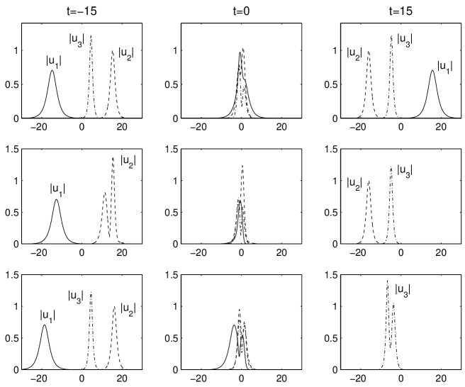
Figure 1: Soliton solutions in the three-wave system (14) corresponding to a single pair of zeros with rank sequence {1, 2} at time $t=-15,0$ and 15. Here, $k_{1}=1+i$, $|p_{02}^{(1)}\rangle=[-1,i,1-i]^{T}$, $|p_{01}^{(2)}\rangle=[1,0.5,-1]^{T}$. First row: $|p_{01}^{(1)}\rangle=[1,1+i,0.5]^{T}$; second row: $|p_{01}^{(1)}\rangle=[0,1+i,0.5]^{T}$; third row: $|p_{01}^{(1)}\rangle=[1,0,0.5]^{T}$.

To display these soliton solutions, we choose $k_{1}=1+i$, $|p_{02}^{(1)}\rangle=[-1,i,1-i]^{T}$, $|p_{01}^{(2)}\rangle=[1,0.5,-1]^{T}$. When $|p_{01}^{(1)}\rangle=[1,1+i,0.5]^{T}$ (the generic case), the solutions are plotted in the top row of Fig. 1. In two non-generic cases (where some elements of the $|p\rangle$ vectors vanish), $|p_{01}^{(1)}\rangle=[0,1+i,0.5]^{T}$ and $|p_{01}^{(1)}\rangle=[1,0,0.5]^{T}$, the solutions are plotted in the second and third rows of Fig. 1 respectively. We see that in the generic case, three sech waves in the three components interact and then separate into the same sech waves with their positions shifted. In other words, this is a $u_{1}(\mbox{sech})+u_{2}(\mbox{sech})+u_{3}(\mbox{sech})\rightarrow u_{1}(\mbox{sech})+u_{2}(\mbox{sech})+u_{3}(\mbox{sech})$ process. What happens is that the initial pumping ($u_{3}$) wave breaks up into two sech waves in the other two components ($u_{1}$ and $u_{2}$), while simultaneously the two initial $u_{1}$ and $u_{2}$ waves combine into a pumping sech wave. Thus this process is a combination of two sub-processes: $u_{3}\rightarrow u_{1}+u_{2}$ and $u_{1}+u_{2}\rightarrow u_{3}$. This phenomenon seems related to the rank sequence {1, 2} of the present solitons and the fact that, the rank sequence {1} itself describes the breakup of a pumping sech wave into two non-pumping sech waves, while the rank sequence {2} itself describes the reserve process. In the non-generic cases, these solutions can describe the $u_{1}(\mbox{sech})+u_{2}(\mbox{second-order})\rightarrow u_{2}(\mbox{sech})+u_{3}(\mbox{sech})$ process, the $u_{1}(\mbox{sech})+u_{2}(\mbox{sech})+u_{3}(\mbox{sech})\rightarrow u_{3}(\mbox{second-order})$ process (see Fig. 1, second and third rows), and many others. In the solutions of Fig. 1, the $a_{j}$ and $b_{j}$ parameters are such that $u_{2}<u_{3}<u_{1}$. If $u_{1}<u_{3}<u_{2}$, the processes will be exactly the opposite (see SIAM ). Thus our solutions can describe the opposite processes of Fig. 1 as well.

IV.2 Soliton solutions for two pairs of simple zeros

Here we derive soliton solutions corresponding to two pairs of simple zeros in the three-wave system (14). Some solutions belonging to this category have been presented in 3wavezakharov ; 3wave3 . But we will show that those solutions are only special (non-generic) solutions for two pairs of simple zeros. Below, the more general solutions for this case will be presented.

In this case, $r_{1}^{(1)}=r_{1}^{(2)}=1$. By using formula (81) for the case of involution (4) and with two pairs of zeros, we readily obtain that the number of free complex parameters in the solution is 6:

$${\cal N}_{\mathrm{free}}=2(3\times 1+1-1)=6.$$

Indeed, there are two $|p\rangle$ vectors in Eq. (114). Together with the two zeros $k_{1}$ and $k_{2}$, there are 8 complex parameters in the soliton solutions. However, the $2\times 2$ invariance matrix $B$ in this case is diagonal and has two free (diagonal) complex parameters.

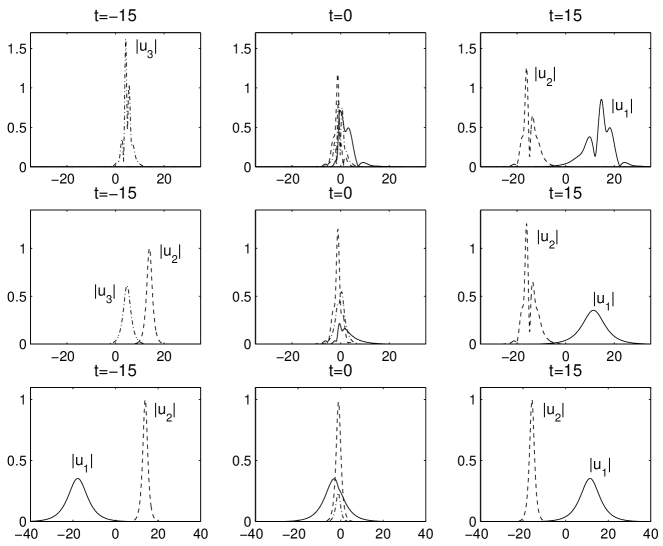
Figure 2: Soliton solutions in the three-wave system (14) corresponding to two pairs of simple zeros at time $t=-15,0$ and 15. Here, $k_{1}=1+i$, $k_{2}=-1+0.5i$. First row: $|p_{01}^{(1)}\rangle=[1,1+i,0.5]^{T}$, $|p_{01}^{(2)}\rangle=[1,0.5,-1]^{T}$; second row: $|p_{01}^{(1)}\rangle=[0,1+i,0.5]^{T}$, $|p_{01}^{(2)}\rangle=[1,0.5,-1]^{T}$; third row: $|p_{01}^{(1)}\rangle=[0,1+i,0.5]^{T}$, $|p_{01}^{(2)}\rangle=[1,0.5,0]^{T}$.

Three solutions, with $k_{1}=1+i,k_{2}=-1+0.5i$ and three different sets of $|p_{01}^{(1)}\rangle$ and $|p_{01}^{(2)}\rangle$ vectors, are displayed in Fig. 2. In the generic case where $|p_{01}^{(1)}\rangle=[1,1+i,0.5]^{T}$ and $|p_{01}^{(2)}\rangle=[1,0.5,-1]^{T}$ (see top row of Fig. 2), the solution describes the breakup of a higher-order pumping ($u_{3}$) wave into two higher-order $u_{1}$ and $u_{2}$ waves. This is analogous to solutions for a single pair of elementary zeros with algebraic multiplicity 2 (see SIAM ). In the non-generic case where $|p_{01}^{(1)}\rangle=[0,1+i,0.5]^{T}$ and $|p_{01}^{(2)}\rangle=[1,0.5,-1]^{T}$ (second row in Fig. 2), the present solutions can describe the $u_{2}(\mbox{sech})+u_{3}(\mbox{sech})\rightarrow u_{1}(\mbox{sech})+u_{2}(\mbox{second-order})$ process. This process has been seen in SIAM for elementary zeros as well. More interestingly, in the non-generic case when $p_{01}^{(1)}[1]=p_{01}^{(2)}[3]=0$, these solutions describe the elastic interaction of a sech $u_{1}$ wave with a sech $u_{2}$ wave (see bottom row of Fig. 2). These are precisely the soliton solutions presented in 3wavezakharov ; 3wave3 . We see that these solutions are simply non-generic solutions for two pairs of simple zeros.

IV.3 Soliton solutions for two pairs of higher-order zeros

Lastly, we consider two pairs of zeros, one simple and the other one elementary with the algebraic multiplicity 2. Let us say $k_{1}$ is the elementary zero, and $k_{2}\>(\neq k_{1})$ is the simple zero. Then the rank sequence for $k_{1}$ is {1, 1}, and the rank sequence for $k_{2}$ is $\{1\}$. Thus, $r_{1}^{(1)}=1$, $r_{2}^{(1)}=1$, and $r_{1}^{(2)}=1$. By formula (81) we have

$${\cal N}_{\mathrm{free}}=3(1+1)+1-(1+1)+3\times 1+1-1=8.$$

Indeed, in this case $s^{(1)}_{1}=2$ and $s^{(2)}_{1}=1$, hence there are 11 complex parameters in the soliton solutions (9 in the three $|p\rangle$ vectors, plus the two zeros $k_{1}$ and $k_{2}$). The invariance matrix $B$ can be found from the general formula (91) as

$$B=\left(\begin{array}[]{ccc}b_{11}&b_{12}&0\\ 0&b_{11}&0\\ 0&0&b_{33}\end{array}\right),$$

which has three free complex parameters. Thus ${\cal N}_{\mathrm{free}}=11-3=8$ as calculated above.

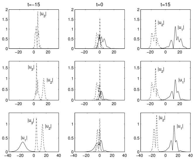
Figure 3: Soliton solutions in the three-wave system (14) corresponding to two pairs of zeros — one elementary with algebraic multiplicity 2, and the other one simple. Here, $k_{1}=1+i$ (elementary zero), $k_{2}=-1+0.5i$ (simple zero), and $|p_{02}^{(1)}\rangle=[-1,i,1-i]^{T}$. First row: $|p_{01}^{(1)}\rangle=[1,1+i,0.5]^{T}$, $|p_{01}^{(2)}\rangle=[1,0.5,-1]^{T}$; second row: $|p_{01}^{(1)}\rangle=[0,1+i,0.5]^{T}$, $|p_{01}^{(2)}\rangle=[1,0.5,-1]^{T}$; third row: $|p_{01}^{(1)}\rangle=[0,1+i,0.5]^{T}$, $|p_{01}^{(2)}\rangle=[1,0.5,0]^{T}$.

Three solutions, with $k_{1}=1+i,k_{2}=-1+0.5i$, $|p_{02}^{(1)}\rangle=[-1,i,1-i]^{T}$, and three different sets of $|p_{01}^{(1)}\rangle$ and $|p_{01}^{(2)}\rangle$ vectors, are displayed in Fig. 3. In the generic case (first row in Fig. 3), this solution describes the breakup of a higher-order pumping wave ($u_{3}$) into the other $u_{1}$ and $u_{2}$ components (both higher-order). In non-generic cases, it can describe processes such as $u_{2}(\mbox{sech})+u_{3}(\mbox{higher-order})\rightarrow u_{1}(\mbox{higher-order})+u_{2}(\mbox{higher-order})$ (second row of Fig. 3), $u_{1}(\mbox{sech})+u_{2}(\mbox{sech})+u_{3}(\mbox{sech})\rightarrow u_{1}(\mbox{higher-order})+u_{2}(\mbox{higher-order})$ (last row of Fig. 3), and many others. The inverse processes of Fig. 3 can also be described by choosing $a_{j}$ and $b_{j}$ values such that $u_{1}<u_{3}<u_{2}$ instead of $u_{2}<u_{3}<u_{1}$ in Fig. 3.

V Conclusion and Discussion

We have proposed a unified and systematic approach to study the higher-order soliton solutions of nonlinear PDEs integrable by the $N\times N$-dimensional Riemann-Hilbert problem. We have derived the complete solution to the Riemann-Hilbert problem with an arbitrary number of higher-order zeros, and characterized the discrete spectral data. As a result, the most general forms of higher-order multi-soliton solutions have been obtained in nonlinear PDEs integrable through the $N\times N$-dimensional Riemann-Hilbert problem. In other words, the most general reflection-less (soliton) potentials in the $N$-dimensional Zakharov-Shabat operators have been derived. The eigenfunctions associated with these reflection-less potentials are readily available from our soliton matrices. We have applied these general results to the three-wave interaction system, and new higher-order soliton and two-soliton solutions have been presented. These solutions reveal new processes such as $u_{1}+u_{2}+u_{3}\leftrightarrow u_{1}+u_{2}+u_{3}$. They also reproduce previous solitons in NMPZ84 ; 3wavezakharov ; 3wave3 ; SIAM as special cases. Our results can be applied to derive higher-order multi-solitons in the NLS equation and the Manakov equations as well, but this is not pursued in this article.

The results obtained in this paper are significant from both physical and mathematical points of view. Physically, our results completely characterized higher-order solitons and multi-solitons in important physical systems such as the three-wave interaction equation, the NLS equation and the Manakov equations. These higher-order solitons can describe new physical processes such as those displayed in Figs. 1 - 3. If these integrable equations are perturbed (which is inevitable in a real-world problem), our higher-order solitons then become the starting point for the development of a soliton-perturbation theory which could determine what happens to these higher-order solitons under external or internal perturbations hasegawa ; Yang00 . From the mathematical point of view, our results completely characterized the discrete spectral data of higher-order zeros in a general $N$-dimensional Riemann-Hilbert problem. These results will be useful for many purposes such as proving the completeness of eigenfunctions in a $N$-dimensional Zakharov-Shabat spectral problem with arbitrary localized potentials. The difficulty of such a proof is caused by higher-order zeros. With our results, this difficulty can be hopefully removed.

From a broader perspective, our results are closely related to many other physical and mathematical problems. For instance, the lump solutions in the Kadomtsev-Petviashvili I equation are given by the higher-order poles of the time-dependent Schrödinger equation. In ablowitz ; ablowitz2 , lump solutions corresponding to certain special higher-order poles were derived, but the most general lump solutions still remain an open question. Note that the time-dependent Schrödinger equation is an infinite-dimensional system compared to our present $N$-dimensional Riemann-Hilbert system. But the ideas used in this paper might be generalizable to the time-dependent Schrödinger equation as well. This remains to be seen.

VI Acknowledgments

This work was supported in part by NASA and AFOSR grants. J.Y. acknowledges helpful discussions with Jonathan Sands. V.S. would like to thank the University of Vermont for support of his visit during which this work was done.

Appendix A General Riemann-Hilbert problem with abnormal zeros

Here we show that our soliton matrices of section III can be generalized to the case of Riemann-Hilbert problem with abnormal zeros. However, due to the lack of important applications, we will show a simple example, which corresponds to a pair of zeros with different geometric multiplicities but the same algebraic multiplicity. Then we comment on the general case of several non-paired zeros.

Let us use the simplest example to show the idea behind generalization of our results to the general Riemann-Hilbert problem with abnormal zeros. Consider one pair of zeros $(k_{1},\overline{k}_{1})$ which have the same algebraic multiplicity 2 but different geometric multiplicities which are 1 and 2 respectively. The corresponding soliton matrices are as follows:

$$\Gamma(k)=I+\frac{(\overline{k}_{1}-k_{1})\left(|v_{1}\rangle\langle\overline{v}_{1}|+|v_{2}\rangle\langle\overline{v}_{2}|\right)}{k-\overline{k}_{1}},$$ (115)

$$\Gamma^{-1}(k)=\left(I+\frac{(k_{1}-\overline{k}_{1})|v_{1}\rangle\langle\overline{v}_{1}|}{k-k_{1}}\right)\left(I+\frac{(k_{1}-\overline{k}_{1})|v_{2}\rangle\langle\overline{v}_{2}|}{k-k_{1}}\right),$$ (116)

with the conditions that $\langle\overline{v}_{j}|v_{j}\rangle=1$, $\langle\overline{v}_{2}|v_{1}\rangle=0$ and $\langle\overline{v}_{1}|v_{2}\rangle\neq 0$. To verify that the above matrices are indeed inverse to each other it is enough to rewrite the matrix $\Gamma(k)$ in the form

$$\Gamma(k)=\left(I+\frac{(\overline{k}_{1}-k_{1})|v_{2}\rangle\langle\overline{v}_{2}|}{k-\overline{k}_{1}}\right)\left(I+\frac{(\overline{k}_{1}-k_{1})|v_{1}\rangle\langle\overline{v}_{1}|}{k-\overline{k}_{1}}\right)$$ (117)

and take into account that $P_{j}\equiv|v_{j}\rangle\langle\overline{v}_{j}|$ is a projector. Equations (116) and (117) are in fact the product representations of the form (27). Now let us show that there are exactly two solutions to $\langle\overline{p}|\Gamma^{-1}(\overline{k}_{1})=0$. Indeed, the corresponding null vectors are as follows

$$\langle\overline{p}_{1}|=\langle\overline{v}_{1}|,\quad\langle\overline{p}_{2}|=\langle\overline{v}_{2}|.$$ (118)

This is due to the fact that $\Gamma^{-1}(\overline{k}_{1})=(I-P_{1})(I-P_{2})$. But on the other hand there is just one solution to $\Gamma(k_{1})|p\rangle=0$: $|p_{1}\rangle=|v_{1}\rangle$. Suppose that there is another solution $|p_{2}\rangle$ to $\Gamma(k_{1})|p\rangle=0$ linearly independent from $|p_{1}\rangle$. We have then using formula (115) for $\Gamma(k_{1})$:

$$|p_{2}\rangle=|v_{1}\rangle\langle\overline{v}_{1}|p_{2}\rangle+|v_{2}\rangle\langle\overline{v}_{2}|p_{2}\rangle.$$ (119)

Thus $|p_{2}\rangle=a|v_{1}\rangle+b|v_{2}\rangle$. Using this in formula (119) we get, due to $\langle\overline{v}_{2}|v_{1}\rangle=0$ and $\langle\overline{v}_{1}|v_{2}\rangle\neq 0$,

$$a|v_{1}\rangle\langle\overline{v}_{1}|v_{2}\rangle=0,$$

which is a contradiction, since $a\neq 0$.

The soliton matrices given by formulae (115)-(116) have the following form in the standard notations of Lemma 1 of section III:

$$\Gamma(k)=I+\frac{|\overline{q}_{1}\rangle\langle\overline{p}_{2}|+|\overline{q}_{2}\rangle\langle\overline{p}_{1}|}{k-\overline{k}_{1}},$$ (120)

$$\Gamma^{-1}(k)=I+\frac{|p_{1}\rangle\langle q_{2}|+|{p}_{2}\rangle\langle q_{1}|}{k-k_{1}}+\frac{|p_{1}\rangle\langle q_{1}|}{(k-k_{1})^{2}},$$ (121)

where

$$|\overline{q}_{1}\rangle=(\overline{k}_{1}-k_{1})|v_{2}\rangle,\quad|\overline{q}_{2}\rangle=(\overline{k}_{1}-k_{1})|v_{1}\rangle,\quad\langle q_{1}|=(k_{1}-\overline{k}_{1})^{2}\langle\overline{v}_{1}|v_{2}\rangle\langle\overline{v}_{2}|,\quad\langle q_{2}|=(k_{1}-\overline{k}_{1})\langle\overline{v}_{1}|,$$

$$|{p}_{2}\rangle=\frac{|v_{2}\rangle}{(k_{1}-\overline{k}_{1})\langle\overline{v}_{1}|v_{2}\rangle}.$$

Notice that $\Gamma(k)$ has two blocks of size 1, while $\Gamma^{-1}(k)$ has one block of size 2. In general, for one pair of zeros with different geometric multiplicities, the soliton matrices have the structure of Lemma 1 but with different numbers of blocks in $\Gamma(k)$ and $\Gamma^{-1}(k)$, while the total number of the $|p\rangle$- and $\langle\overline{p}|$-vectors appearing in these matrices is the same and equals to the order of the pair of zeros. One can proceed to derive the representations similar to those in Lemma 4 for this case. Evidently, due to the way of the derivation, the formulae will be similar with the only difference in the number of blocks and block sizes in $\Gamma(k)$ and $\Gamma^{-1}(k)$.

In the more general case of the Riemann-Hilbert problem with abnormal zeros, the zeros can be non-paired (for instance, zero of order 2 in $C_{+}$ and two simple zeros in $C_{-}$). Formally, this case can be obtained by “splitting” some of the zeros inside pairs in several distinct zeros in the soliton matrices $\Gamma(k)$ and $\Gamma^{-1}(k)$ discussed above, since this limit is obviously regular (the geometric multiplicity of the zero to be split should be at least equal to the number of the generated in this way new zeros, thus providing for the needed number of blocks; formula (120), for instance, allows splitting of the zero $k=\overline{k}_{1}$ of $\Gamma^{-1}(k)$ into two simple zeros). Thus, the most general case can be handled starting from the case of just one pair of zeros, i.e., the case discussed above. The explicit expressions for the soliton matrices $\Gamma(k)$ and $\Gamma^{-1}(k)$ will involve similar relations between the numbers of zeros, their geometric multiplicities and the numbers and sizes of the $\nu$-blocks of vectors as those in lemma 1, though, obviously, with different particular numbers for each of the two matrices.

References

- (1) M. J. Ablowitz and H. Segur, Solitons and the Inverse Scattering Transform (SIAM, Philadelphia 1981).
- (2) S. P. Novikov, S. V. Manakov, L. P. Pitaevski, and V. E. Zakharov, Theory of Solitons: The Inverse Scattering Method (Consultants Bureau, New York, 1984).
- (3) L. D. Faddeev and L. A. Takhtajan, Hamiltonian Methods in the Theory of Solitons (Springer-Verlag, Berlin-Heidelberg-New York, 1987).
- (4) M. J. Ablowitz and P. A. Clarkson, Solitons, Nonlinear Evolution Equations and Inverse Scattering (Cambridge University Press, Cambridge, 1991).
- (5) V. E. Zakharov and A. B. Shabat, Funct. Anal. Appl. 8, 226 (1974).
- (6) V. E. Zakharov and A. B. Shabat, Funct. Anal. Appl. 13, 13 (1979).
- (7) R. Beals and R. R. Coifman, Commun. Pure Appl. Math. 37, 39 (1984).
- (8) R. Beals and R. R. Coifman, Commun. Pure Appl. Math. 38, 29 (1985).
- (9) R. Beals and R. R. Coifman, Inverse Problems 5 577 (1989).
- (10) R. Beals, P. Deift, and C. Tomei, Direct and Inverse Scattering on the Line, Math. Surv. Mono., 28, American Mathematical Society, Providence, R. I., 1988.
- (11) X. Zhou, SIAM J. Math. Anal. 20, 966 (1988).
- (12) X. Zhou, Commun. Pure Appl. Math. 42, 895 (1989).
- (13) T. Kawata, Riemann spectral method for the nonlinear evolution equations, p. 210, in Advances in Nonlinear Waves, ed. by L. Debnath, (Cambridge Univ. Press, Cambridge, 1984).
- (14) V. E. Zakharov and A. B. Shabat Sov. Phys. JETP 34, 62 (1972).
- (15) M. Wadati and K. Ohkuma, J. Phys. Soc. Jpn. 51, 2029 (1981).
- (16) H. Tsuru and M. Wadati, J. Phys. Soc. Jpn. 53 2908 (1984).
- (17) L. Gagnon, N. Stiévenart, Optics Lett. 19, 619 (1994).
- (18) N. Stiévenart, Solitons d’ordre supériore de l’équation de Schrödinger non-linéaire, MSc Thesis, Université Concordia, Montréal, Québec, Canada (1993).
- (19) D.E. Pelinovsky, J. Math. Phys. 39, 5377 (1998).
- (20) J. Villarroel and M.J. Ablowitz, Commun. Math. Phys. 207, 1-42 (1999).
- (21) M.J. Ablowitz, S. Charkravarty, A.D. Trubatch and J. Villarroel, Phys. Lett. A 267, 132-146 (2000).
- (22) V. S. Shchesnovich and J. Yang, Stud. Appl. Math. 110, 297 (2003).
- (23) V.E. Zakharov and A.B. Shabat, self-focusing and one-dimensional self-modulation of waves in nonlinear media.” Zh. Eksp. Teor. Fiz. 61, 118 (1971) [Sov. Phys. JETP 34, 62-69 (1972)].
- (24) V. E. Zakharov and S. V. Manakov, Sov. Phys. JETP Lett. 18, 243 (1973)
- (25) M. J. Ablowitz and R. Haberman, J. Math. Phys. 16, 2301 (1975).
- (26) V. E. Zakharov and S. V. Manakov, Zh. Eksp. Teor. Fiz. 69, 1654-1673 (1975) [Sov. Phys. JETP 42, 842 (1976)].
- (27) D. J. Kaup, Stud. Appl. Math. 55, 9 (1976).
- (28) S.V. Manakov, Zh. Eksp. Teor. Fiz. 65, 1392 (1973) [Sov. Phys. JETP 38, 248-253 (1974)].
- (29) A. S. Fokas, SIAM J. Math. Anal. 27, 738 (1996).
- (30) A. S. Fokas, Proc. R. Soc. Lond. A 453, 1411 (1997).
- (31) A. S. Fokas, J. Math. Phys. 41, 4188 (2000).
- (32) J. Leon, J. Math. Phys. 35, 3504 (1994).
- (33) A. Hasegawa and Y. Kodama, Solitons in optical communications. Clarendon, Oxford, 1995.
- (34) J. Yang, J. Math. Phys. 41, 6614 (2000).
- (35) V. S. Shchesnovich, J. Math. Phys. 43 (2002) 1460.