Irreversible quantum graphs

Abstract

Irreversibility is introduced to quantum graphs by coupling the graphs to a bath of harmonic oscillators. The interaction which is linear in the harmonic oscillator amplitudes is localized at the vertices. It is shown that for sufficiently strong coupling, the spectrum of the system admits a new continuum mode which exists even if the graph is compact, and a single harmonic oscillator is coupled to it. This mechanism is shown to imply that the quantum dynamics is irreversible. Moreover, it demonstrates the surprising result that irreversibility can be introduced by a “bath” which consists of a single harmonic oscillator.

1 Introduction

Quantum graphs emulate many properties of quantum chaotic systems, and their use is now widely spread in the physics and mathematics literature [1, 2, 3, 4, 5, 6, 7]. In many potential applications the physical systems are irreversible, and it is desirable to include this feature to quantum graphs, and thus enlarge their range of applicability.

The standard way to introduce irreversibility to a quantum system is by coupling it to a “bath” which consists of a set of “irrelevant” degrees of freedom. The bath dynamics is governed, however, by a well defined quantum hamiltonian [8, 9, 10, 11]. The enlarged system, composed of the original system and the bath, is a proper quantum system, with hamiltonian:

$$H=H^{system}+H^{bath}+W$$ (1)

$H^{system}$ and $H^{bath}$ are operators in the “system” and “bath” Hilbert spaces, respectively, and $W$ is the coupling. In the physics literature, irreversibility is generally associated with the bath having a continuous spectrum. The physical justification is based on the observation that the Poincaré recurrence time is infinite, or stated differently, the mean probability to return back to the initial state vanishes, which is a prerequisite for irreversibility. This argument can also be formulated mathematically. To simplify the presentation, assume that $H^{system}$ has a discrete spectrum, while the bath spectrum is continuous, with a spectral measure ${\rm d}\mu({\cal E})$ and $\delta$ normalized eigenfunctions $|\chi_{\cal E}\rangle$. Denoting by $\Psi_{\cal P}$ the projection of an eigenstate of $H$ on the system subspace, The Schrödinger equation can be reduced to

$$E\Psi_{\cal P}=H^{system}\Psi_{\cal P}+\lim_{\eta\searrow 0}\int{\rmd}\mu({\cal E})W_{\cal P}({\cal E})\frac{1}{E-{\cal E}+i\eta}W^{\dagger}_{\cal P}({\cal E})\Psi_{\cal P}\ ,$$ (2)

where $W_{\cal P}({\cal E})$ is the projection of $W|\chi_{\cal E}\rangle$ on the system subspace. Using the identity

$$\lim_{\eta\searrow 0}\frac{1}{x+i\eta}=-i\pi\delta(x)+{\cal P}\left(\frac{1}{x}\right),$$ (3)

one traditionally associates irreversibility with the operator

$$\Gamma(E)=-i\pi\int{\rmd}\mu({\cal E})\delta(E-{\cal E})W_{\cal P}({\cal E})W^{\dagger}_{\cal P}({\cal E})\ .$$ (4)

$\Gamma(E)$ is an anti hermitian operator, which introduces decay to the quantum time evolution. (This can be immediately shown when $\Gamma(E)$ can be approximated by an energy independent operator). Two important points must be emphasized. First, the discussion presented above is valid only when the bath spectrum is continuous. Second, $\Gamma(E)$ vanishes unless $E$ is in the support of the spectral measure. Similar expressions appear e.g., for the width of resonances in the Breit-Wigner theory [12].

Various approximations and models where used to extract the main features of quantum irreversibility as described by (4). Amongst the most popular is the harmonic-bath model where the bath consists of a continuous set of harmonic oscillators which are linearly coupled to the system degrees of freedom [10]. In this case, some of the integrations can be carried out, and using first order perturbation theory, the decay width introduced by the bath can be computed explicitly.

The purpose of the present work is to carry out the above program for a system which consists of a graph that is coupled linearly to a harmonic bath. The system will be described in section (2) and the corresponding Schrödinger operator will be discussed. Because of the form of the coupling, the question of finding a self-adjoint extension is not simple. In the present work, a physically motivated form of the Schrödinger operator is constructed, and the rigorous proof of its validity is given in an adjacent paper by Michael Solomyak [13].

Irreversibility is demonstrated by computing the vertex scattering matrices [1, 2], which are responsible for the transfer of current between the bonds of the graph (section (3)). For sufficiently strong coupling, the vertex scattering matrices are sub-unitary, which means that the total probability current is not conserved. Rather, it decreases upon scattering at the vertex. In other words, the quantum mechanical evolution is not unitary. The surprise is that this happens even when a single harmonic oscillator is coupled at the vertex! This mechanism should not be confused with what happens naturally when an additional lead to infinity is coupled to the vertex, and its effect on the original scattering is to draw current. This mechanism which induces an “escape width” to the graph dynamics is not what is considered here. Rather, non unitarity is due to the coupling to a harmonic oscillator.

The rest of the paper attempts to explain this result in physical terms. To this end, a simple graph is presented and solved approximately in section (4). Using this model, one can demonstrate and explain how the coupling of a single harmonic oscillator to a compact graph can modify the spectrum in a major way. If the coupling is week, the spectrum remains pure point. Beyond a critical strength, a continuous component appears in the spectrum. The appearance of the continuum occurs at the same value of the coupling constant at which the vertex scattering matrix becomes non unitary. A rigorous treatment of this spectral problem is also provided in Solomyak’s paper [13].

2 The Schrödinger operator on a graph and the coupling to a harmonic bath

A graph ${\cal G}$ consists of $V$ vertices connected by $B$ bonds according to the connectivity matrix $C_{i,j}$ which takes the value $1$ if the vertices $i,j$ are connected, and it vanishes otherwise. We assign the natural metric to the bonds, and associate a length $L_{b}$ to each. The position $x$ of a point on the graph is determined by specifying on which bond $b$ it is, and its distance $x_{b}$ from the vertex with the smaller index, $0\leq x_{b}\leq L_{b}$. Sometimes, it will be convenient to denote the bond connecting the vertices $i$ and $j$ by $(i,j)$.

In the absence of a harmonic bath, the Schrödinger operator can be defined in the following way: Let $x\in{\mathcal{G}}$ and $\Psi(x)$ a real valued and continuous function on ${\mathcal{G}}$, so that $\Psi(x)=\psi_{b}(x_{b})$ for $x\in b$, and $0\leq x_{b}\leq L_{b}$, where $\psi_{b}(x_{b})$ are twice differentiable in the interior of the bond. We restrict $\Psi(x)$ to be square integrable, and require that it is uniquely defined at the vertices. That is, all the functions $\psi_{b}$ which correspond to bonds connected at a vertex $i$ attain the same value $\phi_{i}$ at the common vertex. Given an arbitrary set of $V$ non-negative constants $\lambda_{i}$ one constructs the quadratic form:

$$L_{0}[\Psi]=\sum_{b=1}^{B}\int_{0}^{L_{b}}{\rm d}x_{b}\left|\frac{{\rm d}\psi_{b}(x_{b})}{{\rm d}x_{b}}\right|^{2}+\sum_{i=1}^{V}\lambda_{i}\phi_{i}^{2}\ .$$ (5)

The Euler-Lagrange variational principle selects the stationary solutions of the quadratic form, as the solution of the Schrödinger equation on the bonds:

$$\left(-\frac{{\rm d^{2}\ }}{{\rm d}x_{b}^{2}}-E\right)\psi_{b}(x_{b})=0\ ,$$ (6)

subject to the boundary conditions

$$\sum_{j=1}^{V}\left.C_{i,j}\frac{{\rm d\ \ \ \ }}{{\rm d}x_{(i,j)}}\ \psi_{(i,j)}(x_{(i,j)})\right|_{i}-\lambda_{i}\phi_{i}=0\ .$$ (7)

The summation is over all the bonds $(i,j)$ which emanate from the vertex $i$, and the derivatives are computed at the vertex. The quadratic form (5) is positive definite, and therefore, the boundary condition (7) provides a self adjoint extension of the Schrödinger operator for any choice of the (non-negative) constants $\lambda_{i}$. This operator determines the quantum dynamics of the “system”. One can extend this operator to non compact graphs, by adding bonds from the vertices to infinity. The corresponding scattering problem was amply discussed in the literature [2, 4, 5, 6, 7].

The bath degrees of freedom consist of $M$ harmonic oscillators with coordinates $q_{m}$, and frequencies $\omega_{m}$, subject to the hamiltonian

$$h_{m}=\frac{1}{2}\left(-\frac{{\rm d^{2}\ }}{{\rm d}q_{m}^{2}}+\omega_{m}q_{m}^{2}\right)\ ;\ q_{m}\in\mathbb{R}\ .$$ (8)

Denote ${\bf q}=(q_{1},\cdots,q_{M})$ and $H_{osc}=\sum_{m=1}^{M}h_{m}$. $H_{osc}$ is the “bath” hamiltonian. The coupling of the bath to the system is introduced by extending the quadratic form (5) to include the graph and harmonic bath coordinates. Consider $\Psi(x,{\bf q})=\psi_{b}(x_{b},{\bf q})\ {\rm for}\ x\in b$, where each of the $\psi_{b}(x_{b},{\bf q})$ is square integrable. For every value of ${\bf q}$, $\Psi(x,{\bf q})$ is uniquely defined at the vertices, where, at the vertex $i$ it assumes the value $\phi_{i}({\bf q})$. To each vertex, we assign a real valued function $\Lambda_{i}({\bf q})$, which is bounded at any finite domain of $\mathbb{R}^{M}$ and is allowed to diverge algebraically as $|{\bf q}|\rightarrow\infty$. (In the following, we shall refer to these functions as the “form-factors” ). We construct the quadratic form,

$$L_{osc}[\Psi] = \sum_{b=1}^{B}\int{\rm d}^{M}q\left\{\right.\int_{0}^{L_{b}}{\rm d}x_{b}(\ \left|\frac{{\rm d}\psi_{b}(x_{b},{\bf q})}{{\rm d}x_{b}}\right|^{2}+\psi^{*}_{b}(x_{b},{\bf q})H_{osc}\psi_{b}(x_{b},{\bf q}\ ))$$ (9)

$$+ \sum_{i=1}^{V}\Lambda_{i}({\bf q})\phi_{i}^{2}({\bf q})\left.\right\}\ .$$

Again, the Euler-Lagrange variational principle selects the stationary solutions of the quadratic form, as the solution of the Schrödinger equation on the bonds:

$$\left(-\frac{{\rm d^{2}\ }}{{\rm d}x_{b}^{2}}+H_{osc}-E\right)\psi_{b}(x_{b},{\bf q})=0\ ,$$ (10)

subject to the boundary conditions

$$\left.\sum_{j=1}^{V}C_{i,j}\frac{{\rm d\ \ \ }}{{\rm d}x_{(i,j)}}\ \psi_{(i,j)}(x_{(i,j)},{\bf q})\right|_{i}-\Lambda_{i}({\bf q})\phi_{i}({\bf q})=0\ .$$ (11)

The coupling between the “system” and the harmonic “bath” is thus mediated through the boundary conditions (11).

When the form-factors $\Lambda_{v}({\bf q})$ are non negative the quadratic form $L_{osc}[\Psi]$ is positive definite, and the Schrödinger operator (10), subject to the boundary conditions (11) is self adjoint. The standard linear coupling of harmonic baths is written as

$$\Lambda_{i}({\bf q})=\sum_{m=1}^{M}\Lambda_{im}\ q_{m}\ ,$$ (12)

with $\Lambda$ a $V\times M$ matrix with ${\bf q}$-independent real coefficients. Thus, $L_{osc}[\Psi]$ is not definite, and the proof that the system (10,11) is self-adjoint requires a special treatment, which is provided in [13]. The intuitive motivation behind this coupling scheme is that for a vertex with $v=2$, and a single harmonic oscillator, the boundary condition at the vertex is equivalent to an effective potential $\Lambda q\delta(x)$. This represents a well localized coupling of the particle on the graph to the harmonic oscillator.

3 The vertex scattering matrix

The boundary conditions at the vertices of graphs (without coupling to any harmonic oscillators) (7) impose the conservation of the probability current across the vertex. In other words, the boundary conditions at a vertex can be described by a unitary vertex scattering matrix which provides the linear relation between the amplitudes of the waves which imping upon the vertex and the waves scattered from it [1]. The vertex scattering matrix which corresponds to the boundary conditions (7) can be written explicitly as

$$\sigma^{(i)}_{b,b^{\prime}}(k)\ =\ -\delta_{b,b^{\prime}}+\frac{1+{\rm e}^{-2i\arctan\frac{\lambda_{i}}{v_{i}k}}}{v_{i}}$$ (13)

where $i$ denotes the vertex under consideration, $b$ and $b^{\prime}$ denote the bonds which emanate from the vertex, and $k={\sqrt{E}}$ is the wave number under consideration. Note that this $v_{i}\times v_{i}$ vertex matrix distinguishes only between reflection ($b=b^{\prime}$) and transmission between different bonds ($b\neq b^{\prime}$), which is independent of their specific identity. This is an expression of the fact that the boundary condition at the vertex is invariant under the interchange of the bonds. $\sigma^{(i)}_{b,b^{\prime}}(k)$ is symmetric, and its unitarity can be easily demonstrated. The single vertex, and the bonds emanating from it, is some times referred to as a “star-graph”.

Describing the quantum evolution and dynamics in terms of waves travelling freely along the bonds and scattered at the vertices, is a very useful concept in the theory of quantum graphs [1]. This is also true when harmonic oscillators are coupled, and we shall dedicate the rest of this section to the derivation of the the vertex scattering matrices which correspond to the boundary conditions (11). We shall show, that the coupling of the harmonic oscillators can have a profound effect - the vertex scattering matrix is not necessarily unitary for large values of the coupling $\Lambda$. Thus, the evolution on the graph is not conserving and hence irreversible!

To simplify the presentation, we consider the coupling to a single harmonic oscillator ($M=1$), and choose the units such that $\omega_{1}=1$. The spectrum of the combined system of a harmonic oscillator and the star graph without coupling, consists of overlapping continua with thresholds at $E_{n}=n+\frac{1}{2}$. Further simplification is achieved by considering energies in the interval $\frac{1}{2}<E<E_{1}$. In this energy range, and for $x$ values away from the vertex, only the ground state ($n=0$) of the harmonic oscillator is populated, which corresponds to purely elastic scattering. We shall compute the vertex scattering matrix by considering an incoming wave incident on the bond $b^{\prime}$ only.

Denoting

$$k^{2}=E-\frac{1}{2}\ \ ;\ \ k_{0}=k\ \ ;\ \ k_{n}=\sqrt{n-k^{2}}\ \ {\rm for}\ \ n\geq 1,$$ (14)

we expand the wave function in the complete orthonormal basis $\chi_{n}(q)$ of eigenfunctions of the harmonic oscillator hamiltonian $h_{1}(q)$. The bond wave functions are defined on the positive half line, with the common vertex at $x_{b}=0$. The expansion takes the form

$$\psi_{b}(q,x_{b})=\frac{1}{\sqrt{k_{0}}}\ \eta^{(b)}_{0}(x_{b})\ \chi_{0}(q)\ +\ \sum_{n=1}^{\infty}\frac{a^{(b)}_{n}}{\sqrt{k_{n}}}\ \eta^{(b)}_{n}(x_{b})\ \chi_{n}(q)\ .$$ (15)

The functions $\eta^{(b)}_{n}(x_{b})$ are given by

$$\eta^{(b)}_{0}(x_{b}) = \left\{\begin{array}[]{l}{\rm e}^{-ik_{0}x_{b}}+r\ {\rm e}^{ik_{0}x_{b}}\ \ \ \ \ b=b^{\prime}\\ \\ \ \ \ \ \ \ \ \ \ \ \ \ t\ {\rm e}^{\ ik_{0}x_{b}}\ \ \ \ \ b\neq b^{\prime}\end{array}\right.$$ (19)

$$\eta^{(b)}_{n}(x_{b}) = \ \ \ {\rm e}^{-k_{n}x_{b}}\ \ \ \ \ \ {\rm for}\ \ \ \ \ \ \ n\geq 1\ .$$

This way, $\Psi(x,q)$ corresponds asymptotically to an incoming wave together with scattered waves in the ground state channel. In all other (closed) channels, the wave functions are evanescent along the bonds. Note that in (19) we made use of the expected invariance of the scattering matrix under the interchange of bonds, so that $r$ stands for the reflection (diagonal) elements of the $\sigma$ matrix, and $t$ stands for the transmission (off-diagonal) elements of $\sigma$. Both parameters are independent of $b$.

The continuity at of $\Psi(x,q)$ at the vertex implies that the expansion coefficients ${a^{(b)}_{n}}$ are the same for all $b$, and therefore they will be denoted in what follows by $a_{n}$. Moreover,

$$1+r=t$$ (20)

Substituting in (11) and using (20), we get

$$t\ =\frac{2}{v}\ +\ \frac{\lambda}{2i}\frac{1}{\sqrt{k_{0}k_{1}}}\ a_{1},$$ (21)

and,

$$2a_{1}+\lambda\left(\ \ a_{2}\ \ \sqrt{\ \frac{2}{k_{1}\ k_{2}}}\ \right) = -\frac{\lambda}{\sqrt{k_{0}\ k_{1}}}\ t$$ (22)

$$2a_{n}+\lambda\left(a_{n+1}\sqrt{\frac{n+1}{k_{n}k_{n+1}}}+a_{n-1}\ \sqrt{\frac{n}{k_{n}k_{n-1}}}\ \right) = \ \ \ \ \ \ \ 0\ \ \ \ \ \ \ {\rm for}\ \ n\geq 2\ .$$

Where, $\lambda\equiv\frac{{\sqrt{2}}\Lambda}{v}$. (22) is an infinite set of linear, inhomogeneous equations, which are defined in terms of the infinite Jacobian matrix $J(k,\lambda)$ whose elements are explicitly given in (22). For large $n$

$$\sqrt{\frac{n}{k_{n}k_{n-1}}}=1+{\cal O}\left(\frac{1}{n}\right)\ .$$ (23)

We shall denote by $J_{0}(\lambda)$ the Jacobian matrix whose elements are defined by the equations with constant coefficients

$$2a_{n}+\lambda\left(a_{n+1}+a_{n-1}\right)=0\$$ (24)

which approximate (22).

Denoting by $G(z;k,\lambda)$ the resolvent

$$G(z;k,\lambda)=\frac{1}{J(k,\lambda)-z}$$ (25)

we get

$$a_{1}=-\lim_{\varepsilon\nearrow 0}G_{1,1}(i\varepsilon;k,\lambda)\frac{\lambda}{\sqrt{k_{0}\ k_{1}}}\ t.$$ (26)

Denote

$$\gamma(k,\lambda)=\frac{\lambda^{2}}{2\ k_{0}\ k_{1}}\lim_{\varepsilon\nearrow 0}G_{1,1}(i\varepsilon;k,\lambda)\ .$$ (27)

Substituting (26) in (21), we find

$$t\ =\ \frac{\frac{2}{v}}{1-i\gamma(k,\lambda)}\ \ \ \ ;\ \ \ \ \ r\ =\ t-1\ =\frac{(-1+\frac{2}{v})+i\gamma(k,\lambda)}{1-i\gamma(k,\lambda)}\ .$$ (28)

Note that when $\lambda=0$, the reflection and transmission coefficients reduce to (13) (with $\lambda_{i}=0$). The flux in the leads is conserved if $(v-1)|t|^{2}+|r|^{2}=1$, which is satisfied only if ${\cal I}m(\gamma(k,\lambda))=0.$ We shall now show that this happens if and only if $|\lambda|<1$. In other words, the dissipation of flux, or equivalently, quantum irreversibility occurs for $|\lambda|>1$.

Following [14], we associate to the Jacobi matrix $J$ the spectral measure $\mu(x;k,\lambda)$, defined by

$$G_{1,1}(z;k,\lambda)=\int\frac{{\rm d}\mu(x;k,\lambda)}{x-z}$$ (29)

Using the estimate (23), we find that the operator $(J-J_{0})$ is Hilbert-Schmidt. The main theorem in [14] guarantees that the absolutely continuous component of $\mu(x;k,\lambda)$ is supported in $\sigma(k,\lambda))=[2(1-|\lambda)|,2(1+|\lambda)|]$.

As long as $|\lambda|<1$, the support $\sigma(k,\lambda))$ is on the positive half-line. The limit $z=i\varepsilon\nearrow 0$ is straight forward, resulting in a real value for $\gamma(k,\lambda)$. Hence for $|\lambda|<1$ the flux in the $x$ channel is conserved.

When $|\lambda|>1$, the interval $\sigma(k,\lambda))$ includes the value $0$. To compute (27) we use (3), and get

$${\cal I}m\gamma(k,\lambda)=-\frac{\pi\lambda^{2}}{2k_{0}k_{1}}\varrho(0,\lambda)\neq 0$$ (30)

Where we write ${\rm d}\mu(x;k,\lambda)=\varrho(x,\lambda){\rm d}x$. Thus, conservation of flux is violated, which is equivalent to the onset of irreversibility. This is the main result of the present work. It proves the fact that ${\cal I}m\gamma(k,\lambda)\neq 0$, but it does not provide an explicit expression for $\gamma(k,\lambda)$. However, once it is computed numerically or approximately (see next paragraph) it can be used together with (28) to compute the vertex scattering matrix.

$$\sigma_{b,b^{\prime}}(k,\lambda)=-\delta_{b,b^{\prime}}+t(k,\lambda)$$ (31)

An approximate computation of the resolvent for energies in the vicinity of the elastic threshold ($E\gtrsim\frac{1}{2}$) can be obtained by replacing the Jacobi matrix $J(k,\lambda)$ by $J_{0}(\lambda)$. It is has constant values along its diagonals, and an exact solution of the inhomogeneous equations for $\lambda>1$ read

$$a_{n}={\rm e}^{in\alpha}\frac{t}{\sqrt{k_{0}k_{1}}}\ \ ;\ \ \cos\alpha=-\frac{1}{\lambda}$$ (32)

Thus,

$$\gamma(k,\lambda)\approxeq-\frac{\lambda}{k_{0}k_{1}}\ {\rm e}^{i\alpha}\ .$$ (33)

This is an explicit expression which can be directly used in(31).

Note that the valency $v$ of the vertex enters only though the scaled strength parameter $\lambda=\frac{\sqrt{2}\Lambda}{v}$.

When we relax the condition $E<E_{1}$ the same phenomenon will occur albeit it involves now the inelastic scattering channels, whose number is finite and determined by the total energy $E$. It gives no new insight, and therefore it will not be discussed further.

The fact that the spectrum of the Jacobi matrix is continuous played a crucial role in the previous arguments. It appears in a way which is reminiscent of the discussion of quantum irreversibility presented in the introduction.

Coming back to the observation that the ingoing current exceeds the total outgoing current, one naturally asks where can one find the rest of the probability density. This, and other relevant questions will be clarified in the next section.

4 A simple model

The star graph with $v=2$ is equivalent to the Schrödinger equation

$$\left[-\frac{\partial^{2}\ }{\partial x^{2}}+\frac{1}{2}\left(-\frac{\partial^{2}}{\partial q^{2}}+q^{2}\right)+\Lambda\ q\ \delta(x)\right]\Psi(x,q)=E\ \Psi(x,q)\ ,$$ (34)

with $(x,q)\in\mathbb{R}^{2}$. The boundary condition at the vertex is replaced by a term which can be interpreted as a potential, linear in $q$ and well localized in $x$. The Schrödinger equation describes a particle in the $(x,q)$ plane, moving under the action of the potential shown in figure (1), where the $\delta$ function is replaced by a narrow Gaussian.

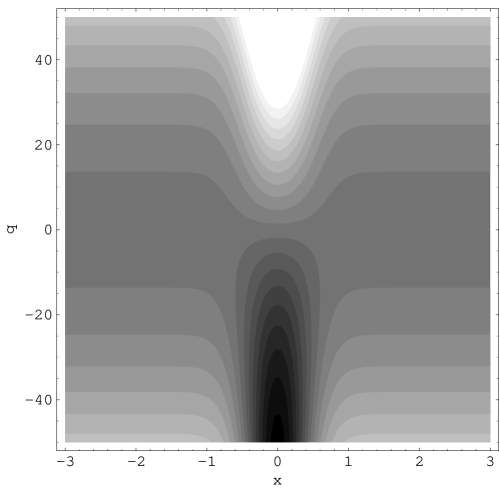
Figure 1: Grey level map of the potential in (34)

In this figure, the hight of the potential is indicated by the grey level, where black (white) marks the domains where the potential is most negative (positive). Consider now a particle moving in two dimensions and acted upon by this potential. Away from the domain of strong coupling, the potential is independent of $x$ and quadratic in $q$, thus forming a valley along the $x$ axis. Asymptotically, the particle moves with a constant speed in the $x$ direction, while oscillating in the $q$ direction. At the vicinity of $x=0$, the potential changes abruptly. Here a positive ridge (assuming $\lambda>0$) along the positive $q$ axis makes the $q>0$ domain inaccessible to the particle, while a down sloping valley pointing towards the negative $q$ axis, may attract the particle. As long as we use a finite Gaussian to simulate the $\delta$ potential, the quadratic potential in the $q$ direction will take over, and will form a barrier from which the particle will be reflected back and eventually the particle will find itself moving along the $x$ axis in either the positive or the negative directions. The limit where the Gaussian becomes a $\delta$ function, is delicate, and our computations show that it depends on the size of $\lambda$. Once $|\lambda|>1$, the effective potential valley extends to infinity, and it is sufficient to to draw flux in the $q$ direction without ever reflecting it back. Going back to the original way of looking at the problem, we can say that, with a finite probability, the “system” degree of freedom remains near the vertex at $x=0$ while the harmonic oscillator is excited in an outgoing stretching mode due to the strong interaction.

Another point of view can be obtained by studying the stationary wave function $\Psi(q,x)$ (15) at $x=0$. We consider its projection on the space of functions spanned by the oscillator states with $n\geq 1$, which correspond to evanescent modes in the $x$ direction,

$$\Psi(q,0)=\ \sum_{n=1}^{\infty}\frac{a_{n}}{\sqrt{k_{n}}}\ \chi_{n}(q)\ .$$ (35)

We use the approximate expression (32) for $a_{n}$, and replace the harmonic oscillator wave functions by their WKB approximation,

$$\chi_{n}(q) \approx \sqrt{\frac{2}{\pi}}\frac{\cos S(n)}{(2n+1-q^{2})^{1/4}}\ ,$$

$$S(n) = (n+\frac{1}{2})\left(\arcsin\frac{q}{\sqrt{2n+1}}+\frac{q}{\sqrt{2n+1}}(1-\frac{q^{2}}{2n+1})^{\frac{1}{2}}-\frac{\pi}{2}\right)\ .$$ (36)

Substituting in (35), and using the saddle point approximation to perform the sum, we obtain:

$$\Psi(x=0,q)\approx C\cdot\frac{{\rm e}^{-i\frac{q^{2}}{2}\tan\alpha}}{\sqrt{2\pi i\cos\alpha}}$$ (37)

Where $C$ is independent of $q$. This function is not square normalizable.

The simple computation above provides some heuristic evidence in support of the suggestion that the interacting system possesses a new continuum channel, where the particle can be trapped indefinitely. This issue is discussed in great detail and rigor in Solomyak’s paper [13]. In the sequel we shall present another variant of the simple model, where the onset of a continuum at $|\lambda|>1$ will be elucidated from yet another perspective.

Consider (34) subject to the boundary conditions

$$\Psi(x=-L_{1},q)=\Psi(x=L_{2},q)=0\ .$$ (38)

This Schrödinger operator describes a particle which is confined to the interval $[-L_{1},L_{2}]$ and a harmonic oscillator, which are coupled by an interaction which is very well localized at $x=0$, and is linear in the oscillator amplitude. The spectrum of the uncoupled ($\Lambda=0$) problem is pure point:

$$E_{n,m}=(n+\frac{1}{2})+\left(\frac{\pi}{L_{1}+L_{2}}\right)^{2}m^{2}\ \ ;\ \ n=0,1\cdots\ ;\ m=1,2,\cdots$$ (39)

We shall turn now to the case $\Lambda\neq 0$. We consider in particular the domain of energies $E<\frac{1}{2}$, just under the lowest energy of the unperturbed system. Again we expand $\Psi(x,q)$ in the complete orthonormal basis $\chi_{n}(q)$, and use the notation $k_{n}=+\sqrt{\frac{1}{2}+n-E}$ for $n=0,1,\cdots$.

$$\Psi(q,x)=\sum_{n=0}^{\infty}\frac{a_{n}}{\sqrt{k_{n}}}\ \eta_{n}(x)\ \chi_{n}(q)\ ,$$ (40)

where $\eta_{n}(x)$ satisfy the boundary conditions (38), are continuous at the origin, and normalized by $\eta_{n}(0)=1$. Explicitly,

$$\eta_{n}(x) = \left\{\begin{array}[]{l}\frac{\sinh k_{n}(L_{1}+x)}{\sinh k_{n}L_{1}}\ \ \ \ \ x\leq 0\\ \\ \frac{\sinh k_{n}(L_{2}-x)}{\sinh k_{n}L_{2}}\ \ \ \ \ x\geq 0\end{array}\right.\ \ \ \ \ \ \$$ (44)

These functions are evanescent away from the origin $x=0$. Substituting (40) in (34), we get a set of equations from which the coefficients $a_{n}$ are to be determined.

$$\gamma_{n}a_{n}+\lambda\left(a_{n+1}\sqrt{\frac{n+1}{k_{n}k_{n+1}}}+a_{n-1}\sqrt{\frac{n}{k_{n}k_{n-1}}}\right)=0\ ,$$ (45)

where, $\lambda=\frac{\Lambda}{\sqrt{2}}$ and

$$\gamma_{n}\ =\coth k_{n}L_{1}+\coth k_{n}L_{2}\ \ \ .$$ (46)

Equation (45) is a second order recursion relation with the boundary condition $a_{-1}=0$. The coefficients depend on the energy E, and the spectrum of the Schrödinger operator is determined as the values of $E$ for which the series $a_{n}(E)/\sqrt{k_{n}}$ is square summable. Before we proceed to analyze this further, we should point out that in the limit $n>>E$,

$$\sqrt{\frac{n}{k_{n}k_{n-1}}}=1+{\cal O}\left(\frac{1}{n}\right)\ \ \ ;\ \ \ \gamma_{n}=1+{\cal O}\left(\frac{1}{n}\right)\ .$$ (47)

Thus, (45) limits to the recursion relation with constant coefficients (24). This is of crucial importance to our discussion.

We shall now provide the heuristic arguments which show that for $|\lambda|<1$ the spectrum of the Schrödinger operator (34) retains its pure point character. However, for $|\lambda|>1$ it has a purely continuous component. Using the initial conditions $a_{-1}=0,\ a_{0}=1$, one can apply the exact recurrence relation (45) and obtain $a_{N}(E)$ for arbitrary large $N$. Chose $N$ such that for $n\geq N$ one introduces only a small error if one replaces (45) by (24). The solution of (24) can be written explicitly:

$$a^{approx}_{n}=A\ \xi^{n}+B\ \xi^{-n}\ \ \ ;\ \ \ \xi=\frac{1}{\lambda}\left(-1+\sqrt{1-\lambda^{2}}\right)\ ,$$ (48)

where $A,B$ are arbitrary constants, to be determined by the initial conditions.

For $|\lambda|<1$, $|\xi|<1$. Thus, to get a converging solution $B$ must vanish. The matching of the approximate series at $n=N$ requires

$$\xi=\frac{a_{N+1}(E)}{a_{N}(E)}\ ,$$ (49)

which is the spectral secular equation. Limiting our attention to the spectral interval $E<\frac{1}{2}$, and with $L_{1},L_{2}$ sufficiently large, we can chose $N=0$, and the secular equation reads,

$$\xi=\frac{a_{1}(E)}{a_{0}(E)}\ =-\frac{2}{\lambda}\left((\frac{1}{2}-E)(\frac{3}{2}-E))\right)^{\frac{1}{4}}.$$ (50)

Thus,

$$E=1-\frac{1}{2}\sqrt{1+\frac{1}{4}\left(1-\sqrt{1-\lambda^{2}}\right)^{4}}\ \ <\ \frac{1}{2}\ .$$ (51)

The approximate solution predicts the existence of a bound state of the system below the ground state of the unperturbed harmonic oscillator. This is rigorously proved in [13].

For $|\lambda|>1$,  $\xi=\exp(-i\arctan(\sqrt{\lambda^{2}-1})={\rm e}^{-i\zeta}$. Now, both terms in (48) contribute, and the secular equation reads,

$$\frac{a_{N+1}(E)}{a_{N}(E)}=\frac{A\ {\rm e}^{-i(N+1)\zeta}+B\ {\rm e}^{i(N+1)\zeta}}{A\ {\rm e}^{-iN\zeta}+B\ {\rm e}^{iN\zeta}}\ .$$ (52)

In contrast with the previous case, for every $E<\frac{1}{2}$, the matching condition are satisfied when

$$\frac{A}{B}=-{\rm e}^{2i(N+1)\zeta}\ \frac{1-\frac{a_{N+1}(E)}{a_{N}(E)}\ {\rm e}^{-i\zeta}}{1-\frac{a_{N+1}(E)}{a_{N}(E)}\ {\rm e}^{\ i\zeta}}\ .$$ (53)

Hence, the secular equation can be solved for every $E$, and the spectrum is continuous. Moreover, the $a_{n}(E)$ do not vanish in the limit of large $n$. Substituting the $a_{n}$ in (40), the resulting $\Psi(x,q)$ is bounded but not square integrable, which is typical for eigenfunctions in the continuous spectrum. We emphasize again the fact that the onset of irreversibility coincides with the appearance of a continuum. This result, which was illustrated above for the simple model, is general, and is entirely due to the typical form of the boundary conditions at the vertices.

A last comment is in order. Often, when facing an infinite set of equations of the type studied here, it is tempting to truncate them at a physically or computationally motivated point. In the present context, one would naturally attempt to truncate the space of closed channels, and perform the computations within the subspace of opened channel, exclusively. This would always result in a unitary description of the vertex scattering matrix, and the possibility of flux dissipation would be overlooked.

To summarize - the main lesson from this work is that genuine quantum flux dissipation and irreversibility can be induced by a single harmonic oscillator - the transmitted and the reflected fluxes do not add up to the incoming flux. This result is of general interest because it shows that in a strongly interacting system, continuum channels, which are absent in the uncoupled system and bath, can be opened by the interaction, and induce dissipation. At such instances, the perturbative approach to dissipation might not reflect the true nature of the problem.

5 Acknowledgements

First and foremost, the author wishes to thank Professor Michael Solomyak for the enjoyable discussions and exchanges which accompanied the work reported in the present paper. Professor Solomyak’s critical and pedagogical comments were most valuable. Part of this research was conducted when the author was a guest at the Mittag-Leffler Institute (MLI) and the Technical University (KTH) in Stockholm. Many thanks are due to Professor Ari Laptev and the MLI and KTH stuffs for their kind hospitality. Support from the Minerva Center for Nonlinear Physics, the Israel Science Foundation and the Minerva Foundation are acknowledged.

References

References

- [1] T. Kottos and U. Smilansky, Phys. Rev. Lett., 79: 4794, 1997.
- [2] T. Kottos and U. Smilansky. Ann. Phys. 274:76, 1999.
- [3] R. Carlson, Trans. Am. Math. Soc. 351:4069, 1999.
- [4] V. Kostrykin and R. Schrader J. Phys. A 32:595, 1999.
- [5] T. Kottos and U. Smilansky Phys. Rev. Lett. 85: 968, 2000.
- [6] P. Kuchment, Waves in Random Media 12 (2002), no. 4, R1-R24.
- [7] T. Kottos and U. Smilansky J. Phys. A 36 3501-3524 (2003).
- [8] W. Pauli Festschrift zum 60 Geburtstage A. Sommerfelds, Hirzel Verlag, Leipzig (1928), p. 30.
- [9] L. Van Hove Physica XXI:517,1955.
- [10] R.P. Feynman and A.R. Hibbs, Quantum mechanics and path integrals, McGraw-Hill, Inc. 1965.
- [11] H. Feshbach, Ann. Phys 5,357 (1958), and ibid 19, 287 (1962).
- [12] G. Breit and E. P. Wigner Phys. Rev. 49, 519 (1936).
- [13] M. Solomyak next paper in this issue.
- [14] R. Killip and B. Simon Sum rules for Jacobi matrices and their applications to spectral theory Annals of Mathematics, to appear (2003), arXiv math-ph/0112008.