Localization and Coherence in Nonintegrable Systems

Abstract

We study the irreversible dynamics of nonlinear, nonintegrable Hamiltonian oscillator chains approaching their statistical asymptotic states. In systems constrained by more than one conserved quantity, the partitioning of the conserved quantities leads naturally to localized and coherent structures. If the phase space is compact, the final equilibrium state is governed by entropy maximization and the coherent structures are stable lumps. In systems where the phase space is not compact, the coherent structures can be collapses represented in phase space by a heteroclinic connection of some unstable saddle to infinity.

keywords: Localized structures, statistical physics

1 Introduction

The formation of coherent structures by a continuing self focusing process is a widespread phenomenon in dispersive nonlinear wave systems. As a result of this process, high peaks of some physical field emerge from a low amplitude noisy background. For optical waves in Kerr-nonlinear media this results in a self-enhanced increase of light intensity in a small sector of a laser beam while the intensity in the neighborhood of this bright spot decreases [1]. Related phenomena occur in diverse systems from hydrodynamics to collapsing Langmuir waves in a plasma [2] and in numerical algorithms for partial differential equations [3], [4] .
A common feature of the wave dynamics of these systems is the comparable strength of the dispersion and the nonlinearity. But, self focusing phenomena are radically different in integrable and nonintegrable systems. In integrable systems [5], the peaks appear and disappear in a quasiperiodic manner reflecting the phase space structure of nested tori. This behavior is usually encountered on time scales that are short enough so that generic nonintegrable contributions to the dynamics may be neglected. Significant changes occur on time scales where the nonintegrability is relevant [6],[7]. The solution’s shape becomes more irregular [8],[9], [10],[11] and the periodic breathing of the peaks turns into a more persistent state. These peaks can merge into stronger ones while radiating low-amplitude waves. The irreversible character of the system becomes apparent and its behavior is driven by statistical mechanics [12],[13],[14] as the solution’s trajectory tries to explore more of the available phase space. As it does this, it must, at the same time, respect the preservation of conserved quantities. The phase space shell of constant conserved quantities determines the system’s most favorable macrostate and the resulting dynamics can lead to a local gathering of the amplitude while the system explores the phase space shell. We will see in situations with more than one conserved quantity that the spatial structure of the state which is statistically preferred now contains coherent peaks. If the phase space is compact, these peaks can be local , time independent and stable. If the phase space is not compact, the peaks can be collapsing filaments which produce singularities.
In this paper we study three systems which typify the focusing behavior observed in nonintegrable Hamiltonian systems with more than one conserved quantity, namely the Landau-Lifshitz equation for a classical Heisenberg spin chain, various versions of the discrete nonlinear Schrödinger equation, and a leapfrog discretization of the Korteweg-de Vries equation. Various modifications of these systems help to identify the role of the conserved quantities in the formation of coherent structures. The spatial discreteness of all these systems avoids fluctuations on infinitesimal scales.
The first case study investigates the Landau-Lifshitz equation for the classical spin chain in one spatial dimension. We study the long time behavior of those configurations in which most spins are close to the north pole. The two conserved quantities are the energy and the magnetic moment. Almost constant states undergo a series of modulational instabilities and the system begins to oscillate as if it were integrable. Nonintegrability, however, leads to non recurrence as localized peaks appear which merge from time to time leading to even larger peaks and radiating some energy. The phase space is compact, and one can compute to good accuracy the thermodynamic potentials of the system by separating the low-amplitude spin waves and the strongly nonlinear components. Depending on the initial value of the energy and the magnetization, entropy maximization leads to a state where some of the magnetization must be put into local structures bounded by domain walls for which the spin of each contained lattice point is close to the south pole. Numerical simulations very clearly support our simple analytical predictions which are based on thermodynamic considerations.
A close relative of the Heisenberg spin chain is found by taking the small amplitude limit where all spins are close to the north pole. Deviations are described by the focusing nonlinear Schrödinger equation. A similar dynamics is observed. In this study, we can also investigate the effects of exact integrability by using the Ablowitz-Ladik algorithm [15]. In these simulations, we find no irreversible behavior, no peak fusion, no relaxation, only quasi-periodic behavior. Likewise, we get qualitatively different results if we take a model which breaks the rotational symmetry and because of this the particle number is no longer conserved. As a consequence it is not necessary for the system to develop coherent structures in order to maximize its entropy as it no longer has to be concerned about the second constant of motion when its trajectory explores the accessible phase space.
The last case study concerns the leapfrog algorithm for the numerical integration of the Korteweg-deVries equation. It was observed in previous works [3],[4] that the leapfrog algorithm for the Korteweg-deVries equation always develops singularities. After (usually) a very long time, the amplitudes in some local neighborhood rapidly diverges. We demonstrate that this collapse again takes on an organized coherent form.
How and why does the system develop such local objects? The reason is again statistical. At an early stage, one can again observe the gathering of one of the conserved quantities in coherent structures. The system’s phase space is not compact, however, so that a strong nonequilibrium process prevails finally. We find a rapidly growing localized ’monster’-solution (so called because of its likeness in shape to the Loch Ness monster) that has a canonical structure. This solution can originate from coherent structures or, most frequently, from a long wave instability of the low-amplitude noisy background. We discuss the similarity of this process to the collapse behavior of the two dimensional focusing nonlinear Schrödinger equation, where the conservation laws necessitate a net inverse particle flux to small wavenumbers.
This paper is arranged as follows: In section 2, we present the Landau-Lifshitz equation, the discrete nonlinear Schrödinger equation and the leapfrog discretization of the Korteweg - de Vries equation and discuss some of their properties. In section 3 we present numerical studies of these equations. In particular, we study thermodynamic quantities during the focusing process. Their significance is also demonstrated by discussing modified equations with either more or with fewer conserved quantities as well as an equation of defocusing type. In section 4 we will give a statistical interpretation of the numerical findings. By computing the thermodynamic potentials of the spin-system, we find the connections between global features of the pattern and the conserved quantities. Macroscopic properties of the final state are computed. The discretized KdV equation has no such state of thermal equilibrium. We identify the rapid divergence of the amplitudes with the exploration of the non-compact phase space shell and we suggest that there is much similarity between this behavior and the condensation and collapse behavior seen in the focusing nonlinear Schrödinger equation.
Figures of similar contents are grouped together and their order sometimes deviates from the sequence of their references in the text.

2 Nonintegrable systems with constraints

2.1 Time-continuous systems

2.1.1 The Landau-Lifshitz equation

The anisotropic Heisenberg spin chain is particularly suitable for the study of self-focusing phenomena. This system contains the generic properties of equations of nonlinear Schrödinger type that lead to self-focusing and it is easy to investigate from the statistical point of view. The Landau-Lifshitz equation [16]

$$\dot{\bf S}_{n}={\bf S}_{n}\times(J({\bf S}_{n-1}+{\bf S}_{n+1})+S_{nz}{\bf e}_{z})$$ (1)

is a classical approximation of the dynamics of magnetic moments ${\bf S}_{n}=(S_{xn},S_{yn},S_{zn})$ at lattice sites $n$. $\dot{\bf S}_{n}$ is perpendicular to ${\bf S}_{n}$. Therefore the moduli of the spin vectors are conserved and one may set $|{\bf S}_{n}|=1$. The phase space of a chain of $N$ spins is a product of $N$ such spheres. $S_{z}$ the component of ${\bf S}$ along the rotational symmetry axis. The northern and southern hemispheres are equivalent since (1) is invariant under the transformation $(S_{xn},S_{yn},S_{zn})\rightarrow(-S_{xn},S_{yn},-S_{zn})$.
There are two trivial homogeneous equilibrium states where all the spins point either to the north pole $S_{z}=1$ or to the south pole $S_{z}=-1$. Throughout this paper we only consider solutions where most of the spins are close to the north pole.

2.1.2 The discrete nonlinear Schrödinger equation

The long-wavelength dynamics of spins which deviate slightly from the north pole $S_{z}=1$ is given by the focusing discrete nonlinear Schrödinger (DNLS) equation

$$i\dot{\phi}_{n}=J(\phi_{n+1}+\phi_{n-1}-2\phi_{n})+2|\phi_{n}|^{2}\phi_{n}$$ (2)

for small values of the complex amplitude $\phi=(S_{x}+iS_{y})/(1+S_{z})$. The spin chain may thus be regarded as a DNLS which is modified by higher order terms. The north pole is corresponds to $\phi=0$ while the south pole corresponds to an infinite amplitude.

2.1.3 Integrals of motion

The spin chain and the DNLS equation each have two conserved quantities:

1. The Hamiltonian of the DNLS equation ${\cal H}=\sum_{n}J(2\phi_{n}\phi_{n}^{*}-\phi_{n}\phi_{n+1}^{*}-\phi_{n}^{*}\phi_{n+1})-|\phi_{n}|^{4}$ is again obtained as the lowest order of the Hamiltonian of the spin chain ${\cal H}={\cal H}_{J}+{\cal H}_{a}=\sum_{n}J(1-{\bf S}_{n}{\bf S}_{n+1})+(1-S_{zn}^{2})/2$. The first contribution is a Heisenberg exchange coupling which is minimal for homogeneous solutions. The second part is an anisotropic energy that has minima at the poles $S_{z}=\pm 1$ and is maximal at the equator $S_{z}=0$. The stationary spin-up or spin-down solutions are the absolute energy minima. Fluctuations about these ground states give energy contributions per lattice site of the order of $|S_{x}+iS_{y}|^{2}$. Similarly, small fluctuations near by the equilibrium state $\phi=0$ of the DNLS contribute a coupling energy proportional to $|\phi|^{2}$. In contrast to the south pole state of the spin system, the energy of a solution $\phi\rightarrow\infty$ in the DNLS goes to minus infinity as $-|\phi|^{4}$.
   

2. The second conserved quantity of each system, the total magnetization ${\cal M}=\sum_{n}S_{zn}$ of the spin chain and the modulus-square norm (’particle number’) $\sum_{n}|\phi_{n}|^{2}$ of the DNLS, are related to the system’s rotational symmetry. The superposition of the Hamiltonian and this integral of motion yields a Hamiltonian in a rotating frame system. The negative magnetization $N-{\cal M}=\sum(1-S_{zn})\approx\sum|S_{xn}+iS_{yn}|^{2}/2$ corresponds to the particle number of the DNLS in the lowest order in amplitude. This ’particle number’ of the spin chain is zero for the north pole solution and it is two per lattice site for the south pole solution. In the DNLS, the particle number diverges for the state $|\phi|\rightarrow\infty$.

In order to contrast the generic behavior of such systems with those of (a) integrable systems and (b) systems not constrained by a second conservation law, we also consider two modified equations of motion. The first is the integrable Ablowitz-Ladik discretization of the one-dimensional nonlinear Schrödinger equation [15]). The second is an equation where the second integral is destroyed by a symmetry breaking field.
Low energetic solutions just above the ground states can be characterized by the ratio of the two integrals of motion, i.e. the energy per particle. This reveals a major difference between the spin chain and the DNLS. For fluctuations near the north pole or near $\phi=0$, the particle number is of the order of the energy so that this ratio is of order one for both systems. Spin-fluctuations near the south pole have the same energy but the second conserved quantity (’particle number’) is much higher so that the energy per particle is proportional to $|S_{x}+iS_{y}|^{2}$ and much less than $1$. Thus the spin chain has two states with low energies per lattice site, one ($S_{z}\approx 1$) with a higher energy per particle and one ($S_{z}\approx-1$) with a low positive energy per particle. This well-defined condensate state of low energy and high particle density is a mayor advantage of the spin chain.
In contrast, for infinitely high amplitude solutions of the DNLS that correspond to $S_{z}\approx-1$ solutions of the spin chain both the energy and the particle density go to infinity. The energy per particle diverges proportional to $-|\phi|^{2}$.

2.2 Time-discretized equation of motion

2.2.1 The leapfrog-discretization of the Korteweg-de Vries equation

The system of finite difference equations

$$\begin{array}[]{rcl}u_{m+1}(n)&=&v_{m}(n)\\ &&+\tau(u_{m}(n+2)-2u_{m}(n+1)+2u_{m}(n-1)-u_{m}(n-2)\\ &&-2(u_{m}(n+1)+u_{m}(n)+u_{m}(n-1))(u_{m}(n+1)-u_{m}(n-1)))\\ v_{m+1}(n)&=&u_{m}(n)\end{array}$$ (3)

is a leapfrog-type discretization in space and time of the completely integrable Korteweg-de Vries (KdV) equation $\dot{u}=u_{xxx}-6uu_{x}$ for the real amplitude $u(x,t)$. The leapfrog discretization is characterized by a central difference $\partial u/\partial t\rightarrow(u_{m+1}-u_{m-1})$. The factor $\tau$ of the spatial derivative is the time step size. The precursor $u_{m-1}$ is identified with the additional variable $v_{m}$ on the right side of the first equation. This scheme allows the simulation of the partial differential equation avoiding the amplitude dissipation that occurs in methods with numerical viscosity. The term $u_{m}(n+2)-2u_{m}(n+1)+2u_{m}(n-1)-u_{m}(n-2)$ is the standard discretization of $u_{xxx}$. The discretization of $uu_{x}$ was first suggested by Zabusky and Kruskal [17]. It involves a central difference in space $u_{m}(n+1)-u_{m}(n-1)$ and replaces $u$ by the average $(u_{m}(n+1)+u_{m}(n)+u_{m}(n-1))/3$.
This discretization suppresses fast-acting nonlinear instabilities. Discretizations that do not retain some of the original conservation laws lead to fast acting instabilities, since single modes diverge rapidly. For instance, the mode with the wavenumber $k=2\pi/3$ is driven by the nonlinear part of conventional discretizations of the KdV equation. In contrast, this mode is an exact solution of (3). Linear instabilities of the zero-solution can be avoided by a sufficiently small step-size $\tau<2/(3\sqrt{3})$.

2.2.2 Integrals of motion

The special feature of the spatial discretization (3) is that it preserves some of the original conserved quantities:

1. $<uv>=\sum_{n}u_{m}(n)v_{m}(n)=const.$ corresponds to the conserved quantity $\int u^{2}dx$ (’energy’ for shallow water waves) in the original KdV equation. The modulus-square norm $<u^{2}+v^{2}>=\sum_{n}u_{m}(n)^{2}+v_{m}(n)^{2}$ is not conserved.

2. $<u>=\sum_{n}u_{2m}(n)=\sum_{n}v_{2m+1}(n)$ and $<v>=\sum_{n}v_{2m}(n)=\sum_{n}u_{2m+1}(n)$ correspond to $\int udx$ (’mass’ for shallow water waves).

3 Numerical studies

We examine the formation of coherent structures numerically in various versions of the spin chain and the DNLS equation as well as the leapfrog integration scheme for the KdV equation. A typical scenario for the spin chain suggests that the final state mainly depends on the amount of the two conserved quantities provided by the initial conditions. Simulations of various modifications of the DNLS with either more of less integrals of motion clarify some more general conditions for this behavior. The simulations of the differential equations apply an Adams routine to a chain of 512 (and occasionally 4096) oscillators with periodic boundary conditions.

3.1 Dynamics of the spin chain

3.1.1 Benjamin-Feir instability and reversible dynamics

Plane wave solutions of the nonlinear Schrödinger equation are Benjamin-Feir unstable so that self-focusing is initiated by long wavelength modulations. Similarly, spin-wave solutions of the Heisenberg spin chain are unstable under long wavelength perturbations. For instance, the homogeneously magnetized solution ${\bf S}_{n}={\bf S}$ (Fig.1a)

Figure 1: Sketch of the spins for (a) the spatially homogeneous solution, (b) the spatially periodic solution resulting from a Benjamin-Feir instability, (c) the humps moving towards each other merging into compound peaks of spins pointing down (d).

that precesses about the symmetry axis ${\bf e}_{z}$ with the frequency $\omega=S_{z}$ is most unstable under perturbations with the wavenumber $k=\sqrt{1-S_{z}^{2}}/J$.
As a result of this instability, small perturbations lead to spatially periodic humps of spins approaching the equator while most of the spins come closer to the north pole (Fig.1b). The trajectory is close to a homoclinic orbit so that the solution returns to the almost homogeneous state after reaching the maximum amplitude.

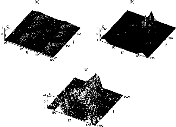
Figure 2: $S_{zn}$ as a function of the lattice site $n$ and time. (a) portrays the sector ($\alpha$) of Fig.3a, (b) is the sector ($\beta$); (c) is at ($\gamma$) of Fig.3b.

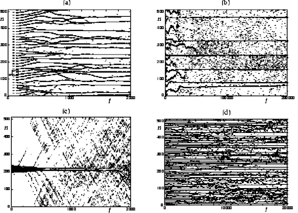
Figure 3: Integration of 512 spins $(J=0.4)$ with periodic boundary conditions; lattice sites where the spins deviate significantly from the north pole ($S_{z}<0.8$) are marked with dots. Integration over (a) 2000 and (b) 200,000 time steps with weakly perturbed homogeneous initial conditions $(S_{z}\approx\sqrt{0.84})$ (the profile of the z-magnetization at ($\alpha$, $\beta$, $\gamma$) are given in Fig.2); noisy short wave ($k=\pi$) inital conditions with a xenocryst of spins deviating strongly from the north pole over 2000 time steps (c); defocusing equation (negative sign of the potential), weak coupling ($J=0.1$) and noisy short wave ($k=\pi$) initial conditions over 20,000 time steps (d).

Fig.2a shows the profile of the z-magnetization in space and time for this solution which is almost periodic in space and time. Fig.3a shows the pattern of peaks (the sites of the spins that differ most from the north pole) as a function of time; Fig.2a is related to box ($\alpha$) of Fig.3a. Equidistant humps emerge and disappear periodically in time for $t<200$.

3.1.2 Merging of peaks and irreversible dynamics

The spatially periodic solution arising from the Benjamin-Feir instability is itself phase-unstable. As a result, the periodic pattern with the wavelength of the initial periodic mode becomes modulated on an even larger length scale so that the the gaps between the initially equidistant humps start to vary (Fig.1c). Fig.3a shows tiny variations of the distances between the humps as the humps start to move at $t\approx 60$ .
The most important phenomenon following the phase instabilities is the formation of coherent structures through mergings of peaks. Neighboring humps approaching each other finally merge into single peaks radiating small fluctuations. Fig.2b shows the profile of the magnetization during the fusion of humps of box ($\beta$) in Fig.3a. The original periodic solution is smooth, but the compound peak resulting from the merging has an irregular shape involving huge gradients both in space and in time. Its amplitude oscillates irregularly in time, but unlike the original periodic solution, it does not vanish any more completely. Even those humps that are situated remotely from the first merging processes become more persistent in time immediately so that they are traced by continuous lines in Fig.3a.
Subsequently, more humps fusing into compound peaks increase the average distance between neighboring peaks. The resulting compound peaks again merge with primary humps and with other compound peaks forming even stronger peaks (see point ($\gamma$) in Fig.3b with the magnetization profile of Fig.2c).

3.1.3 Final equilibrium state

The increasingly high amplitude of the compound-peaks enables some spins to overcome the energy barrier of the equator and to flip to the southern hemisphere (Fig.1d). (Fig.3b) shows that after $2\times 10^{5}$ time steps all peaks have merged into six down-magnetized domains that each consist of two or three lattice points. These peaks with $S_{z}\approx-1$ are embedded in a disordered state where the spins deviate only slightly from the north pole $S_{z}=1$. The final state is a two domain pattern where most of the spins are accumulated in huge up-magnetized domains while a few spins condense to small down-magnetized domains. The domain of the spin-wave fluctuations near to the north pole in the final state remains persistent even if the spin-down xenocrysts are removed artificially by flipping the down-spins up as $S_{z}\rightarrow|S_{z}|$.

3.1.4 Transfer of energy

The transition from the almost regular dynamics to the irreversible process during the merging of peaks is reflected in the share of the total energy of the two parts of the Hamiltonian. The coupling energy ${\cal H}_{J}=\sum(1-{\bf S}_{n}{\bf S}_{n+1})$ results from spatial inhomogeneities within each of the two domains and from the domain walls between them. The anisotropic energy ${\cal H}_{a}=\frac{1}{2}\sum(1-S_{nz}^{2})$ depends on the distance of the spins from the poles. Fig.4a shows the transfer of energy between the two parts of the Hamiltonian: The initial state contains no coupling energy and the anisotropic term is the only contribution. Some of this energy flows to the coupling part during the formation of the spatially periodic pattern.

Figure 4: (a): The evolution of the anisotropic energy $E_{a}$ and the coupling energy $E_{J}$ over 2000 time steps for 4096 spins with the initial conditions of Fig.3. (b): Numerical (points) and thermodynamic (line, see section 4.4) results of $E_{a}/E_{J}$ after long integration times.

This process is reversed while the system approaches the homogeneous state again so that energy is exchanged periodically between ${\cal H}_{a}$ and ${\cal H}_{J}$ (see the periodic behavior for short times in Fig.4a).
The transfer of energy from the anisotropy to the coupling becomes irreversible when the humps fuse into compound peaks. The share of coupling energy increases even more when compound peaks merge and an increasing number of spins overcomes the equator and settles down near to the south pole. In phase space, this process is related to Arnold diffusion. The trajectory disappears from the initial critical torus and explores more and more of the phase space. Finally, the system reaches an equilibrium state where the proportion of ${\cal H}_{a}$ and ${\cal H}_{J}$ saturates (Fig.4b). The bulk contribution to the coupling energy is due to the inhomogeneity within the north-pole domains and not the contribution from the domain walls.

3.2 Modified initial conditions

The systems energy and magnetization per spin given by the initial conditions determines the number of spins that point down after a long time. We study the final state for initial conditions with varying energies and with a modified magnetization profile. This gives strong numerical indications that the two integrals of motion (energy and the magnetization) are the key quantities that influence the final state.

3.2.1 Varying energies

Spin-wave like initial conditions $S_{xn}+iS_{yn}=\sqrt{1-S_{z}^{2}}\exp(ikn)$ with a given amplitude provide energies $E=N(1-S_{z}^{2})(\frac{1}{2}+J(1-cosk))$ depending on the wave number $k$ while the magnetization $M=NS_{z}$ is $k$-independent. The initial condition $k=0$ in the simulation described in Fig.2(a),(b) corresponds to the minimal energy $E=\frac{N}{2}(1-S_{z}^{2})/2$ that is possible for a given magnetization. The maximum energy $E=N(1-S_{z}^{2})(\frac{1}{2}+2J)$ corresponds to an excitation at the boundary of the Brillouin zone $k=\pi$ and any energy between these values can be obtained by a suitable spin wave.
We find that some of the spins condense near to the south pole eventually only if the energy is below a certain threshold $E_{eq}$ within this range. Fig.5 shows the magnetization of the south-pole

Figure 5: Numerical (dots) and analytical (line) results for the total magnetization $\sum_{n(S_{nz}<0)}|S_{nz}|$ of the spins in the southern hemisphere as a function of the total energy $E_{a}+E_{J}$ per spin for the system of Fig.1a. The initial conditions are $S_{z}=\sqrt{0.84}$, $S_{xn}+iS_{yn}=0.4\exp(ikn)$ with various wavenumbers $k$; waves with wavenumbers from $k=0$ to $k=\pi$ provide different amounts of coupling energy $E_{J}$ initially. The spin chain is integrated over 100000 time steps. For energies per spin below the threshold (equation (18)), some of the spins condense near to the south pole.

condensate as a function of the systems energy:

1. Oversaturated phase: Below the energy threshold $E_{eq}$, the number of down-spins is proportional to $E_{eq}-E$. The behavior in this is very similar to the scenario described before. The spatially homogeneous initial condition in the above simulations just leads to the highest possible proportion of the south-pole condensate.
   

2. Overheated phase: For high energies $E>E_{eq}$, no spins are flipped down so that this magnetization is zero. There is no south-pole condensate beyond this threshold; all spins end up in small fluctuations  near the north pole.

3.2.2 Modified magnetization profile

We have seen that only long-wavelength fluctuations create peaks. In contrast, high-energetic initial conditions with short wavelengths melt away such peaks of spins deviating significantly from the north pole. This occurs for an initial condition of a small-amplitude $k=\pi$ spin-wave (corresponding to the maximum energy in Fig.5) where the spins within a small domain are flipped to the southern hemisphere. Fig.3c shows the destruction of such a domain in a bath of $k=\pi$ waves. The system ends up in an irregular state where all spins are near to the north pole.

3.3 Modified equations of motion

The scenario we have described is widespread in dynamical systems and not a specific feature of the Landau-Lifshitz equation. A comparison of this scenario with self-focusing in related systems indicates that the main conditions for the emergence of coherent structures are

(i)

the low-amplitude dynamics is governed by an NLS-type of equation,

(ii)

the system is nonintegrable,

(iii)

there are two integrals of motion.

The first of these points basically characterizes the dynamics of nonlinear dispersive systems on long scales. The focusing DNLS is the system most closely related to the spin chain. Also the case of a defocusing nonlinearity will be considered. The importance of nonintegrability will be shown by the comparison to the integrable Ablowitz-Ladik discretization of the NLS equation. On the other side, we will study a system with broken rotational symmetry that only conserves the Hamiltonian.

3.3.1 Defocusing equation

The formation of coherent structures in discrete nonintegrable systems is not an exclusive property of ’focusing’ types of discrete NLS or Landau-Lifshitz equations. The Landau-Lifshitz equation $\dot{\bf S}_{n}={\bf S}_{n}\times((J({\bf S}_{n-1}+{\bf S}_{n+1})-{\bf S}_{nz}{\bf e}_{z})$ with a negative (’easy-plane’) anisotropy corresponds to the defocusing discrete NLS equation. For weak coupling constants ($J=0.1$), short wavelength ($k=\pi$) initial conditions produce coherent structures with spins condensing in the equator region where the anisotropic energy has now its minimum. Fig.3d shows this weak focusing process for the spin chain.

3.3.2 Discrete NLS equation

The focusing nonintegrable DNLS $i\dot{\phi}_{n}=J(\phi_{n+1}+\phi_{n-1}-2\phi_{n})+2|\phi_{n}|^{2}\phi_{n}$ has the properties (i)-(iii) just like the Heisenberg spin chain. Fig.6a shows the spatiotemporal pattern for the DNLS of lattice sites with high amplitudes that is very similar to the one described in section 3.1 (Fig.2a). Again, an unstable periodic pattern emerges from a phase-instability of the homogeneous state that is unstable itself.
The first and the second phase instability are well-known as direct consequences of (i) and (ii). The second phase instability has been studied in detail in the context of NLS equations. In phase space, it is related to degenerate tori with less than the maximum dimension. Such critical tori exist in integrable as well as in nonintegrable systems; they may be stable or unstable. The stability of these tori is related to double points in the spectral transform [10]. The spectrum of the Lax-operators has been analyzed both for an integrable and a nonintegrable version of the discrete NLS equation.
The fusions of humps lead to peaks with high amplitudes (Fig.6a) and finally high-amplitude xenocrysts emerge from a low-amplitude turbulent background. The whole process is very similar to the one of the Landau-Lifshitz equation (Fig.3a).

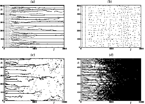
Figure 6: Integration of the various versions of the discrete nonlinear Schrödinger equation $(J=0.4)$ with 512 lattice sites and periodic boundary conditions. The inital conditions are $\phi_{n}=0.2$ plus noise, lattice sites with $|\phi|>0.25$ are marked with dots. (a): Integration of the DNLS over 2000 time steps; (b): Integration of the of the integrable version of the DNLS over 2000 time steps. (c): DNLS with a contribution $-2\phi_{n}$ and a symmetry breaking field $0.2\phi^{\prime}_{n}$ over 10,000 time steps; (d): DNLS with a symmetry breaking contribution $0.02\phi^{\prime}_{n}$ over 10,000 time steps.

The correspondence persists even in a domain where the additional nonlinear terms in the Landau-Lifshitz equation are not small. The DNLS-peaks may have different heights while the spin-peaks are always south-pole states.
The radiation of low-amplitude fluctuations during the merging of peaks is related to homoclinic chaos following the break up of Kolmogorov-Arnold-Moser tori. By discussing the Melnikov-function of the critical tori, [11] have detected homoclinic crossings in the nonintegrable NLS. The horseshoe of the homoclinic crossings creates the disorder following the fusion of two peaks.
A phenomenon similar to the merging of peaks was found in a continuous nonintegrable NLS equation [7]. Unlike solitons in integrable systems, collisions of solitary solutions of nonintegrable equations lead to a transfer of power from the weaker soliton to the stronger one while low amplitude waves are radiated. The resulting two-component solution contains a decreasing number of growing solitons immersed in a sea of weakly turbulent waves. In continuous systems, energy is drained by infinitesimal scales while the spatial discretization defines a minimal length scale.

3.3.3 Integrable discrete NLS equation

Homoclinic chaos as a source of radiation is absent in integrable systems. The comparison with the integrable discrete NLS $i\dot{\phi}_{n}=J(\phi_{n+1}+\phi_{n-1}-2\phi_{n})+|\phi_{n}|^{2}(\phi_{n-1}+\phi_{n+1})$ shows this implication of the nonintegrability (ii). The integrable NLS equation exhibits the primary phase instability, but not the fusing of neighboring peaks. While the dynamics is similar to the nonintegrable system initially, the peaks do not merge (Fig.6b). Consequently, no coherent structures evolve and the system does not settle down in a disordered equilibrium state. The quasiperiodic appearance of humps with relatively low amplitudes reflects the phase space structure of nested tori.

3.3.4 Particle nonconserving equation of motion

While the irreversible focusing process is a consequence of nonintegrability, it also depends on the existence of some remaining integrals of motion. The generation of coherent structures is very sensitive to perturbations that destroy one of the remaining integrals. The property (iii) may be changed by breaking the rotational symmetry with the contribution $\epsilon Re(\phi_{n})$ in the NLS equation. The equation is still of Hamiltonian type, but the modulus-square norm $\sum|\phi_{n}|^{2}$ is not conserved. Additional contributions $\sim\omega\sum|\phi_{n}|^{2}$ to the Hamiltonian and the corresponding term $\sim\omega\phi$ in the equation of motion $i\dot{\phi}_{n}=J(\phi_{n+1}+\phi_{n-1}-2\phi_{n})+\omega\phi_{n}+\epsilon Re(\phi_{n})+2|\phi_{n}|^{2}\phi_{n}$ are now relevant for the dynamics (in the symmetric case, this term just describes the same dynamics in different rotating frame systems; in the symmetry broken system, the external field $\epsilon$ is stationary in the system that rotates with the frequency $\omega$). Depending on the sign of $\omega$, two different scenarios are observed:

$\omega<0$:

The onset of self-focusing for small times is similar to the symmetric case. However, the peaks emerging from the fusing process disintegrate eventually into small amplitude fluctuations (Fig.6c).

$\omega\geq 0$:

The onset of the focusing process is again similar to the one with particle conservation, but after about 5000 time steps growing amplitude fluctuations lead to a disordered state. Unlike the rotationally symmetric system, high particle densities are not confined to small islands in a sea of low particle density fluctuations. The nonconservation of the particle number leads to high (but finite) particle density fluctuations everywhere (Fig.6d).

In the spin chain, similar effects can be reached with an external magnetic field that is perpendicular to the anisotropy axis ${\bf e}_{z}$ and an additional z-field. The Hamiltonian now contains the additional Zeeman terms $\epsilon S_{x}+\omega S_{z}$. Due to the broken rotational symmetry the total magnetization is no longer an integral of motion.

3.4 The leapfrog-discretization of the Korteweg-deVries equation

Iterations of the leapfrog-discretization of the Korteweg-deVries equation exhibit a scenario of merging peaks that is very similar to the one found in NLS or spin equations. However, the leapfrog system undergoes a rapid unbounded growth similar to the blow-up in twodimensional NLS systems. While the Heisenberg spin chain has a well-defined equilibrium, the leapfrog system allows us to study the conditions for blow-ups in constrained systems. We study this phenomenon for two initial conditions, the $k=2\pi/3$ mode with a strong correlation of $u$ and $v$, and for white noise with no correlation of $u$ and $v$. The system consists of 1020 lattice sites with periodic boundary conditions.

3.4.1 Correlated initial conditions

The monochromatic wave with the wavenumber $k=2\pi/3$ as initial condition yields an exact but phase-unstable [18] solution of the leapfrog-iteration (3a) for a sufficiently small step size.

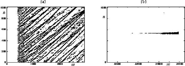
Figure 7: Iteration of the leapfrog-discretized KdV-equation (3) for a $k=2\pi/3$ wave (a) and for white noise initial conditions (b) with periodic boundary conditions. The amplitude of $u(n)=v(n)$ is $0.1$ initially in (a). Locations with high amplitudes (the sum of $u(n)^{2}$ over five subsequent steps is greater than 0.1) are marked with a dot. In (b), the threshold of $\sqrt{u^{2}+v^{2}}$ is is $0.045$ while the noise level $\sim 0.01$.

This mode is particularly relevant for a stability analysis since it is the fastest growing mode for a step size $\tau>2/(3\sqrt{3})$. Setting $u_{1}(n)=v_{1}(n)$ provides the maximum correlation of $u$ and $v$. The pattern of peaks Fig.7a (lattice sites with high $u(n)^{2}+v(n)^{2}$) emerges in a manner similar to the spin- and NLS-systems (Fig.3 and Fig.6):

1. Regular behavior: The initial low-amplitude wave is below the threshold to be traced in Fig.7 for $m<400$.

2. Merging humps: A phase instability of the initial $k=2\pi/3$ wave leads to a modulational pattern with a wavelength of about 20 lattice sites that reaches the threshold at $m\approx 400$ so that a spatially periodic pattern emerges for $400<m<600$. These periodic humps are wave packets of the initial short wave moving towards higher $n$. Similar to the spin- and NLS-systems, this pattern itself is slowly modulated. The humps approach each other and merge so that a decreasing number of peaks of increasing intensity survive. Solitary solutions that are high and fast sweep away slower ones. The peaks speed and amplitude increase while the width decreases during this process. They accumulate high amounts of the conserved quantity $<uv>$ just like the spin-down domains gather magnetization. Fig.8 shows the cumulated conserved

   

   Figure 8: Cumulated energy $\sum_{l=1}^{n}u_{m}(l)v_{m}(l)$ for the simulation of Fig.7 and Fig.9 as a function of the lattice site $n$ at the time steps $m=1$ and $m=2500$

   quantity $\sum_{l=1}^{n}u_{m}(l)v_{m}(l)$ as a function of $n$ (for $n=N$, it is conserved) at the beginning ($m=1$) and at $m=2500$ when the solitary waves have developed. While the conserved correlation $\sum u(n)v(n)$ is equally distributed in space initially, the formation of solitary wave packets gathers an increasing amount of the correlation in small xenochrysts immersed in uncorrelated low-amplitude fluctuations. Up to this point, the process is very similar to the self-focusing scenario presented in the spin- and NLS-systems.

3. Rapid divergence: However, despite the fact that for a long time the system appears to reach a statistically stationary state, in the end it is clear that no equilibrium is attained and the local amplitude rapidly diverges. At $m\approx 2960$, two peaks merge at $n\approx 420$ creating an all-time high of the amplitude that apparently exceeds a certain threshold locally. This highest peak now starts to grow rapidly so that the iteration is derailed within a few time steps. The features of this rapidly growing ’monster’-solution will be described in the next section.

Unlike the modulus square norm of the continuous KdV equation, $\sum u(n)^{2}$ is not conserved in the whole process. Fig.9a shows $\sum(u(n)+v(n))^{2}$ and $-\sum(u(n)-v(n))^{2}$

Figure 9: $\sum(u(n)+v(n))^{2}$ and $-\sum(u(n)-v(n))^{2}$ of the leapfrog-discretized KdV system as a function of time $m$ for the $k=2\pi/3$-wave (a) and for the white noise initial condition (b).

as a function of the time $m$. $\sum(u(n)+v(n))^{2}$ equals $4\sum u(n)v(n)$ initially while $-\sum(u(n)-v(n))^{2}$ starts at zero; the sum of both quantities $\sim<u(n)v(n)>$ is conserved. In the ’reversible’ range $m<400$ (i), both quantities increase and recur to their initial value periodically. As the merging of peaks starts (ii), they settle to almost constant values undergoing only a very slow increase. This behavior resembles Fig.4 up to the final blow-up (iii) where both quantities diverge rapidly.
Initial condition with a low amount of $<uv>$ lead to solitary solutions that do not reach the threshold for the blow up. Their growth ends when a few of them have absorbed this conserved quantity and move with the same speed. This state however is also unstable because of an instability to be described in the next section.

3.4.2 Uncorrelated white noise initial conditions

Uncorrelated low-amplitude white noise initial conditions $<uv>=0$ lead a creeping nonlinear process that suddenly ends up in the same sort of local rapid divergence of the amplitude. The time elapsing until the system blows up is inversely proportional to the square of the noise amplitude. For random white noise initial conditions with the same amplitude it is Poisson-distributed.
Fig.7b shows the spatiotemporal pattern of locations where the amplitude slightly exceeds the noise level. Unlike the correlated case, there is no spatiotemporal pattern of merging peaks. A change in the amplitude profile of the noise background is hardly detectable even shortly before the blow-up occurs. Again three phases of the dynamical behavior can be distinguished:

1. Regular behavior: For about 32000 time steps, the amplitudes are at the level of the noise imposed by the initial conditions. During this time, physical structures such as solitons can be simulated reliably when they are imposed by the initial conditions.

2. Creeping focusing process A weak non-moving maximum emerges at $m\approx 33500$, $n\approx 550$ and grows slowly. Fig.10 shows the low-pass filtered amplitudes of

   

   Figure 10: Profile of the peak evolving out of white noise (Fig.7b). Low-pass filtered amplitudes $u(n)$ (a) and $v(n)$ (b) at $m=33500$, $m=34000$, $m=34300$. (c): $u(n)$ at $m=34374$ two time steps before the iteration breaks down. The dotted line is the analytical solution. (d): $u(n)$ at $m=4100$, $m=4300$ and $m=4500$ for smooth initial conditions $v_{0}(n)=0$, $u_{0}(n)=0.01/\cosh^{2}(n-510)$ is very similar to the simulation (a).

   $u(n)$ (a) and $v(n)$ (b) of this structure at $m=33500$, $m=34000$, $m=34300$. The low pass filtered amplitude changes significantly with each time step, but very little with two subsequent time steps. Fig.11 shows the corresponding spectral density.

3. Rapid divergence After a slow growing process over about 1000 time steps this structure suddenly starts to grow rapidly and derails the iteration. Fig.10c shows $u(n)$ for this solution at $m=34374$. Fig.11 shows the spectral density of $<uv>$ at the time steps of Fig.10.

   

   Figure 11: Spectral density (defined as the Fourier-transform of the correlation $<u(n)(v(n+r)+v(n-r))+v(n)(u(n+r)+u(n-r))>$, $r\leq 100$ for the simulation of Fig.7b at the time steps of Fig.10. (a) shows the slowly growing solution that leads to the monster. (b): The correlation for the smooth initial conditions of the simulation 10d.

   This solution (which we call the ’monster’ solution because its spatial structure resembles the Loch Ness monster with several undulations of its tail sticking out of the water) appears to be the systems canonical trajectory towards infinite amplitudes.

Monsters are strongly localized: Left to the highest negative amplitude, the head of the monster, the amplitudes are close to zero. Right to the head, the amplitude of the zig-zag tail decreases rapidly. The monster moves to the left by one lattice site with each time step. There are also monsters that move to the right; their shape is related to left-moving monsters as $u(n)\rightarrow-u(-n)$. Most significantly, the amplitude of the monster is squared by every time step so that the monster grows as $exp(exp(m))$. Fig.7b shows a delta-shaped broadening zone of high amplitudes near the blow-up since the tail is growing while the head moves towards small $n$.
This solution can be calculated analytically. For a state $u_{m}(n)=Aa(n)$ with a high amplitude $A$, the linear terms of equation (3) may be neglected. We assume that the structure grows quadratically and moves to the right as $u_{m+1}(n)=2\tau A^{2}a(n-1)$. Setting $a(n)=0$ for $n>0$ and for negative odd $n$, we get the solutions $a(0)=1$, $a(-2)=(1-\sqrt{5})/2$, $a(-2n-2)=(1-\sqrt{1+4a(-2n)^{2}})/2$ as the solution of $a(n-1)=a(n-1)^{2}-a(n+1)^{2}$. The right moving solution is obtained by setting $a(n)\rightarrow-a(-n)$. The dotted line in Fig.10c shows this solution where the monster’s head is submerged.
Most significantly, the conserved quantities $<u>$, $<v>$ and $<uv>$ are zero for this solution; the monster needs no external food source for its growth. On the other side, it rapidly produces high amounts of $<u^{2}+v^{2}>$ (Fig.9b).
A blow-up with these characteristic features follows from various initial conditions. In the previous section we have described its evolution out of solitary solutions that emerge from a Benjamin-Feir type of instability and exceed a certain threshold after the merging process. It can also grow out of the noise between these solitary solutions or out of weak white noise through a much more dramatic type of instability.

4 Statistical analysis of the final state

In this section we will give a detailed interpretation of these results. The merging of peaks corresponds to an Arnold-diffusion process in phase space that transfers the trajectory from the initial critical torus to less distinctive parts of the shell of constant energy $<{\cal H}>=E$ and magnetization $<{\cal M}>=M$. The numerical findings indicate that the characteristics of the final solution are determined by the values of the integrals of motion; i.e. that the system reaches a thermodynamic equilibrium. One can therefore establish thermodynamic connections between macroscopic observables of the final solution and the integrals of motion. We will compute the equilibrium statistics of the system and compare the results to our numerical findings.

4.1 The partition function

4.1.1 Low-temperature approximation

The numerical findings suggest that for low energies the spins point to small regions near to the poles (Fig.1a) and avoid the region nearer to the equator. With $\sigma_{n}=\pm 1$ one may approximate spins near to the north- or south pole as

$$S_{nz}\approx\sigma_{n}(1-\frac{1}{2}(S_{nx}^{2}+S_{ny}^{2}))$$ (4)

Low amplitude fluctuations near the north pole are represented by $\sigma_{n}=1$ and small values of $S_{nx/y}$. The coherent structures with spins near to the south pole correspond to $\sigma_{n}=-1$. This matching height of all peaks is the main technical advantage of the spin chain. Assuming that $\sigma_{n}\sigma_{n+1}=1$ holds for almost all $n$ (i.e. the number of domain walls is small), one may approximate $\sum\sigma_{n}\sigma_{n+1}S_{nx/y}^{2}\approx\sum_{n}S_{nx/y}^{2}$. If all spins are close to the poles, the approximate Hamiltonian

$$\begin{array}[]{cccl}{\cal H}_{eff}&=&\sum_{n}&\frac{1}{2}(S_{nx}^{2}+S_{ny}^{2})+J(S_{nx}^{2}+S_{ny}^{2})\\ &&&-J(S_{nx}S_{n+1x}+S_{ny}S_{n+1y})\\ &&&-J\sigma_{n}\sigma_{n+1}\end{array}$$ (5)

represents a chain of coupled harmonic oscillators $(S_{nx},S_{ny})$ and a chain of Ising spins $\sigma_{n}$. The approximation holds if the energy is low and the magnetization is close to the maximum, i.e. $\sum(1-S_{nz})/N\ll 1$. It neglects the coupling between the oscillators $S_{nx/y}$ and the Ising spin $\sigma_{n}$ so that the Hamiltonian splits up into a spin-wave Hamiltonian ${\cal H}_{w}(S_{nx},S_{ny})$ and an Ising Hamiltonian ${\cal H}_{I}(\sigma_{n})$. ${\cal H}_{w}$ contains the lowest order terms of $S_{nx/y}$ and neglects anharmonic energy contributions of neighboring spins that point to the same hemisphere. ${\cal H}_{I}$ accounts for the coupling between up and down spins. In terms of the stereographic projection, ${\cal H}_{w}$ contains the terms that prevail for $|\phi|\ll 1$ while ${\cal H}_{I}$ allows for the contributions for $|\phi|\gg 1$. The nonlinearity is only reflected in the Ising magnet.
The magnetization as a second integral of motion may be approximated as

$${\cal M}_{eff}={\cal M}_{I}(\sigma)+{\cal M}_{w}(S_{x},S_{y})=\sum_{n}\sigma_{n}-\sum_{n}\frac{1}{2}(S_{nx}^{2}+S_{ny}^{2})$$ (6)

if most of the spins point to the north pole. Again this approximation neglects higher order terms in $S_{nx/y}$ and contributions $\sigma_{n}S_{nx/y}^{2}$ with $\sigma_{n}=-1$.

4.1.2 Grandcanonical partition function

The phase space surface on which ${\cal M}$ and ${\cal H}$ are constant can be computed most easily using the grand partition function

$$y(\beta,\gamma)=\int e^{-\beta({\cal H}_{eff}-\gamma{\cal M}_{eff})}d\Gamma$$ (7)

with two parameters $\beta$ and $\gamma$. Unlike the canonical ensemble [19], the grand canonical ensemble reflects the second integral of motion by the parameter $\gamma$ that controlls the system’s magnetization. $\beta$ is the inverse temperature while $\gamma$ is an equivalent of a magnetic field or chemical potential. The exponent in (7) is a sum ${\cal H}_{eff}-\gamma{\cal M}_{eff}=({\cal H}_{w}-\gamma{\cal M}_{w})+({\cal H}_{I}-\gamma{\cal M}_{I})$ of a spin-wave contribution

$${\cal H}_{w}-\gamma{\cal M}_{w}=\sum_{n}\frac{J}{2}((S_{nx}-S_{n+1x})^{2}+(S_{n+1y}-S_{n+1y})^{2})+\frac{1+\gamma}{2}(S_{nx}^{2}+S_{ny}^{2})$$ (8)

that depends only on $S_{nx},S_{ny}$ and an Ising contribution

$${\cal H}_{I}-\gamma{\cal M}_{I}=J\sum_{n}(1-\sigma_{n}\sigma_{n+1})-\gamma\sum\sigma_{n}$$ (9)

that depends only on $\sigma_{n}$. The partition function (7) of the whole system is the product $y=y_{w}y_{I}$ where $y_{w}$ is obtained by an integration over the variables $S_{nx},S_{ny}$ while $y_{I}$ is a sum of the configurations of the Ising spins $\sigma_{n}$. The grand partition function of the $N$ Ising spins

$$y_{I}=(cosh(\gamma\beta)+\mu)^{N}$$ (10)

with the abbreviation $\mu=\sqrt{sinh^{2}(\gamma\beta)+e^{-4J\beta}}$ is just the canonical partition function of an Ising magnet in an external field $\gamma$. The linear dynamics of $S_{nx}$ and $S_{ny}$ has the symplectic structure $\dot{S}_{nx/y}=\pm\partial{\cal H}_{w}/\partial S_{ny/x}$ so that a phase space volume element may be approximated as $d\Gamma=\prod dS_{xn}dS_{yn}$. For $\beta\gg 1$, the grand partition function of the spin waves can be obtained by integrating of $d\Gamma=\prod dS_{xn}dS_{yn}$ from minus to plus infinity. Using the abbreviation $A=\sqrt{\frac{J}{2}+\frac{1+\gamma}{8}}+\sqrt{\frac{1+\gamma}{8}}$ the Gaussian integrals yield

$$y_{w}(\beta,\gamma)=(\frac{\pi}{A^{2}\beta})^{N}$$ (11)

4.2 Thermodynamic relations

4.2.1 Energy and magnetization

The thermodynamic properties of the equilibrium state may be derived from the grand partition function $lny(\beta,\gamma)=lny_{w}+lny_{I}$. The parameters $\beta,\gamma$ and the conserved quantities $<{\cal H}>=E$, $<{\cal M}>=M$ are connected by

$$\begin{array}[]{ccl}M&=&M_{w}+M_{I}\\ &=&\frac{1}{\beta}\frac{\partial}{\partial\gamma}(ln(y_{w})+ln(y_{I}))\\ &=&N(-\frac{1}{\beta\lambda}+\frac{sinh(\gamma\beta)}{\mu})\end{array}$$ (12)

$$\begin{array}[]{ccl}E&=&E_{w}+E_{I}\\ &=&(\frac{\gamma}{\beta}\frac{\partial}{\partial\gamma}-\frac{\partial}{\partial\beta})(ln(y_{w})+ln(y_{I}))\\ &=&\frac{N}{\beta}(1-\frac{\gamma}{\lambda})+\frac{2NJe^{-4J\beta}}{cosh(\gamma\beta)\mu+\mu^{2}}\end{array}$$ (13)

with $\lambda=\sqrt{4J(1+\gamma)+(1+\gamma)^{2}}$. The partition function is valid for small energies per lattice site $E/N\ll 1$ and for small mean deviations $1-M/N\ll 1$ of the spins from the north pole. Low amplitude initial conditions without huge deviations from the north pole correspond to magnetizations in the interval $1-E/N\leq M/N\leq 1-E/(N(1+4J))$. The lower bound corresponds to a spatially homogeneous initial condition while a wave with $k=\pi$ defines the upper bound.
$M_{I}$, $E_{I}$, $M_{w}$, $E_{w}$ are the physically most interesting quantities:

1. is the magnetization of the Ising system and measures the total extent of the coherent structures. At its maximum $M_{I}=N$, all spins point up while smaller values $N>M_{I}>M$ indicate the existence of coherent structures where the spins point down

2. is the positive coupling energy of the domain boundaries and determines the number of coherent structures

3. is the negative magnetization of small fluctuations

4. is the positive energy of small fluctuations and comprises a coupling term and an anisotropic term

These quantities can be found by computing $\beta$ and $\gamma$ as functions of $E$ and $M$ and then plugging $\beta$ and $\gamma$ in the expressions for $E_{I}$, $M_{I}$, $E_{w}$, $M_{w}$. (12), (13) can be solved analytically for the low energy case $E/N\ll 1$. The solution (Fig.12) is qualitatively different in the ’oversaturated phase’ with $M<M_{eq}$ and in the ’overheated phase’ $M_{eq}<M<M_{\pi}$ with $M_{eq}=N-E/\sqrt{1+4J}$:

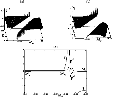
Figure 12: The temperature $\beta^{-1}(M_{w},E_{w})$ (a) and the chemical potential $\gamma(M_{w},E_{w})$ (b) as obtained from the equations (12) and (13). The energy is fixed as $E_{w}=0.1$ in (c).

4.2.2 Oversaturated phase $M<M_{eq}$:

1. The temperature $\beta^{-1}\approx E/N\ll 1$ is almost independent of $M$
   

2. The chemical potential $\gamma\approx Ee^{-2JN/E}/\sqrt{2N(M_{eq}-M)}\approx 0$ is exponentially small unless the magnetization comes very close to the transition point where this approximation breaks down.
   

3. Almost the total energy $E_{w}\approx E$ is absorbed by the fluctuations while the surface energy $E_{I}\sim e^{-2JN/E}\approx 0$ is exponentially small.
   

4. The fluctuations share $M_{w}\approx-E/(\sqrt{1+4J}N)$ of the magnetization is independent of the total magnetization. The remainder of $M-N$ is absorbed by the spins that are flipped down. The share of spins that is flipped down is at most of the order of the energy.

4.2.3 Overheated phase $M_{eq}<M<M_{\pi}$:

1. The temperature

   $$\beta^{-1}=\frac{(E+M-N)(4J(M-N)+E+(M-N))}{(4J(M-N)+2(E+(M-N)))N}$$ (14)

2. and the chemical potential

   $$\gamma=\frac{(E+M-N)^{2}}{4J(M-N)^{2}+2(E+M-N)(M-N)}-1$$ (15)

   both have a singularity at $M_{s}=N-E/(2J+1)$. The temperature is positive between $M_{w}=M_{0}$ and the singularity because the number of accessible states grows with the energy in this range. Beyond the singularity, more energy leads to a decreasing number of states so that the temperature is negative.
   

3. The spin waves $E_{w}\approx E$ again absorb the bulk of the energy while $E_{I}\sim e^{-2JN/E}\approx 0$.
   

4. The Ising-magnetization is near to its maximum $M_{I}\approx N$ independently of $M$. Fluctuations contribute the magnetization $M_{w}\approx-E/\lambda$

4.2.4 Transition at $M_{eq}$

The solution for $M_{I}$ explains the transition behavior of Fig.5 (section 3.2.1) and the emergence of coherent structures quantitatively. While the oversaturated phase corresponds to long spin-wave initial conditions, the thermodynamic equilibrium state is characterized by coherent structures, i.e. spins pointing to the south pole: Below the threshold $M_{eq}$, the Ising-magnetization $M_{I}$ deviates significantly from its maximum $M_{I}=N$ and the number of spins that point down increases linearly with $M_{eq}-M$. Above the transition the Ising magnetization deviates very little from its maximum $M_{I}=N$, so there are no coherent structures.
In both phases almost all energy is absorbed by low amplitude fluctuations. The surface energy $E_{I}$ is exponentially small, so that the spins form a very small number of domains. The higher number of domains obtained numerically indicates that the system does not thermalize completely on reasonable time scales.
As the spins interact only pairwise with a short range in one dimension, the transition between the two phases is of diffuse type and not a genuine phase transition. $\gamma$ and $M_{I}$ are analytic functions. The slope of $\gamma$ increases rapidly within a small interval $\sim e^{-4JN/E}$ at $M_{eq}$ so that the transition approaches a phase transition as the energy goes to zero.

4.3 The entropy

4.3.1 The shape of the entropy function

The thermodynamic reasons for coherent structures are best described in terms of the systems entropy. The conserved quantities $M$ and $E$ are known from the initial conditions rather than the arguments $\beta,\gamma$ of the grand partition function. Consequently, the entropy as a function of $M$ and $E$ is the appropriate thermodynamic potential. The entropy follows from the grand partition function by two Legendre transformations

$$\begin{array}[]{ccl}S&=&ln(y)+\beta(E-\gamma M)\\ &=&(1-\beta\frac{\partial}{\partial\beta})ln(y)\end{array}$$ (16)

Both the spin-waves and the Ising system contribute to the entropy. The two systems can get different shares $E_{I}$, $M_{I}$ and $E_{w}$, $M_{w}$ of the two conserved quantities $E$ and $M$. The entropy of the Ising has the form $\sim-E_{I}ln(E_{I}/N)$. The spin-wave entropy per lattice site is given by $S_{w}/N=ln\Omega$ where the total number of accessible microstates is $\Omega^{N}$ with

$$\Omega=\frac{(E_{w}+(1+4J)M_{w})(E_{w}+M_{w})}{NM_{w}}$$ (17)

So the entropy of small fluctuations depends on the energy as $\sim Nln(E_{w}/N)$. Both systems are coupled thermally, so they have matching temperatures $\beta^{-1}$. Using $\beta=\frac{\partial S}{\partial E}$ we reestablish the fact that the Ising energy $E_{I}/N\sim e^{-2J\beta}$ is exponentially small compared to the energy of the fluctuations $E_{w}/N\sim\beta^{-1}$ for low energies. The resulting Ising entropy is again exponentially small $S_{I}\sim e^{-2J\beta}$ compared to the spin-waves contribution $S_{w}\sim-ln\beta+const$.
Consequently, the main part of the entropy arises from the degrees of freedom of waves with small amplitudes while the Ising system only provides an almost constant contribution. The Ising system can absorb some of the systems magnetization without changing its energy and entropy significantly. By doing that, the fluctuations share of magnetization can also change allowing the fluctuations to maximize their entropy. The maximum of $S_{w}=Nln\Omega$ as a function of $E_{w}$ and $M_{w}$ is approximately the total entropy maximum.
Fig.13a shows the number of states per lattice site $\Omega$

Figure 13: $\Omega$ for the spin chain as a function of $E_{w}$ and $M_{w}$: (a) focusing equation with $J=0.4$. The focussing process corresponds to the arrow on the left slope, the arrow on the crest sketches the merging of peaks. The arrow on the right slope represents the destruction of coherent structures by short-wavelength fluctuations. (b) defocusing case for $J=0.1$ and $J=0.4$. The line $M_{\pi}$ crosses $E_{w}=0$ for $4J-1=0$.

of the fluctuations as a function of $M_{w}$ and $E_{w}$. It has the shape of a crest ascending towards higher energies. All possible small-amplitude states corresponding to positive $\Omega$ are in a triangular region limited by two highly ordered solutions ($M_{0}=-E_{w}$ and $M_{\pi}=-E_{w}/(4J+1)$) and by the systems total energy $E_{w}=E$.
The area between the lines $M_{0}$ and $M_{eq}$ again represents the oversaturated phase. The rim $M_{0}=-E_{w}$ with $\Omega=0$ corresponds to a monochromatic wave with $k=0$. Long wavelength solutions (which are also representative for continuous systems) are located at the slope near to this line. Such fluctuations have a low ratio $E/(N-M)$. Solutions that include high peaks may have even smaller values $M<N+M_{0}$. However, their inert down-magnetized domains have little influence on the thermodynamics and these states are similar to the ones at $M_{0}$.
The overheated phase is located between the lines $M_{eq}$ and $M_{\pi}$. The rim $M_{\pi}=-E_{w}/(4J+1)$ with $\Omega=0$ represents a wave $k=\pi$ at the boundary of the Brillouin zone. This wave has the highest ratio $E/(N-M)$ of all solutions.
The systems total energy $E_{w}=E$ gives a third boundary of the accessible states. The absolute maximum of the entropy is located on this boundary at $M_{w}=-E/\sqrt{4J+1}$.

4.3.2 Coherent structures

The formation of peaks (i.e. down-magnetized domains) can be understood as the maximization of the entropy under the restriction of the conserved quantities. Formation and merging or destruction of coherent structures is represented by paths from the slopes to the crest and to the entropy maximum typifying the phenomena that have been observed numerically. While these are nonequilibrium processes since $M_{w}$ and $E_{w}$ are changing, equation (17) gives the equlibrium entropy for a system thermalizing at particular constant values of $M_{w}$, $E_{w}$.

1. Formation of coherent structures in the oversaturated phase: For $M<N+M_{eq}$ (or $M_{w}<M_{eq}$, e.g. for spatially homogeneous initial conditions or long waves), the system can increase $M_{w}<0$ and decrease $M_{I}>0$ by flipping spins from the north to the south. In the entropy profile this means that the system is allowed to move from the $M_{0}$-side in the direction towards $M_{eq}$ (along the arrow at the left slope in Fig.13a). This leads to an increase of the spin-wave entropy $S_{w}$ for initial condition on the $M_{0}$-side of the slope. This process stops when the crest is reached so that the ideal amount of magnetization $M_{eq}$ is allocated to the spin waves. For long-wavelength initial conditions, the formation of coherent structures allows the exploitation of short-wavelength degrees of freedom to increase the entropy.
   An additional increase of the fluctuations entropy may be reached by transferring energy from $E_{I}$ to $E_{w}$. This happens when merging down-magnetized domains reduce the domain-wall energy contributing to $E_{I}$. In Fig.13a we can identify the route along the crest $M_{eq}$ with this process. Finally, $E_{w}$ absorbs almost all energy at the summit leaving little energy $E_{I}\ll E_{w}$ for domain boundaries. The resulting magnetization of the Ising magnet is

   $$M_{I}=M+\frac{E}{\sqrt{4J+1}}$$ (18)

2. Destruction of coherent structures in the overheated phase: For $M>N+M_{eq}$ (or $0>M_{w}>M_{eq}$, e.g. a $k=\pi$-spin wave as initial condition), flipping spins down is impossible because this would decrease the entropy. The opposite movement starting from the $M_{\pi}$ slope towards the crest $M_{eq}$ is only possible if some spins are already flipped down so that they may be flipped up now. This type of thermalization process occurs for initial conditions of spin-down xenochrysts immersed in short-wavelength low amplitude fluctuations. This process ends if either all spins point up ($M_{I}=N$) or if the ideal amount of magnetization $M_{eq}$ is allocated to the spin waves. The crest of the entropy may be approached from the $M_{\pi}$-side by melting existing coherent structures away (arrow at the right slope in Fig.3c).

In Fig.5 compares numerical and analytical results for the number of down-spins as a function of the total energy, while the total magnetization is fixed. For low energies (long wave initial conditions), a relatively big number of spins points down so that $M_{I}$ is smaller. For higher energies (smaller wavelengths), the number of down spins decreases and reaches zero at the transition point. In Fig.13a, these initial conditions correspond to energies on a line $M=const$ connecting points on the lines $M_{0}$ and $M_{\pi}$. The threshold of Fig.5 corresponds to the intersection point of the line $M=const$ and the crest $M_{eq}(E)$. This threshold is obtained for any path that crosses $M_{eq}$. Below the threshold, the spin-wave entropy can be maximized by flipping spins down according to equation (18). Above the threshold only an exponentially small share of spins point down. Again, the transition is analytic but very sharp.
We conclude that the thermalization of energy under the constraint of the second integral of motion produces high-amplitude peaks emerging from an irregular low-amplitude background. The formation of coherent structures allows the system to increase its entropy of low-amplitude fluctuations by allocating the right amount of magnetization to the spin-waves. While the total magnetization $M=M_{w}+M_{I}$ is constant, the spin-wave part $M_{w}=-\sum(S_{xn}^{2}+S_{yn}^{2})/2$ can turn over magnetization to the Ising part $M_{I}=\sum\sigma_{n}$ that can attain any value in the interval $M\leq M_{I}\leq N$. This enhances the entropy of the spin waves while the Ising entropy is negligible. The entropy increases with $E_{w}$ so that almost all energy is allocated to the fluctuations. This explains the merging process of the peaks where energy is transfered from $E_{I}$ to $E_{w}$.

4.4 Power spectrum and particle conservation

Spin waves with a wavenumber $k$ contribute the power

$$<n_{k}>=\frac{1}{\beta(2J(1-cosk)+1+\gamma)}$$ (19)

to the Hamiltonian $E=\sum_{k}n_{k}\omega_{k}$ with $n_{k}=S_{kx}S_{-kx}+S_{ky}S_{-ky}$ and $\omega_{k}=2J(1-cosk)+1$. The ’particle number’ $\sum n_{k}$ is related to the magnetization $M_{w}$. Fig.14a compares the Rayleigh-Jeans distribution $<n_{k}>=T/(\gamma+\omega_{k})$ to numerical simulations.

Figure 14: Spatial power spectra of the spin chain averaged over 100000 time steps after a previous integration over 100000 time steps and the corresponding Rayleigh-Jeans distributions (19). (a) was obtained for homogeneous initial conditions, (b) follows from a noisy short-wave ($k\approx 2\pi/3$) initial condition related to negative $\beta$ and $\gamma$.

• In the overheated phase below the transition, the distribution is independent of $M$ since $\gamma$ is exponentially small. The energy $n_{k}\omega_{k}$ is distributed equally over the $k$-space while small wavenumbers have the highest power $n_{k}$. The power spectrum Fig.14a is almost unchanged throughout the oversaturated phase and the fluctuations energy per particle is constantly $\sqrt{4J+1}$. The systems surplus of particles condenses at the south-pole state with low energies per particle, i.e. some spins are flipped to the south pole. The Rayleigh-Jeans distribution is attained during the merging process starting from the peak-like spectrum of the initial monochromatic wave. The fluctuations determine the equilibrium ratio of anisotropic energy and coupling energy (Fig.4a) as $E_{a}/E_{J}=(\sqrt{4J+1}-1)^{-1}$. Fig.4b compares this formula to the results of simulations with various coupling parameters $J$. Deviations are due to the fact that the system does not reach the perfect equilibrium after the integration. Some additional domain walls lead to slightly increased values of $E_{I}$.

• Above the threshold, $\gamma$ strongly depends on $M$ and $E$ and the power spectrum is deformed. The temperature becomes negative in the strongly ’overheated’ domain since the entropy as a function of $E$ decreases for $M>M_{\infty}$. In this range, most of the energy is due to short waves (see Fig.14b) with $\beta^{-1}\approx-0.2$, $\gamma\approx-2.7$).

4.5 Defocusing equation

Thermodynamics of the ’defocusing’ case (Fig.3d) with a negative anisotropy ${\cal H}=\sum_{n}J(1-{\bf S}_{n}{\bf S}_{n+1})-(1-S_{zn}^{2})/2$ is slightly more complex. We obtain $\Omega=(E+(4J-1)M_{w})(E-M_{w})/M_{w}$ where $E$ is negative. We distinguish two cases:

• For weak coupling $4J-1<0$, $\Omega$ has got a maximum at $M_{eq}=E/\sqrt{-4J+1}$ (see $\Omega$-shell for $J=0.1$ in Fig.13b). $\Omega$ is zero for $M_{0}\equiv E<0$ and for $M_{\pi}\equiv-E/(4J-1)<0$. Differently from the system with a positive sign of the nonlinearity in (1), now $M_{\pi}<M_{0}$, i.e. short wavelength spin-waves have the lowest magnetization for a given energy. Starting from $M_{\pi}$, the system can approach $M_{eq}$ and increase its entropy by flipping down single spins. In contrast to the process described earlier, it is now favorable to store a maximum of energy in the domain boundaries.

• For strong coupling ($4J-1>0$), $\Omega$ as a function of $M$ decreases in the whole interval of accessible values of $M_{w}<M_{0}$ or $M_{w}<M_{\pi}$ and is zero at the homogeneous state $M_{w}=M_{0}\equiv E$ and for short waves $M_{w}=M_{\pi}$ (see $J=0.4$ in Fig.13b). The entropy of the spin-waves can not be increased by decreasing the magnetization. Thermodynamics allows a weak focusing process by storing energy in domain walls starting from $M_{\pi}$, but we have found this process numerically only in the DNLS system.

4.6 NLS systems versus spin systems

Thermodynamics supports the equivalence of spins and NLS-systems with respect to the formation of coherent structures. Fig.15 shows the nonlinear NLS-energy $-|\phi_{n}|^{4}$

Figure 15: Sketch of (a) the anisotropic energy $(1-S_{nz}^{2})/2$ of the spins as a function of $1-S_{nz}$ and (b) of the nonlinear energy energy $-|\phi_{n}|^{4}$ as a function of the particle number $|\phi_{n}|^{2}$. The dots indicate the typical equilibrium position: Most lattice sites have low particle densities while small domains attain high particle densities. In the spin chain, these domains extend over several lattice sites.

at lattice sites $n$ as a function of the particle number $|\phi_{n}|^{2}$ and the corresponding anisotropic spin-energy $(1-S_{nz}^{2})/2$ as a function of the conserved negative magnetization $1-S_{nz}$; the points indicate typical states of the oscillators in equilibrium. The spin system has two states with a low energy per lattice site: The north pole state is characterized by high energies per particle $E/(N-M)$ while the specific energy is low near the south pole. The latter state is more fuzzy for NLS systems since the potential energy $-|\phi_{n}|^{4}$ and the particle number $|\phi_{n}|^{2}$ per lattice site are unbounded. Any contribution proportional to the second integrals may be added to the energies; consequently, the ratio of the potential energy and the particle number per lattice site is relevant. In the NLS-system, $-|\phi_{n}|^{4}/|\phi_{n}|^{2}$ equals the negative particle number at the lattice site. Similarly, the corresponding ratio $(1-S_{nz}^{2})/(1-S_{nz})=2-(1-S_{nz})$ decreases linearly with the ’particle number’ $1-S_{nz}$. The only relevant difference is again the maximum ’particle number’ $1-S_{z}$ per lattice site corresponding to the down-spins of coherent structures while the peak-amplitude of the NLS-system can obtain various values depending on the initial conditions. As a result of that, each domain with a high amplitude consist of only one lattice site that absorbs the particles.
Both systems condense some particles in the low-energetic coherent structures in order to increase the energy of the remaining particles. In both systems the the energy per particle of the condensates decreases linearly with the particle density per lattice site. This energy becomes available to the coupling part of the Hamiltonian so that the system can explore degrees of freedom of wave-like fluctuations. This disordered state can only absorb a finite amount of energy per lattice site since the lattice constant limits the shortest wave lengths. In contrast, fluctuations on infinitesimal length scales of continuous systems absorb all the energy in the coupling term $\sim|\nabla\phi|^{2}$ as a zero-energy peak absorbs all particles so that the system blows up in finite time.

4.7 Particle-nonconserving systems

The separation into a high- and a low-amplitude state follows from the entropy maximization under the restriction of the second conserved quantity. This separation of the system into small fluctuations and high peaks does not occur if the second quantity is not conserved (section 3.3.4). The system can produce or annihilate particles to increase the fluctuations entropy and thermalizes on the energy shell without further constraints. The Hamiltonian ${\cal H}=\sum_{n}J(2\phi_{n}\phi_{n}^{*}-\phi_{n}\phi_{n+1}^{*}-\phi_{n}^{*}\phi_{n+1})-\omega|\phi_{n}|^{2}-|\phi_{n}|^{4}$ (we neglect the small symmetry breaking term) may be considered as a sum $E=T+V$ of a coupling term and a potential term. The sign of $\omega$ in $-\omega|\phi_{n}|^{2}-|\phi_{n}|^{4}$ decides if there is a potential well or a maximum at $\phi=0$. This explains the two types of thermalization found in section 3.3.4:

$\omega<0$

The trajectories change very little under the influence of the weak symmetry-breaking field for small times. A pattern of high peaks emerges initially, but disappears again since the surplus particles are annihilated (Fig.6c). The system finally settles into a state of small fluctuations trapped in the potential well. However, some oscillators may escape from the local energy minimum and attain high amplitudes for weaker symmetry breaking fields.

$\omega\geq 0$

The system thermalizes in a state of high-amplitude fluctuations. In the discrete NLS-system, the amplitudes continue to grow without bound since particles are created Fig.6d. Energy is transferred from the potential to the coupling term so that $T$ and $|V|$ both grow. This growth stops stops finally so that the amplitudes remain finite.

It is the shape of the potential that leads to low-amplitude fluctuations by particle annihilation (i) or to particle creation allowing high-amplitude fluctuations (ii) by thermalization. Interestingly, particle nonconservation does not led to fluctuations with infinite amplitudes in (ii); the particle production stops finally. The reason for this is the mismatch of the orders of the potential energy $V\sim-|\phi|^{4}$ and the coupling term that grows only quadratically with the amplitude. Beyond certain high amplitudes the coupling energy can not absorb any more energy that is released by the potential. A further increase of the amplitude would distort the Rayleigh-Jeans distribution towards high wave numbers and reduce the systems entropy; particle production has to stop therefore. In other words, the energy shell does not contain states with infinite amplitudes.
The Landau-Lifshitz equation with $\omega\leq 0$ leads to small fluctuations since the anisotropic energy has quadratic minima at the poles. The potential energy is maximal at the north pole for sufficiently strong values $\omega>0$, so that large but finite fluctuations emerge.

4.8 Leapfrog-discretized Korteweg-de Vries equation

The intermediate dynamics of the discretized KdV equation resembles the spin systems formation of an equilibrium state. The blow-up however is an intrinsic nonequilibrium process. We study the phase space volume that is accessible to the system during this process.

4.8.1 Phase space shell

The leapfrog-discretized KdV-equation (3) is a nonlinear, area preserving mapping in the $N$ variables $u(n),v(n)$. The area preserving property can be seen from the Jacobian

$$J=\left|\begin{array}[]{cc}(\frac{\partial G(u(n),...)}{\partial u(l)})&I\\ I&0\end{array}\right|=1$$ (20)

where $I$ is the identity matrix and $0$ is the zero matrix. $G$ comprises the linear and the nonlinear derivative term of (3). The phase space that is accessible to the system is restricted by the intergals of motion $\sum u_{m}(n)v_{m}(n)$, $\sum u_{2m}(n)=\sum v_{2m+1}(n)$ and $\sum u_{2m+1}(n)=\sum v_{2m}(n)$. Introducing the variables $P_{m}(n)=u_{m}(n)+v_{m}(n)$ and $Q_{m}(n)=u_{m}(n)-v_{m}(n)$, the conserved quantity $\sum u(n)v(n)$ of (3) may be written as

$$2<uv>=2\sum u(n)v(n)/N=\frac{1}{2N}\sum_{n}P(n)^{2}-\frac{1}{2N}\sum_{n}Q(n)^{2}$$ (21)

as the difference of two unbounded positive terms while the nonconserved modulus square norm is

$$<u^{2}+v^{2}>=\sum(u(n)^{2}+v(n)^{2})/N=\frac{1}{2N}\sum_{n}P(n)^{2}+\frac{1}{2N}\sum_{n}Q(n)^{2}$$ (22)

Solutions of (3) which correspond to physical solutions have $u(n)\approx v(n)$ so that $Q(n)\approx 0$. Roughly speaking, $P(n)$ is associated to the physical modes which are solutions of the original partial differential equation while $Q(n)$ is associated to spurious computational modes. The integrals $<P>=\sum P(n)/N$ and $<Q>=\sum Q(n)/N$ are linked to the system’s $k=0$ modes. It is useful to consider the phase space only at even (or equivalently only at odd) time steps since the sign of $<Q>$ changes with each time step.
The modulus-square norm $<u^{2}+v^{2}>$ is almost constant on an intermediate time scale $500<m<2800$ in Fig.9a and until the blow up $(m<34000)$ in Fig.9b. While the phase space shell defined by constant $<u>$, $<v>$ and $<uv>$ has an infinite volume, the additional constraint of keeping $<u^{2}+v^{2}>$ constant gives a finite phase space shell $\nu(<u^{2}+v^{2}>)$. The total phase space shell without this constraint is given by $\Omega\sim\int\nu(<u^{2}+v^{2}>)d<u^{2}+v^{2}>$.
The map (3) is again area preserving in $P(n)$ and $Q(n)$, and the microcanonical partition function can be rewritten as

$$\begin{array}[]{ccl}\nu(<u^{2}+v^{2}>)&\sim&\int\delta(\sum P(n)^{2}/2-N<P^{2}/2>)\delta(\sum P(n)-N<P>)\prod dP(n)\\ &\times&\int\delta(\sum Q(n)^{2}/2-N<Q^{2}/2>)\delta(\sum Q(n)-N<Q>)\prod dQ(n)\end{array}$$ (23)

The integrals over $dP(n)$ and over $dQ(n)$ each measure the intersection of a hypersphere with the radius $<P^{2}/2>$ (and $<Q^{2}/2>$) and a hyperplane that intersects the $P(n)$-axes at $P(n)=<P>$, (and $Q(n)$-axes at $Q(n)=<Q>$), and one finds

$$\begin{array}[]{ccl}\nu(<u^{2}+v^{2}>)&\sim&(<P^{2}>-<P>^{2})^{N-1}(<Q^{2}>-<Q>^{2})^{N-1}\\ &\sim&((<u^{2}>+<v^{2}>-<u>^{2}-<v>^{2})^{2}-4(<uv>-<u><v>)^{2})^{N-1}\end{array}$$ (24)

This expression grows rapidly with $<u^{2}+v^{2}>$. On the other side, it decreases with the correlation $<uv>$. Since there is no upper limit for the modulus-square norm, the surface $\Omega$ of the conserved quantities phase space shell is infinite.

4.8.2 The focusing process for correlated initial conditions

During the focusing process Fig.7a the system gathers huge quantities of the correlation $<uv>$ and of $<u^{2}+v^{2}>$ into dense solitary waves so that the remaining space is filled with uncorrelated white noise of $u$ and of $v$. It is tempting to interpret this phenomenon along the lines of the formation of down-magnetized domains that allowed the spin chain to maximize the entropy of small fluctuations. The partition function (23) however gives no reason for this interpretation; $<uv>$ may well be distributed equally in space in (24). The main problem is that $<u^{2}+v^{2}>$ is not conserved. The system can increase this quantity to increase its entropy. This is what happens in the first 400 time steps in Fig.9a: The initial reversible process increases and decreases this quantity as the trajectory is close to a homoclinc orbit linked to the phase-instability of the initial $k=2\pi/3$-wave. As the trajectory disappears from this orbit, $<u^{2}+v^{2}>$ reaches a plateau above its initial value that increases slowly during subsequent mergings of solitons until shortly before the blow-up. The solitons are highly correlated wave-packets of the $k=2\pi/3$ carrier wave, so they contain both $<u^{2}+v^{2}>$ and $<uv>$. The formation of the solitary waves allows the system to increase $<u^{2}+v^{2}>$ thereby increasing $\nu$.

4.8.3 The focusing process for uncorrelated white noise initial conditions

While nonlinear terms are extremely weak for the initial noise level $\sim 0.01$ (Fig.7), there is an insidious nonlinear process that increases the amplitude slowly to the level where the rapid growth can occur. Fig.10 shows the low pass filtered amplitude of $u(n)$ (a) and $v(n)$ (b) long before the blow up occurs at this site. Its shape changes only slowly over even (respectively odd) time steps. $u_{2m}(n)$, $v_{2m}(n)$ both grow slowly in time, but they deviate substantially from each other. Interestingly, the feedback from short waves changes this dynamics very little. Fig.10d shows the dynamics for smooth long wave initial conditions $u_{0}(n)=0.01/\cosh^{2}(n-510)$, $v_{0}(n)=0$. The solution’s shape is very similar to the solution emerging out of white uncorrelated noise in Fig.10a and it also initiates the ’monster’ solution. The amplitudes may be described by continuous functions in space and time as $u_{2m}(n)=r(t,x)$ and $v_{2m}(n)=s(t,x)$. Their dynamics is given by two coupled continuous KdV equations

$$\begin{array}[]{ccl}\dot{r}&=&s_{xxx}-6ss_{x}\\ \dot{s}&=&r_{xxx}-6rr_{x}\end{array}$$ (25)

These equations describe the long-wave dynamics of the leapfrog-system where the strength of the physical and the computational mode is of the same order. Unlike the KdV equation, spatially homogeneous solutions of the coupled KdV equations can be phase unstable. Constant solutions $r=r_{0}$ and $s=s_{0}$ have the eigenvalues $\lambda^{2}=-r_{0}s_{0}k^{2}-(r_{0}+s_{0})k^{4}-k^{6}$ where $k$ has been rescaled. They are unstable for $r_{0}s_{0}<0$ and for $r_{0}=0$, $s_{0}<0$ (or for $r_{0}<0$, $s_{0}=0$). The first instability is very similar to the Benjamin-Feir modulational instability and leads to traveling solitary waves which eventually can grow sufficiently large to access the ’monster’ solution. The second is new and particularly interesting as it can initiate the ’monster’ solution in a region where $<uv>$ is zero. Its unstable mode has a shorter wavelength than the Benjamin-Feir mode (although still long compared to the lattice constant) and moreover grows faster. We argue below that this saddle point in the phase space is accessed readily by an evolving solution because of an inverse flux of the power spectrum of the $u,v$ correlation towards low wavenumbers. Once the system comes close enough to this starting point, a localized solution grows irreversibly until it reaches the size necessary for the rapidly growing monster solution which is a heteroclinic connection to infinity [20].

4.8.4 The blow-up of amplitudes

As (3) is nonintegrable, it is hardly surprising that the trajectory eventually separates from any orbit shadowing a solution of the original partial differential equation. The trajectory simply can disappear from the original Kolmogorov-Arnold-Moser torus by Arnold diffusion and explore regions of the phase space that are most likely connected with high amplitudes. The amazing finding is that this process can lead to such a rapid and unpredictable divergence of the amplitude. This feature is absent in the spin system where the phase space itself is compact. In discrete NLS systems, the coupling energy is restricted by the lattice constant and the conserved particle number $\sum|\phi|^{2}$. The first restriction is absent in the twodimensional continuous NLS equation, a canonical example of a system with finite-time wave collapses. The fixed energy is the difference of two energies $\int|\nabla\phi|^{2}dV$ and $\int|\phi|^{4}dV$ that each are not conserved and that can attain any value in a half-open interval. The corresponding conserved quantity in the leapfrog scheme is $2\sum u(n)v(n)=\frac{1}{2}\sum_{n}P(n)^{2}-\frac{1}{2}\sum_{n}Q(n)^{2}$ where $\sum P(n)^{2}$ and $\sum Q(n)^{2}$ each may grow indefinitely. This suggests that a blow-up occurs in systems where

• the phase space non-compact

• the integral of motion constraining the phase space is the difference of two positive unbounded quantities

We conjecture that the blow-up is the generic way of thermalization in such systems. The exploration of the phase space shell defined by a constant difference of two positive definite energies leads to finite-time singularities since both energies can grow unrestrictedly at the same rate. This may happen if a solitary structure grows beyond a certain threshold, or more surprisingly in a sudden eruption out of low amplitude fluctuations. The analytically known monster solution serves as the canonical highway to infinity during the blow-up.
Analogous to the collapse in the two dimensional nonlinear Schrödinger equation this might be an inevitable consequence of a condensation process. In that context, the spectral energy whose density is approximately $\omega_{k}n_{k}$ (where $\omega_{k}=k^{2}$ is the frequency or energy of a wave vector $\vec{k}$ and $n_{k}$ is the particle density or waveaction) has a net flux to high wavenumbers. Because both $\sum\omega_{k}n_{k}$ and $n_{k}$ are approximately conserved, this means that there must be a corresponding flux of particles towards low wavenumbers. This flux leads to the growth of a condensate as particles are absorbed at $k=0$. For the focusing NLS equation, this condensate is unstable and leads to the formation of collapsing filaments. But the instability is very robust and in fact the collapses begin before $n_{k}$ is all concentrated at $k=0$. As soon as there is sufficient $n_{k}$ near $k=0$, the collapses begin.
Collapses are inevitable because of the finite flux of particle density to long waves. In the present context, a similar scenario occurs. Fig.11a shows the spectral density of $<uv>$ of the structure that leads to the collapsing monster. It closely agrees to Fig.11b which shows the spectral density for smooth initial conditions of Fig.10d related to the continuous system (25). The similarity to the collapse in twodimensional NLS systems suggests that a net flow of the spectral density of $<uv>$ towards small wave numbers moves the system towards a saddle point for the heteroclinic connection to infinity, but the driving force of this process is not yet understood.

5 Conclusions

The fusing of the peaks that emerge from an initial phase instability is distinctive for the self focusing in nonintegrable systems. As opposed to integrable dispersive nonlinear systems, it leads to the formation of coherent structures where peaks of high amplitude emerge from a disordered low amplitude background. Small wavelength radiation emitted by the fusing peaks leads to an irreversible transfer of energy to small scales. This can be understood as homoclinc chaos at the onset of an Arnold diffusion process where the trajectory separates from a critical torus to less distinctive parts of the energy shell in phase space.
This process can be interpreted as the thermalization of energy of an ordered initial state. The table 5 summarizes these results.

Integrals of motion	Initial conditions	Phenomena	Path to maximum
			entropy
1. Hamiltonian $\cal{H}$	long waves with	Formation of coherent	transfer of $<\cal{N}>$ into
2. $\cal{M}$ (magnetization)	low amplitudes	structures and low-	coherent structures
or $\cal{N}$ (particle number)	low ratio	amplitude fluctuations	optimum ratio
due to rotational	$<\cal{H}>/<\cal{N}>$	(Figs.1, 2,	of $<\cal{H}>/<\cal{N}>$
symmetry		3a,b, 6a)	in fluctuations,
(section 2.1.3)			(Figs.13a, 14a)
1. Hamiltonian $\cal{H}$	short waves with	Destruction of coherent	transfer of $<\cal{N}>$ from
2. $\cal{M}$ or $\cal{N}$ due to	small amplitudes and	structures	coherent structures into
rotational symmetry	high $<\cal{H}>/<\cal{N}>$;	(Fig.3c)	fluctuations; decrease
(section 2.1.3)	coherent structures		of $<\cal{H}>/<\cal{N}>$
	with low		in fluctuations
	$<\cal{H}>/<\cal{N}>$		(Figs.13a, 14b)
Hamiltonian $\cal{H}$	any	disordered fluctuations	production or reduction
broken rotational		(Figs.6c,d)	of $<\cal{N}>$
symmetry			optimum ratio
(section 3.3.4)			of $<\cal{H}>/<\cal{N}>$
			in fluctuations
Hamiltonian $\cal{H}$	any	quasiperiodic emergence	no thermalization
infinite number of		of coherent structures
integrals of motion		(Fig.6b)
(section 3.3.3)
1. energy $\sum uv$	$k=2\pi/3$-waves with	Formation of coherent	transfer of $\sum uv$ into
2. mass $\sum u$, $\sum v$	nonzero energy	structures and low-	coherent structures,
(section 2.2.2)		amplitude fluctuations	heteroclinic connection
		(Fig.7a);	to infinity
		’monster’ (Fig.10c)	(Fig.8)
1. energy $\sum uv$	white noise with	sudden local growth	heteroclinic connection
2. mass $\sum u$, $\sum v$	zero energy	of the amplitude	to infinity
(section 2.2.2)		(Figs.7b, 10a,b);	(Fig.10c)
		’monster’ (Fig.10c)

We have discussed the equilibrium thermodynamics of a low temperature state that is reached after a long time for a generic model, the anisotropic Heisenberg spin chain. The system reaches a state where most spins contribute to a disordered state near the north pole while the coherent structures correspond to a few xenochrysts where the spins point to the south pole (first row in the table). A similar state is reached in nonintegrable NLS type of equations but it is absent in integrable NLS equations (fourth row in the table) and in systems that do not contain a second integral of motion in addition to the energy (third row). The latter thermalize in a low amplitude state with no coherent structures while integrable systems show continuing quasiperiodic motion.
The physical conclusion of this result is that the focusing process is driven by the generation of entropy in a state of small amplitude waves. The link between the entropy and the emergence of peaks is the constraint imposed by two integrals of motion. Starting from a highly ordered state, the system can not simply increase its entropy by reaching its most likely state of small amplitude fluctuations since it is restricted by a second conservation law. To reach the entropy maximum, the system has to allocate the right amount of the second conserved quantity to low amplitude fluctuations that absorb most of the energy. Whenever there is a surplus of this second conserved quantity, this maximum can be reached by gathering the surplus of the second conserved quantity in the sites of the coherent structures (first row of the table). The system cannot thermalize completely and no coherent structures emerge if there is a lack of the second conserved quantity (second row). This leads to the phase transition-like dependence of the amount of coherent structures on the energy in Fig.7.
Speaking in terms of equation (19), an initial distribution of particles $n_{k}$ will not be able to reach the Rayleigh-Jeans distribution while obeying both the conservation of energy $\sum n_{k}\omega_{k}$ and the particle number $\sum n_{k}$. But the restriction of particle conservation may be circumvented by gathering low-energy particles in small domains and transferring their energy to the remaining particles to increase the overall entropy. In that sense, the formation of coherent structures is reminiscent of the condensation of droplets in oversaturated steam where the entropy is maximized under the restriction of particle conservation.
The conserved quantities of the leapfrog-discretized KdV equation are insufficient to ensure a thermalization in a well-defined state. This system contains new degrees of freedom since the amplitudes at even and at odd times may not be in step. The conserved correlation $2\sum u(n)v(n)$ of these fields is the difference of the physical $\sum(u(n)+v(n))^{2}/2$ and computational $\sum(u(n)-v(n))^{2}/2$ energies that both can grow in an unbounded fashion similar to $\int|\nabla\phi|^{2}dV$ and $\int|\phi|^{4}dV$ in the collapse of nonlinear Schrödinger systems. An infinite phase space volume is accessible on the shells of constant $\sum u(n)v(n)$. If $\sum u(n)v(n)$ is finite (fifth row of the table), a modulational instability of usual Benjamin-Feir type leads to traveling soliton waves which sweep up smaller ones as they travel along the circle so that a scenario of merging peaks takes place on intermediate time scales. Finally, the system finds a way to exploit all of the phase space when a long-wave instability of the background noise gives rise to the rapidly growing ’monster’-solution. The same solution can be initiated by a short-wavelength instability for $\sum u(n)v(n)=0$ (sixth row). This solution is the systems canonical way of exploiting the phase space associated with infinitely high amplitudes.

6 Acknowledgement

B.R. gratefully acknowledges support by a grant of German Academic Exchange Service (DAAD). A.C.N gratefully acknowledges support from NSF grant DMS 0072803.

References

-
[1]
P.L.Kelley,
Phys.Rev.Lett. 15, 1005 (1965),
A.J.Canpillo, S.L.Shapiro, B.R. Suydam, Appl.Phys.Lett.23, 628 (1973) - [2] V.E.Zakharov, Zh.Eksp.Teor.Fiz. 62, 1745 (1972) (Sov.Phys.JETP 35, 908 (1972))
- [3] A.C.Newell, SIAM J.Appl.Math 33, 1 (1977)
- [4] W.Briggs, A.C.Newell, T.Sarie, J. Comp.Phys.51, 83 (1983)
- [5] V.E.Zakharov, A.B.Shabat, Zh.Eksp.Teor.Fiz.61, 118 (1971) (Sov.Phys.JETP34,62 (1972))
- [6] S.Dyachenko, V.E.Zakharov, A.N.Pushkarev, V.F.Shvets, V.V.Yankov Zh.Eksp.Teor.Fiz.96, 2026 (1989) (Sov.Phys. JETP 69, 1144 (1989))
- [7] S.Dyachenko, A.C.Newell, A.Pushkarev, V.E.Zakharov, Physica D 57, 96 (1992)
- [8] M.J.Ablowitz, B.M.Herbst, SIAM J.Appl.Math 50, 339 (1990)
- [9] A.M.Morgante, M.Johansson, G.Kopidakis, S.Aubry, Physica D 162, 53 (2002)
- [10] D.W.McLaughlin, C.M.Schober, Physica D 57, 447 (1992)
- [11] A.Calini, N.M.Ercolani, D.W.McLaughlin, C.M.Schober, Physica D 89,227 (1996)
- [12] R.Jordan, B.Turkington, C.L.Zirbel, Physica D 137, 353 (2000)
- [13] K.O.Rasmussen,T.Cretegny, P.G.Kevrekidis, N.Gronbech-Jensen, Phys.Rev.Lett.84, 3740 (2000)
- [14] B.Rumpf, A.C.Newell, Phys.Rev.Lett. 87, 054102 (2001)
- [15] M.J.Ablowitz, J.F.Ladik J.Math.Phys.16,598 (1975)
-
[16]
A.M.Kosevich, B.A.Ivanov, A.S.Kovalev, Phys.Rep.194,117 (1990)
B.Rumpf, H.Sauermann, Phys.Rev.E 58, 1463 (1998) - [17] N.J.Zabusky, M.D.Kruskal, Phys.Rev.Lett. 15, 240 (1965)
- [18] A.Cloot, B.M.Herbst, J.of Comp.Phys. 75, 31 (1988)
-
[19]
J.A.Krumhansl, J.R.Schrieffer, Phys.Rev.B 11, 3535 (1975),
K. Nakamura, T.Sasada, J.Phys.C 11,331 (1978) - [20] A.C.Newell, D.A.Rand, D.Russell, Physica D 33. 281 (1988)