On a family of solutions of the KP equation which also satisfy the Toda lattice hierarchy

Birkhoff strata, Bäcklund transformations and limits of isospectral operators

Blow-ups of the Toda lattices and their intersections with the Bruhat cells

On the Toda lattice II

Soliton-solutions of the Korteweg-deVries and Kadomtsev-Petviashvili equations: the Wronskian technique

New subhierarchies of the KP hierarchy in the Sato theory. 2. Truncation of the KP hierarchy

Direct methods of finding solutions of nonlinear evolution equations

Wronskian structures of solitons for soliton equations

On various solution of the coupled KP equation

An $N$ soliton resonance solution for the KP equation: interaction with change of form and velocity

Diffraction of solitary waves

Finitely many mass points on the line under the influence of an exponential potential

Moment problem of Hamburger, Hierarchies of integrable systems, and the positivity of tau-functions

Elementary introduction to the Sato theory

Abstract

We describe the interaction pattern in the $x$-$y$ plane for a family of soliton solutions of the Kadomtsev-Petviashvili (KP) equation,

$$(-4u_{t}+u_{xxx}+6uu_{x})_{x}+3u_{yy}=0.$$

Those solutions also satisfy the finite Toda lattice hierarchy. We determine completely their asymptotic patterns for $y\to\pm\infty$, and we show that all the solutions (except the one-soliton solution) are of resonant type, consisting of arbitrary numbers of line solitons in both aymptotics; that is, arbitrary $N_{-}$ incoming solitons for $y\to-\infty$ interact to form arbitrary $N_{+}$ outgoing solitons for $y\to\infty$. We also discuss the interaction process of those solitons, and show that the resonant interaction creates a web-like structure having $(N_{-}-1)(N_{+}-1)$ holes.

1 Introduction

In this paper we study a family of solutions of the Kadomtsev-Petviashvili (KP) equation

$$\frac{\partial}{\partial x}\left(-4\frac{\partial u}{\partial t}+\frac{\partial^{3}u}{\partial x^{3}}+6u\frac{\partial u}{\partial x}\right)+3\frac{\partial^{2}u}{\partial y^{2}}=0\,$$

which can be written in the bilinear form [7],

$$\big{[}-4D_{x}D_{t}+D^{4}_{x}+3D^{2}_{y}\,\big{]}\,\tau\cdot\tau=0\,.$$ (1.1)

Here $D_{x}$, $D_{y}$ and $D_{t}$ are the Hirota derivatives, e.g., $D_{x}^{m}f\cdot g=(\partial_{x}-\partial_{x^{\prime}})^{m}f(x,y,t)g(x^{\prime},y,t)|_{x=x^{\prime}}$ etc., and $u$ is obtained from the tau-function $\tau(x,y,t)$ as

$$u(x,y,t)=2\frac{\partial^{2}}{\partial{x}^{2}}\log\tau(x,y,t)\,.$$ (1.2)

It is well-known that some solutions of the KP equation can be obtained by the Wronskian form $\tau=\tau_{M}$ (see Appendix and also [4]), with

$$\tau_{M}=\mathop{\rm Wr}\,(f_{1},\dots,f_{M}):=\left|\begin{array}[]{ccc}f_{1}^{(0)}&\cdots&f_{M}^{(0)}\\ \vdots&\ddots&\vdots\\ f_{1}^{(M-1)}&\cdots&f_{M}^{(M-1)}\end{array}\right|,$$ (1.3)

where $f_{i}^{(n)}=\partial^{n}f_{i}/\partial x^{n}$, and $\{f_{i}(x,y,t)\,|~{}i=1,\dots,M\}$ is a linearly independent set of $M$ solutions of the equations,

$$\frac{\partial f_{i}}{\partial{y}}=\frac{\partial^{2}f_{i}}{\partial{x}^{2}}\,,\qquad\frac{\partial f_{i}}{\partial{t}}=\frac{\partial^{3}f_{i}}{\partial{x}^{3}}\,,\qquad\mathrm{for}~{}\quad 1\leq i\leq M.$$

For example, the two-soliton solution of the KP equation is obtained by the set $\{f_{1},f_{2}\}$, with

$$f_{i}=e^{\theta_{2i-1}}+e^{\theta_{2i}}\,,\qquad i=1,2\,,$$ (1.4)

where the phases $\theta_{j}$ are given by linear functions of $(x,y,t)$,

$$\theta_{j}(x,y,t)=-k_{j}x+k_{j}^{2}y-k_{j}^{3}t+\theta_{j}^{0}\,,\qquad j=1,\dots,4\,,$$ (1.5)

with $k_{1}<k_{2}<k_{3}<k_{4}$. This ordering is sufficient for the solution $u$ to be nonsingular. (The ordering $k_{1}\neq k_{2}<k_{3}\neq k_{4}$ is needed for the positivity of $\tau_{2}$.)  Note, for example, that if $k_{1}<k_{3}<k_{2}<k_{4}$, $\tau_{2}$ takes zero and the solution blows up at some points in $(x,y,t)$. The formula (1.4) can be extended to the $M$-soliton solution with $\{f_{1},\cdots,f_{M}\}$ [8].

On the other hand, it is also known that the solutions of the finite Toda lattice hierarchy are obtained by the set of tau-functions $\{\tau_{M}\,|~{}M=1,\dots,N\}$ with the choice of $f$-functions,

$$\left\{\begin{array}[]{ll}\\[-12.91663pt] f_{1}=\mathop{\textstyle\sum}\limits_{i=1}^{N}e^{\theta_{i}}=:f\,,\\[8.61108pt] f_{i}=f^{(i-1)}\,,\qquad 1<i\leq M\leq N\,,\\[1.72218pt] \end{array}\right.$$ (1.6)

where the phases $\theta_{i}$, $1\leq i\leq N$ are given in the form (1.5) (see for example [13]). This implies that each tau-function $\tau_{M}$ gives a solution of the KP equation. If the $f$-functions are chosen according to (1.6), the tau-functions are then given by the Hankel determinants

$$\tau_{M}=\left|\begin{array}[]{ccc}f^{(0)}&\cdots&f^{(M-1)}\\ \vdots&\ddots&\vdots\\ f^{(M-1)}&\cdots&f^{(2M-2)}\end{array}\right|,\qquad{\rm for}\quad 1\leq M\leq N\,.$$ (1.7)

Note here that $\tau_{N}=\,C\,\exp(\theta_{1}+\cdots+\theta_{N})$, with $C={}$constant, yielding the trivial solution, and $\tau_{M}$ and $\tau_{N-M}$ produce the same solution with the symmetry $(x,y,t)\to(-x,-y,-t)$, due to the duality of the determinants (i.e., the duality of the Grassmannians Gr($M,N$) and Gr($N-M,N$); see also Lemma 2). The finite Toda lattice hierarchy is defined in the Lax form [3]

$$\frac{\partial L}{\partial{t_{n}}}=[B_{n},L]\,,\qquad n=1,\dots,N-1\,,$$

where the Lax pairs $(L,B_{n})$ are given by

$$L=\left(\begin{array}[]{ccccc}b_{1}&a_{1}&0&\cdots&0\\ a_{1}&b_{2}&a_{1}&\ddots&\vdots\\ 0&a_{2}&\ddots&\ddots&0\\ \vdots&\ddots&\ddots&b_{N-1}&a_{N-1}\\ 0&\cdots&0&a_{N-1}&b_{N}\end{array}\right)\,,$$

$$B_{n}={\textstyle\frac{1}{2}}\left((L^{n})_{>0}-(L^{n})_{<0}\right)\,\,,$$

and where $C_{>0}$ ($C_{<0}$) denotes the strictly upper (lower) triangular part of a matrix $C$. Here the flow parameters $t_{i}$’s are chosen as $t_{1}=x,~{}t_{2}=y$ and $t_{3}=t$ for the KP equation. The functions $(a_{i},b_{j})$ are expressed by

$$\left\{\begin{array}[]{ll}\displaystyle{a^{2}_{n}=\frac{\tau_{n+1}\tau_{n-1}}{\tau_{n}^{2}}\,,\qquad n=1,\dots,N-1\,,}\\ \displaystyle{b_{n}=\frac{d}{d{t}}\log\frac{\tau_{n}}{\tau_{n-1}}\,,\qquad n=1,\dots,N\,,}\end{array}\right.$$ (1.9)

where $\tau_{0}=1$. Then the tau-functions $\tau_{n}$ satisfy the bilinear equations

$${\frac{1}{2}D_{x}^{2}\,\tau_{n}\cdot\tau_{n}=\tau_{n}\tau_{n,xx}-(\tau_{n,x})^{2}=\tau_{n+1}\tau_{n-1}\,,}$$

which are just the Jacobi formulae for the determinants $D:=\tau_{n+1}$, i.e.

$$D\bigg{[}\!\!\begin{array}[]{cc}n+1\\ n+1\end{array}\!\!\bigg{]}D\bigg{[}\!\!\begin{array}[]{cc}n\\ n\end{array}\!\!\bigg{]}-D\bigg{[}\!\!\begin{array}[]{cc}n\\ n+1\end{array}\!\!\bigg{]}D\bigg{[}\!\!\begin{array}[]{cc}n+1\\ n\end{array}\!\!\bigg{]}=D\bigg{[}\!\!\begin{array}[]{cc}n,\,n+1\\ n,\,n+1\end{array}\!\!\bigg{]}\,D\,\,.$$ (1.10)

Here $D\bigg{[}\!\!\begin{array}[]{cc}i,\,j\\ k,\,l\end{array}\!\!\bigg{]}$ denotes the determinant obtained by deleting the $i$-th and $j$-th rows and the $k$-th and the $l$-th column in $D$ [5].

Remark 1.1.  According to the Sato theory (see for example [14]), these bilinear equations for the KP equation and the Toda lattice hierarchy are the Plücker relations with proper definitions of the Plücker coordinates $\tau_{Y}$ labeled by Young diagrams $Y=(\ell_{1},\ell_{2})$, with $\ell_{1}\leq\ell_{2}$ giving the numbers of boxes in $Y$,

$$\tau_{(0,0)}\tau_{(2,2)}-\tau_{(0,1)}\tau_{(1,2)}+\tau_{(0,2)}\tau_{(1,1)}=0\,.$$ (1.11)

For the KP equation, those Plücker coordinates are related to the derivatives of the tau-function $\tau_{M}$,

$$\left\{\begin{array}[]{llll}\displaystyle\tau_{(0,0)}=\tau_{M},\\[3.44444pt] \displaystyle\tau_{(0,1)}=\partial_{x}\tau_{M},\\[3.44444pt] \displaystyle\tau_{(0,2)}={\textstyle\frac{1}{2}}(\partial_{x}^{2}+\partial_{y})\tau_{M},\\[3.44444pt] \displaystyle\tau_{(1,1)}={\textstyle\frac{1}{2}}(\partial_{x}^{2}-\partial_{y})\tau_{M}\\[3.44444pt] \displaystyle\tau_{(1,2)}={\textstyle\frac{1}{3}}(\partial_{x}^{3}-\partial_{t})\tau_{M},\\[3.44444pt] \displaystyle\tau_{(2,2)}={\textstyle\frac{1}{12}}(\partial_{x}^{4}-4\partial_{x}\partial_{t}+3\partial_{y}^{2})\tau_{M}\,.\end{array}\right.$$

Then the Hirota bilinear equation (1.1) is equivalent to the Plücker relation (1.11). For the Toda lattice equation, the Jacobi formula (1.10) can be considered as (1.11) with the identification $\tau_{(0,0)}=D$ etc.

We should also recall that the solutions of the Toda lattice equation show the sorting property of the Lax matrix $L$ [12]; that is,

$$L~{}\longrightarrow~{}\left\{\begin{array}[]{ll}\mathop{\rm diag}\nolimits(\lambda_{1},\dots,\lambda_{N})&\quad{\rm as}~{}~{}x\to\infty\,,\\ \mathop{\rm diag}\nolimits(\lambda_{N},\dots,\lambda_{1})&\quad{\rm as}~{}~{}x\to-\infty\,,\end{array}\right.$$ (1.12)

where $\lambda_{1}>\lambda_{2}>\cdots>\lambda_{N}$ are the eigenvalues of $L$. These eigenvalues are related to the parameters $k_{i}$ in (1.5) as $\lambda_{i}=-k_{i}$ (see below).

In this paper, we are concerned with the behavior of the KP solutions (1.2) whose tau-functions are given by (1.7). We describe the patterns of the solutions in the $x$-$y$ plane where each soliton solution of the KP equation is asymptotically expressed as a line, namely,

$$x=c_{\pm}y+\xi_{\pm}\qquad\mathrm{for}\quad y\to\pm\infty$$

with appropriate constants $c_{\pm}$ and $\xi_{\pm}$ for a fixed $t$. In particular, we found that all the solutions (except the one-soliton solution) are “resonant” solitons in the sense that these solutions are different from ordinary multi-soliton solutions. The difference appears in the process of interaction, which results, for example, in a different number of solitons (or lines) asymptotically as $y\to\infty$ or $y\to-\infty$.

In our main result (Theorem 2) we show that for the solution with the tau-function given by (1.7) with (1.6), the number of solitons in asymptotic stages as $y\to\pm\infty$, denoted by $N_{+}$ and $N_{-}$, is given by

$$N_{+}=M\,,\qquad N_{-}=N-M\,.$$

Thus, the total number $N$ of exponential terms in the function $f$ in (1.6) gives the total number of solitons present in both asymptotic limits, i.e., $N={N_{-}}+{N_{+}}$, and the number of outgoing solitons ${N_{+}}$ is given by the size of the Hankel determinant (1.7). We call these solutions “($N_{-}$,$N_{+}$)-solitons”. In particular, if $N=2{N_{+}}=2{N_{-}}$, the solution describes an ${N_{+}}$-soliton having the same set of line solitons in each asymptotics for $y\to\pm\infty$. However, these multi-soliton solutions also differ from the ordinary multi-soliton solutions of the KP equation. The ordinary $n$-soliton solution of the KP equation is described by $n$ intersecting line solitons with a phase shift at each interaction point. If we ignore the phase shifts, these $n$ lines form $(n-1)(n-2)/2$ bounded regions in the generic situation. However, the number of bounded regions for the (resonant) ${N_{+}}$-soliton solution with (1.7) is found to be $({N_{+}}-1)^{2}$; for example, even in the case of a two-soliton solution there is one bounded region as a result of the resonant interaction. In general, we show in Proposition 3 that for the case of a $(N_{-},N_{+})$-soliton solution, the number of bounded regions (holes) in the graph is given by $(N_{-}-1)(N_{+}-1)$, except at finite values of $t$ in the temporal evolution.

These resonant $N_{+}$-soliton solutions are similar to some of the solitons of the coupled KP (cKP) hierarchy recently studied in Ref. [9], where such solutions were called “spider-web-like” solutions. The analysis of finding web structure that we describe in the present study may also be applied to the case of the cKP hierarchy.

2 Asymptotic analysis of the solutions

Before we discuss the general case for the tau-function (1.7) with (1.6), we present some simple cases corresponding to a (1,1)-soliton and a (2,1)-soliton solution; the latter turns out to be the resonant case of an ordinary 2-soliton solution of the KP equation.

As explained in the Appendix, we first note that the $({N_{-}},1)$-soliton can be described as the solution of the Burgers equation (A.3),

$$\frac{\partial w_{1}}{\partial y}+2w_{1}\frac{\partial w_{1}}{\partial x}=\frac{\partial^{2}w_{1}}{\partial x^{2}},\quad{\rm with}\quad w_{1}=-\frac{\partial}{\partial{x}}\log\tau_{1}\,.$$

An explicit solution of this equation is a shock, which corresponds to the case of $N=2=1+1$, i.e., $\tau_{1}=e^{\theta_{1}}+e^{\theta_{2}}$. The solution $w_{1}$ is then given by

$$\begin{array}[]{lllll}w_{1}&=&{\frac{1}{2}(k_{1}+k_{2})+\frac{1}{2}(k_{1}-k_{2}){\rm tanh}\frac{1}{2}(\theta_{1}-\theta_{2})}\\[5.16663pt] &\longrightarrow&\left\{\begin{array}[]{ll}k_{1}&\quad{\rm as}~{}~{}x\to\infty,\\ k_{2}&\quad{\rm as}~{}~{}x\to-\infty,\end{array}\right.\quad({\rm for}~{}~{}k_{1}<k_{2})\end{array}$$

which leads to the one-soliton solution of the KP equation,

$$u=2\frac{\partial^{2}}{\partial{x}^{2}}\log\tau_{1}={\textstyle\frac{1}{2}}(k_{1}-k_{2})^{2}\mathop{\rm sech}\nolimits^{2}{\textstyle\frac{1}{2}}(\theta_{1}-\theta_{2})\,.$$ (2.1)

In the $x$-$y$ plane, this solution describes a plane wave $u=\Phi(k_{x}x+k_{y}y-\omega\,t)$ having the wavenumber vector ${\bf k}=(k_{x},k_{y})$ and the frequency $\omega$,

$${\bf k}=(-k_{1}+k_{2},~{}k_{1}^{2}-k_{2}^{2})=:{\bf k}_{1,2},\quad\omega=k_{1}^{3}-k_{2}^{3}=:\omega_{1,2}.$$

Here $({\bf k},~{}\omega)$ satisfies the dispersion relation, $4\omega k_{x}+k_{x}^{4}+3k_{y}^{2}=0$. We refer to the one-soliton solution (2.1) as a line soliton, which can be expressed by a (contour) line, $\theta_{1}=\theta_{2}$, in the $x$-$y$ plane. In this paper, since we discuss the pattern of soliton solutions in the $x$-$y$ plane, we refer to $c=dx/dy$ as the velocity of the line soliton in the $x$ direction; that is, $c=0$ indicates the direction of the positive $y$-axis.

Figure 1: The confluence of two shocks of the Burgers equation with $(k_{1},k_{2},k_{3})=(-\frac{1}{4},\frac{1}{2},1)$, which also represents a resonant soliton solution of the KP equation. Here and in the following, unless indicated otherwise, the horizontal and vertical axes are respectively $x$ and $y$, and the graph shows contour lines of the function $u(x,y,t)=-2\partial_{x}\,w_{1}(x,y,t)$.

Now we consider the case of a (2,1)-soliton, whose tau-function is given by

$$\tau_{1}=e^{\theta_{1}}+e^{\theta_{2}}+e^{\theta_{3}}\,.$$

This situation is explained in Ref. [15], and the solution describes the confluence of two shocks. Taking $k_{1}<k_{2}<k_{3}$ without loss of generality, for $y\to-\infty$ the two shocks (which correspond to line solitons for $u$) have velocities $c_{1,2}=k_{1}+k_{2}$ and $c_{2,3}=k_{2}+k_{3}$, and the single shock for $y\to\infty$ has velocity $c_{1,3}=k_{1}+k_{3}$. This case is illustrated figure 1 with $(k_{1},k_{2},k_{3})=(-\frac{1}{4},\frac{1}{2},1)$. A simple analysis (see below for more details) shows that the function $w_{1}=-\partial_{x}\log\tau_{1}$ takes the following asymptotic values: $w_{1}\sim k_{1}=-\frac{1}{4}$ for large $x$, $w_{1}\sim k_{3}=1$ for large $-x$, and in the middle region for large $-y$, $w_{1}\sim k_{2}=\frac{1}{2}$.

This Y-shape interaction represents a resonance of three line solitons. The resonance conditions for three solitons with the wavenumber vectors $\{{\bf k}_{i,j}\,|~{}1\leq i<j\leq 3\}$ and the frequencies $\{\omega_{i,j}\,|~{}1\leq i<j\leq 3\}$ are given by

$${\bf k}_{1,2}+{\bf k}_{2,3}={\bf k}_{1,3},\quad{\rm and}\quad\omega_{1,2}+\omega_{2,3}=\omega_{1,3},$$ (2.2)

which are trivially satisfied by those line solitons. Here we point out that this solution is also the resonant case of the ordinary 2-soliton solution of the KP equation. As we mentioned earlier, the ordinary 2-soliton solution is given by the $M=2$ tau-function (1.3) with (1.4). The explicit form of the $\tau_{2}$-function is

$$\tau_{2}=(k_{1}-k_{3})\,e^{\theta_{1}+\theta_{3}}+(k_{1}-k_{4})\,e^{\theta_{1}+\theta_{4}}+(k_{2}-k_{3})\,e^{\theta_{2}+\theta_{3}}+(k_{2}-k_{4})\,e^{\theta_{2}+\theta_{4}},$$

where, as before, $\theta_{i}=-k_{i}x+k_{i}^{2}y-k_{i}^{3}t+\theta_{i}^{0}$. Note that if $k_{2}=k_{3}$, the $\tau_{2}$-function can be written as

$$\tau_{2}=e^{\theta_{1}+\theta_{2}+\theta_{4}}\big{[}(k_{1}-k_{3})\,\Delta\,e^{-\theta_{4}}+(k_{1}-k_{4})\,e^{-\theta_{2}}+(k_{2}-k_{4})\,e^{-\theta_{1}}\big{]}\,,$$

where $\Delta=\exp(\theta_{3}^{0}-\theta_{2}^{0})=$ constant. Since the exponential factor $e^{\theta_{1}+\theta_{2}+\theta_{4}}$ gives zero contribution to the solution $u=2\partial_{x}^{2}\log\tau_{2}$, the $\tau_{2}$-function is equivalent to the case of a (2,1)-soliton solution (except the signs of the phases, and more precisely it is a (1,2)-soliton); that is, the resonant solution with confluence of solitons. Note also that the condition $k_{2}=k_{3}$ is nothing else but the resonant condition in Ref. [11], and it describes the limiting case of an infinite phase shift in the ordinary 2-soliton solution, where the phase shift between the solitons as $y\to\pm\infty$ is given by

$$\delta=\frac{(k_{1}-k_{3})(k_{2}-k_{4})}{(k_{2}-k_{3})(k_{1}-k_{4})}\,.$$

The resonant process for the $({N_{-}},1)$-soliton solutions of the KP equation can be expressed as a generalization of the confluence of shocks discussed earlier. This case has been discussed in Ref. [10].

We now discuss the general case of $({N_{-}},{N_{+}})$-soliton solutions. In order to describe the asymptotic pattern of the solution associated with the tau-function (1.7), we start with the following:

Lemma 2.1.  Let $f$ be given by

$$f=\mathop{\textstyle\sum}\limits_{i=1}^{N}e^{\theta_{i}}\,,\qquad\mathrm{with}\quad\theta_{i}=-k_{i}x+k_{i}^{2}y+\theta_{i}^{0}\,.$$

Then for $N={N_{+}}+{N_{-}}$ and $1\leq{N_{+}}\leq N-1$, the tau-function defined by the Hankel determinant (1.7) has the form

$${\tau_{N_{+}}=\mathop{\textstyle\sum}\limits_{1\leq i_{1}<\cdots<i_{N_{+}}\leq N}\Delta(i_{1},\dots,i_{N_{+}})\,\,\exp\bigg{(}\mathop{\textstyle\sum}\limits_{j=1}^{N_{+}}\theta_{i_{j}}\bigg{)}\,,}$$ (2.3)

where $\Delta(i_{1},\dots,i_{N})$ is the square of the van der Monde determinant,

$$\Delta(i_{1},\dots,i_{N})=\mathop{\textstyle\prod}\limits_{1\leq j<l\leq{N_{+}}}(k_{i_{j}}-k_{i_{l}})^{2}\,.$$

Proof. Apply the Binet-Cauchy theorem [5] for

$$\tau_{N_{+}}=\det\left[\left(\begin{array}[]{cccc}e^{\theta_{1}}&e^{\theta_{2}}&\cdots&e^{\theta_{N}}\\ k_{1}e^{\theta_{1}}&k_{2}e^{\theta_{2}}&\cdots&k_{N}e^{\theta_{N}}\\ \vdots&\vdots&\ddots&\vdots\\ k_{1}^{{N_{+}}-1}e^{\theta_{1}}&k_{2}^{{N_{+}}-1}e^{\theta_{2}}&\cdots&k_{N}^{{N_{+}}-1}e^{\theta_{N}}\end{array}\right)\left(\begin{array}[]{ccccc}1&k_{1}&\cdots&\cdots&k_{N}^{{N_{+}}-1}\\ 1&k_{2}&\cdots&\cdots&k_{N}^{{N_{+}}-1}\\ \vdots&\vdots&\ddots&\ddots&\vdots\\ \vdots&\vdots&\ddots&\ddots&\vdots\\ 1&k_{N}&\cdots&\cdots&k_{N}^{{N_{+}}-1}\end{array}\right)\right]\,.\$$

     

One should note from (2.3) that the $\tau_{{N_{+}}}$-function contains all possible combinations of ${N_{+}}$ phases from the set $\{\theta_{j}\,|~{}j=1,\dots,N\}$, unlike the case of ordinary multi-soliton solutions of the KP equation. For example, the $\tau_{2}$-function for the 2-soliton solution with (1.4) include only four terms, and is missing the combinations $\theta_{1}+\theta_{2}$ and $\theta_{3}+\theta_{4}$. This makes a crucial difference on the interaction patterns of soliton solutions, as explained in this paper. In particular, we will see that the $({N_{-}},{N_{+}})$-solitons are all of resonant type in the sense that local structure of each interaction point in those solitons consists of either $(2,1)$- or $(1,2)$-solitons.

Remark 2.2.  The $\tau_{{N_{+}}}$-function given by (1.7) is positive definite, and therefore the solution $u$ has no singularity. In general, the Wronskian (1.3) takes zeros at some points in the flow parameters. The set of those points is called Painlevé divisor, whose geometry has an interesting structure related to the Birkhoff stratification of the Grassmannian [1]. Also, if one includes some exponential terms with negative coefficients in (1.6), the $\tau_{M}$-functions vanish on a set of points in $(t_{1},t_{2},\cdots,t_{N-1})$. Then the set of those points can be described as intersections of the Bruhat cells of the flag manifold (see for example [2]).

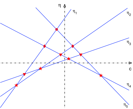
Figure 2: The functions $\eta_{j}(c)=k_{j}(k_{j}-c)$ for $(k_{1},k_{2},k_{3},k_{4},k_{5})=(-2,-1,-\frac{1}{2},\frac{3}{4},\frac{3}{2})$. The levels of intersection 0, 1, 2, 3 are respectively denoted by circles, diamonds, triangles and stars.

Let us now define a local coordinate frame $(\xi,y)$ in order to study the asymptotics for large $|y|$ with

$$x=c\,y+\xi\,.$$

Then the phase functions $\theta_{i}$ in $f$ of (1.6) become

$$\theta_{i}=-k_{i}\xi+\eta_{i}(c)\,y+\theta_{i}^{0}\,,\quad{\rm for}\quad i=1,\dots,N\,,$$

with

$$\eta_{i}(c):=k_{i}(k_{i}-c)\,.$$

Without loss of generality, we assume the ordering for the parameters $\{k_{i}\,|~{}i=1,\dots,N\}$,

$$k_{1}<k_{2}<\cdots<k_{N}\,.$$

Then one can easily show that the lines $\eta=\eta_{i}(c)$ are in general position; that is, each line $\eta=\eta_{i}(c)$ intersects with all other lines at $N-1$ distinct points in the $c$-$\eta$ plane; in other words, only two lines meets at each intersection point. Figure 2 shows a specific example, corresponding to the values $(k_{1},k_{2},k_{3},k_{4},k_{5})=(-2,-1,-\frac{1}{2},\frac{3}{4},\frac{3}{2})$.

Now the purpose is to find the dominant exponential terms in the $\tau_{{N_{+}}}$-function (2.3) for $y\to\pm\infty$ as a function of the velocity $c$. First note that if only one exponential is dominant, then $w_{1}=-\partial_{x}\log\tau_{{N_{+}}}$ is just a constant, and therefore the solution $u=-2\partial_{x}w_{1}$ is zero. Then, nontrivial contributions to $u$ arise when one can find two exponential terms which dominate over the others. Note that because the intersections of the $\eta_{i}$’s are always pairwise, three or more terms cannot make a dominant balance for large $|y|$. In the case of $({N_{-}},1)$-soliton solutions, it is easy to see that at each $c$ the dominant exponential term for $y\to\infty$ is provided by only $\eta_{1}$ and/or $\eta_{N}$, and therefore there is only one shock (${N_{+}}=1$) moving with velocity $c_{1,N}=k_{1}+k_{N}$ corresponding to the intersection point of $\eta_{1}$ and $\eta_{N}$ (see figure 2). On the other hand, as $y\to-\infty$, each term $\eta_{j}$ can become dominant for some $c$, and at each intersection point $\eta_{j}=\eta_{j+1}$ the two exponential terms corresponding to $\eta_{j}$ and $\eta_{j+1}$ give a dominant balance; therefore there are ${N_{-}}=N-1$ shocks moving with velocities $c_{j,j+1}=k_{j}+k_{j+1}$, for $j=1,\dots,N-1$ (see again figure 2).

In the general case, ${N_{+}}\neq 1$, the $\tau_{N_{+}}$-function in (2.3) involves exponential terms having combinations of phases, and two exponential terms that make a dominant balance can be found as follows: Let us first define the level of intersection of $\eta_{i}(c)$.

Definition 2.3.  Let $\eta_{i}(c)$ and $\eta_{j}(c)$ intersect at the value $c=c_{i,j}=k_{i}+k_{j}$, i.e., $\eta_{i}(c_{i,j})=\eta_{j}(c_{i,j})$. The level of intersection, denoted by $\sigma_{i,j}$, is defined as the number of other $\eta_{l}$’s that at $c=c_{i,j}$ are larger than $\eta_{i}(c_{i,j})=\eta_{j}(c_{i,j})$. That is,

$$\sigma_{i,j}:=\big{|}\{\eta_{l}\,|~{}\eta_{l}(c_{i,j})>\eta_{i}(c_{i,j})=\eta_{j}(c_{i,j})\}\big{|}\,.$$

We also define $I(n)$ as the set of pairs $(\eta_{i},\eta_{j})$ having the level $\sigma_{i,j}=n$, namely

$$I(n):=\{(\eta_{i},\eta_{j})\,|~{}\sigma_{i,j}=n,~{}{\rm for}~{}i<j\,\}.$$

The level of intersection can take the range $0\leq\sigma_{i,j}\leq N-2$. Then one can show:

Lemma 2.4.  The set $I(n)$ is given by

$$I(n)=\{(\eta_{i},\eta_{N-n+i-1})\,|~{}i=1,\dots,n+1\}\,.$$

Proof. From the assumption $k_{1}<k_{2}<\cdots<k_{N}$, we have the following inequality at $c=c_{i,j}$  (i.e. $\eta_{i}=\eta_{j}$) for $i<j$,

$$\eta_{i+1},\dots,\eta_{j-1}<\eta_{i}=\eta_{j}<\eta_{1},\dots,\eta_{i-1},\,\eta_{j+1},\dots,\eta_{N}\,.$$

Then taking $j=N-n-1$ leads to the assertion of the Lemma.        

Note here that the total number of pairs $(\eta_{i},\eta_{j})$ is

$$\left(\!\!\begin{array}[]{cc}N\\ 2\end{array}\!\!\right)={\textstyle\frac{1}{2}}N(N-1)=\mathop{\textstyle\sum}\limits_{n=0}^{N-2}|I(n)|\,.$$

We illustrate these definitions in figure 2, where the sets $I(n)$ for the level of intersection $n=0,1,2,3$, which are respectively marked by circles, diamonds, triangles and stars, are given by

$$\left\{\begin{array}[]{llll}I(0)=\{(\eta_{1},\eta_{5})\},\\[1.72218pt] I(1)=\{(\eta_{1},\eta_{4}),~{}(\eta_{2},\eta_{5})\},\\[1.72218pt] I(2)=\{(\eta_{1},\eta_{3}),~{}(\eta_{2},\eta_{4}),~{}(\eta_{3},\eta_{5})\},\\[1.72218pt] I(3)=\{(\eta_{1},\eta_{2}),~{}(\eta_{2},\eta_{3}),~{}(\eta_{3},\eta_{4}),~{}(\eta_{4},\eta_{5})\}.\end{array}\right.$$

For the case of $({N_{-}},{N_{+}})$-solitons, the following formulae are useful:

$$\left\{\begin{array}[]{ll}I({N_{-}}-1)=\{(\eta_{i},\eta_{{N_{+}}+i})\,|~{}i=1,\dots,{N_{-}}\}\,,\\[1.72218pt] I({N_{+}}-1)=\{(\eta_{i},\eta_{{N_{-}}+i})\,|~{}i=1,\dots,{N_{+}}\}\,.\end{array}\right.$$

Here recall that ${N_{+}}+{N_{-}}=N$. These formulae indicate that, for each intersecting pair $(\eta_{i},\eta_{j})$ with the level ${N_{-}}-1$ (${N_{+}}-1$), there are ${N_{+}}-1$ terms $\eta_{l}$’s which are smaller (larger) than $\eta_{i}=\eta_{j}$. Then the sum of those ${N_{+}}-1$ terms with either $\eta_{i}$ or $\eta_{j}$ provides two dominant exponents in the $\tau_{{N_{+}}}$-function for $y\to-\infty$ $(y\to\infty)$ (see more detail in the proof of Theorem 2). Note also that $|I(N_{\pm}-1)|=N_{\mp}$. Now we can state our main theorem:

Theorem 2.5.  Let  $w_{1}$  be a function defined by

$$w_{1}=-\frac{\partial}{\partial{x}}\log\tau_{N_{+}}\,,$$

with $\tau_{N_{+}}$ given by (2.3). Then  $w_{1}$  has the following asymptotics for $y\to\pm\infty:$

1. For  $y\to-\infty$  and  $x=c_{i,{N_{+}}+i}\,y+\xi$  for $i=1,\dots,{N_{-}}$ ,

   $$\kern 0.0ptw_{1}~{}\longrightarrow~{}\left\{\begin{array}[]{ll}K_{i}(-,-):=\mathop{\textstyle\sum}\limits_{j=i+1}^{{N_{+}}+i}k_{j}&\quad\mathrm{as}\quad\xi\to-\infty\,,\\ K_{i}(+,-):=\mathop{\textstyle\sum}\limits_{j=i}^{{N_{+}}+i-1}k_{j}&\quad\mathrm{as}\quad\xi\to\infty\,.\end{array}\right.$$

2. For  $y\to\infty$  and  $x=c_{i,{N_{-}}+i}\,y+\xi$  for $i=1,\dots,{N_{+}}$ ,

   $$\kern 0.0ptw_{1}~{}\longrightarrow~{}\left\{\begin{array}[]{ll}K_{i}(-,+):=\mathop{\textstyle\sum}\limits_{j=1}^{i-1}k_{j}+\mathop{\textstyle\sum}\limits_{j=1}^{{N_{+}}-i+1}k_{N-j+1}&\quad\mathrm{as}\quad\xi\to-\infty\,,\\ K_{i}(+,+):=\mathop{\textstyle\sum}\limits_{j=1}^{i}k_{j}+\mathop{\textstyle\sum}\limits_{j=1}^{{N_{+}}-1}k_{N-j+i}&\quad\mathrm{as}\quad\xi\to\infty\,.\end{array}\right.$$

where  $c_{i,j}=k_{i}+k_{j}$.

Proof. First note that at the point $\eta_{i}=\eta_{{N_{+}}+i}$, i.e., $(\eta_{i},\eta_{{N_{+}}+i})\in I({N_{-}}-1)$, from Lemma 2 we have the inequality,

$$\underbrace{\phantom{\bigg{|}}\kern-1.99997pt\eta_{i+1},\eta_{i+2},\dots,\eta_{i+{N_{+}}-1}}_{{N_{+}}-1}<\eta_{i}=\eta_{{N_{+}}+i}\,.$$

This implies that, for $c=k_{i}+k_{{N_{+}}+i}$, the following two exponential terms in the $\tau_{N_{+}}$-function in Lemma 2,

$$\exp\bigg{(}\mathop{\textstyle\sum}\limits_{j=i}^{{N_{+}}+i-1}\theta_{j}\bigg{)}\,,\qquad\exp\bigg{(}\mathop{\textstyle\sum}\limits_{j=i+1}^{{N_{+}}+i}\theta_{j}\bigg{)}\,,$$

provide the dominant terms for $y\to-\infty$. Note that the condition $\eta_{i}=\eta_{{N_{+}}+i}$ leads to $c=c_{i,{N_{+}}+i}=k_{i}+k_{{N_{+}}+i}$. Thus the function $w_{1}$ can be approximated by the following form along $x=c_{i,{N_{+}}+i}\,y+\xi$ for $y\to-\infty$:

$$\kern-5.0pt\begin{array}[]{llll}w_{1}&\sim&\displaystyle-\frac{\partial}{\partial{\xi}}\log\big{(}\Delta_{i}(+,-)e^{-K_{i}(+,-)\xi}+\Delta_{i}(-,-)e^{-K_{i}(-,-)\xi}\big{)}\\[6.88889pt] &=&\displaystyle{\frac{K_{i}(+,-)\Delta_{i}(+,-)e^{-K_{i}(+,-)\xi}+K_{i}(-,-)\Delta_{i}(-,-)e^{-K_{i}(-,-)\xi}}{\Delta_{i}(+,-)e^{-K_{i}(+,-)\xi}+\Delta_{i}(-,-)e^{-K_{i}(-,-)\xi}}\,,}\\[6.88889pt] &=&\displaystyle{\frac{K_{i}(+,-)\Delta_{i}(+,-)e^{(k_{{N_{+}}+i}-k_{i})\xi}+K_{i}(-,-)\Delta_{i}(-,-)}{\Delta_{i}(+,-)e^{(k_{{N_{+}}+i}-k_{i})\xi}+\Delta_{i}(-,-)}\,,}\end{array}$$

where

$$\Delta_{i}(+,-)=\Delta(i,\dots,{N_{+}}+i-1)\,\,\exp\bigg{(}\mathop{\textstyle\sum}\limits_{j=i}^{{N_{+}}+i-1}\theta_{j}^{0}\bigg{)}$$

$$\Delta_{i}(-,-)=\Delta(i+1,\dots,{N_{+}}+i)\,\,\exp\bigg{(}\mathop{\textstyle\sum}\limits_{j=i+1}^{{N_{+}}+i}\theta_{j}^{0}\bigg{)}\,.$$

Now, from $k_{i}<k_{{N_{+}}+i}$ it is obvious that $w_{1}$ has the desired asymptotics as $\xi\to\pm\infty$ for $y\to-\infty$.

Similarly, for the case of $(\eta_{i},\eta_{{N_{-}}+i})\in I({N_{+}}-1)$ we have the inequality

$$\eta_{i}=\eta_{{N_{-}}+i}<\underbrace{\phantom{\bigg{|}}\kern-1.99997pt\eta_{1},\eta_{2},\dots,\eta_{i-1},\eta_{{N_{-}}+i+1}\dots,\eta_{N}}_{{N_{+}}-1}\,.$$

Then the dominant terms in the $\tau_{N_{+}}$-function on $x=c_{i,{N_{-}}+i}y+\xi$ for $y\to\infty$ are given by the exponential terms

$$\exp\bigg{(}\mathop{\textstyle\sum}\limits_{j=1}^{i}\,\theta_{j}~{}+\mathop{\textstyle\sum}\limits_{j=1}^{{N_{+}}-i}\,\theta_{N-j+1}\bigg{)}\,,\qquad\exp\bigg{(}\mathop{\textstyle\sum}\limits_{j=1}^{i-1}\,\theta_{j}~{}+\mathop{\textstyle\sum}\limits_{j=1}^{{N_{+}}-i+1}\,\theta_{N-j+1}\bigg{)}\,.$$

Then, following the previous argument, we obtain the desired asymptotics as $\xi\to\pm\infty$ for $y\to\infty$.

For other values of $c$, that is for $c\neq c_{i,{N_{+}}+i}$ and $c\neq c_{i,{N_{-}}+i}$, just one exponential term becomes dominant, and thus $w_{1}$ approaches a constant as $|y|\to\infty$. This completes the proof.          

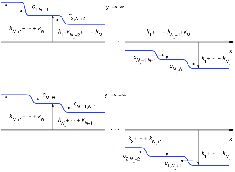
Figure 3: Asymptotic behavior of the function $w_{1}$ with $k_{1}<k_{2}<\cdots\leq 0<\cdots<k_{N-1}<k_{N}$. As $y\to-\infty$ there are ${N_{-}}$ jumps, moving with velocities $c_{j,{N_{+}}+j}$ ($j=1,\dots,{N_{-}}$). As $y\to\infty$ there are ${N_{+}}$ jumps, moving with velocities $c_{i,{N_{-}}+i}$ ($i=1,\dots,{N_{+}}$).

Theorem 2 can be summarized in figure 3: As $y\to-\infty$, the function $w_{1}$ has ${N_{-}}$ jumps, moving with velocities $c_{j,{N_{+}}+j}$ for $j=1,\dots,{N_{-}}$; as $y\to\infty$, $w_{1}$ has ${N_{+}}$ jumps, moving with velocities $c_{i,{N_{-}}+i}$ for $i=1,\dots,{N_{+}}$. Each jump represents a line soliton of the $u$-solution, and therefore the whole solution represents an $({N_{-}},{N_{+}})$-soliton. Each velocity of the asymptotic line solitons in the $({N_{-}},{N_{+}})$-soliton is determined from the $c$-$\eta$ graph of the levels of intersections (see figure 2). For example, in the case of $(1,4)$-soliton in figure 2, one incoming soliton has velocity $c_{1,4+1}=c_{1,5}$, corresponding to the set $I(0)$, and four outgoing solitons have the velocities $c_{i,1+i}$ for $i=1,\dots,4$, corresponding to $I(3)$. Note that, given a set of $N$ phases (as determined by the parameters $k_{i}$ for $i=1,\dots,N$), the same graph can be used for any $({N_{-}},{N_{+}})$-soliton with ${N_{-}}+{N_{+}}=N$. In particular, if $N=2M$, we have ${N_{+}}={N_{-}}=M$, and Theorem 2 implies that the velocities of the $M$ incoming solitons are equal to those of the $M$ outgoing solitons. However, we show in the next section that these (resonant) $M$-soliton solutions are different from the ordinary (nonresonant) multi-soliton solutions of the KP equation.

We remark that Theorem 2 determines the complete structure of asymptotic patterns of the solutions $u(x,y,t)$ given by (1.2) for the Toda lattice equation. In the case of the ordinary multi-soliton solution of the KP equation, the tau-function (1.3) does not contain all the possible combinations of phases, and therefore the theorem should be modified. However, the key idea for the asymptotic analysis of using the levels of intersection is still applicable. In fact, one can find from the same argument that the asymptotic velocities for the ordinary $M$-solitons are given by $c_{2i-1,2i}=k_{2i-1}+k_{2i}$ where the $\tau_{M}$-function is the Wronskian (1.3) with $f_{i}=e^{\theta_{2i-1}}+e^{\theta_{2i}}$ for $i=1,\dots,M$ and $k_{1}<k_{2}<\cdots<k_{2M}$. Note that the velocities are different from those of the resonant $M$-soliton solution for the Toda case.

Finally, it should be noted that the asymptotic values $w_{1,j}:=-\partial_{x}\log\tau_{j}$ as $\xi\to\pm\infty$ show the sorting property of the Toda lattice equation; that is, for $j=1,\dots,N$,

$$b_{j}=\frac{\partial}{\partial{x}}\log\frac{\tau_{j}}{\tau_{j-1}}=w_{1,j-1}-w_{1,j}~{}\longrightarrow~{}\left\{\begin{array}[]{ll}-k_{j}&\quad\mathrm{as}\quad\xi\to\infty\,,\\ -k_{N-j+1}&\quad\mathrm{as}\quad\xi\to-\infty\,.\end{array}\right.$$

Also, one can easily show that $a_{j}\to 0$ as $|\xi|\to\infty$, which implies the sorting behavior, i.e.,

$$L~{}\longrightarrow~{}\left\{\begin{array}[]{ll}\mathop{\rm diag}\nolimits(-k_{1},-k_{2},\dots,-k_{N})&\quad\mathrm{as}\quad\xi\to\infty\,,\\ \mathop{\rm diag}\nolimits(-k_{N},-k_{N-1},\dots,-k_{1})&\quad\mathrm{as}\quad\xi\to-\infty\,.\end{array}\right.$$

Recall here that the set $\{\lambda=-k_{i}\,|~{}i=1,\dots,N\}$ contains the eigenvalues of the Lax matrix $L$, with $\lambda_{1}>\cdots>\lambda_{N}$ as mentioned in (1.12).

3 Intermediate patterns of soliton interactions

In this section we describe the intermediate patterns of the resonant solitons in the $x$-$y$ plane. The key idea is to consider the pattern as a collection of fundamental resonances. The fundamental resonance consists of three parameters: $\{k_{1},k_{2},k_{3}\}$, that is, the case of $N=3$ with $|{N_{-}}-{N_{+}}|=1$. Without loss of generality, let us take ${N_{-}}=1$ and ${N_{+}}=2$, i.e., a (1,2)-soliton. (The case of a (2,1)-soliton is obtained from the symmetry $(x,y,t)\to(-x,-y,-t)$ of the KP equation, i.e., from the duality of the determinants, $\tau_{1}$ and $\tau_{2}$ for $N=3$.)  Then, with $k_{1}<k_{2}<k_{3}$, the pattern of the fundamental resonance is a Y-shape graph as shown in figure 4. Here and in the following we denote with $[i,j]$ the asymptotic line soliton with $c=c_{i,j}=k_{i}+k_{j}$. Notice that $I({N_{-}}-1)=I(0)=\{(\eta_{1},\eta_{3})\}$ and $I({N_{+}}-1)=I(1)=\{(\eta_{1},\eta_{2}),(\eta_{2},\eta_{3})\}$.

One should note that at the vertex of the Y-shape graph each index appears exactly twice as the result of resonance, and in figure 4b those vertices form a triangle, which we refer to as a “resonant triangle”. The resonant triangle is equivalent to the resonance condition for the wavenumber vectors in (2.2). Since the vertex of the Y-shape graph consists of three line solitons, $\theta_{i}=\theta_{j},~{}1\leq i<j\leq 3$, the location of the vertex is obtained from the solution of the equations $\theta_{1}=\theta_{2}=\theta_{3}$, i.e.,

$$\left(\!\begin{array}[]{cc}k_{1}-k_{2}&-(k_{1}^{2}-k_{2}^{2})\\ k_{1}-k_{3}&-(k_{1}^{2}-k_{3}^{2})\end{array}\!\right)\left(\!\!\begin{array}[]{c}x\\ y\end{array}\!\!\right)=\left(\!\!\begin{array}[]{c}\theta_{1}^{0}-\theta_{2}^{0}-(k_{1}^{3}-k_{2}^{3})t\\ \theta_{1}^{0}-\theta_{3}^{0}-(k_{1}^{3}-k_{3}^{3})t\end{array}\!\!\right)\,.$$

Note here that the coefficient matrix is nonsingular for $k_{1}<k_{2}<k_{3}$, and the location $(x,y)$ is uniquely determined by a function of $t$. This implies that there always exists a Y-shape graph if there are three line solitons satisfying the resonance conditions (2.2). Since the $\tau_{{N_{+}}}$-function (2.3) contains all possible combinations of ${N_{+}}$ phases, all the vertices in the graph form Y-shape intersections as a result of dominant balance of three exponential terms in the $\tau_{{N_{+}}}$ at each vertex. One should also note that a vertex with 4 or more line solitons is not generic: A vertex with $m$ distinct line solitons is obtained from the system of $m$ equations, $\{\theta_{i_{k}}=\theta_{j_{k}}~{}|~{}i_{k}\neq j_{k},~{}k=1,\dots,m\}$, in which at least $m-1$ equations are linearly independent. Then for $m\geq 4$, this system in $(x,y)$ is overdetermined, so that the solution exists only for specific choices of $\theta_{i}^{0}$ for fixed values of $t$. In the cases of both ordinary and resonant 2-soliton solutions, the two pairs of solitons as $y\to\pm\infty$ are the same, and therefore there are only two independent equations. Also, as mentioned before, the ordinary 2-soliton solution needs a balance of four exponential terms to realize an X-shape vertex. However, this balance cannot be dominant over a balance of three terms with the $\tau_{{N_{+}}}$-function given by (2.3). In what follows, we show that the X-shape vertex of an ordinary 2-soliton solution is blown up into a hole with four Y-shape vertices for the resonant 2-soliton solution.

 

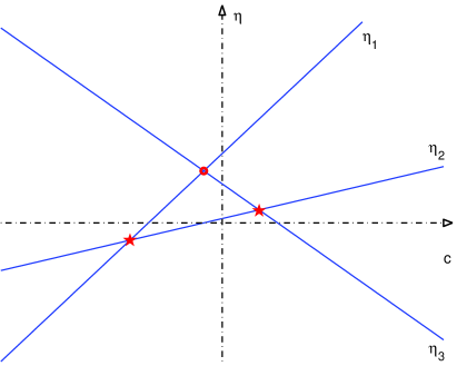
Figure 4: The Y-shape graph (left) illustrating a fundamental resonance with $(k_{1},k_{2},k_{3})=(-1,-\frac{1}{4},\frac{3}{4})$ and the corresponding functions $\eta_{i}(c)$, $i=1,2,3$ (right). The graph to the left represents contour lines of $u(x,y,t)$. The circle at the level set $I(0)$ corresponds to the incoming soliton, and the stars at $I(1)$ correspond to the outgoing solitons.

We now consider the case with ${N_{-}}=2$ and ${N_{+}}=2$, which describes the resonant 2-soliton solution. We can start with the graph in figure 4 having $k_{1}<k_{2}<k_{3}$. Then we add $k_{4}$ with $k_{3}<k_{4}$. From Theorem 2 we find that both asymptotic solutions for $y\to\pm\infty$ consist of the solitons with [1,3] and [2,4]. With $k_{1}<k_{2}<k_{3}<k_{4}$, the velocity $c_{2,4}$ of the additional soliton [2,4] as $y\to-\infty$ satisfies $c_{2,4}>c_{2,3}>c_{1,2}$. For sufficiently large negative values of $t$, the [2,4] soliton starts in the left side of the [1,3] soliton and first intersects with the [1,2] soliton; then the resonance condition determines that the [1,2] and [2,4] solitons merge and make a new outgoing soliton [1,4]. Since the ${N_{+}}$ solitons consist of [1,3] and [2,4], this [1,4] soliton first branches to [1,3] and [3,4]. Then the intermediate [3,4] soliton now intersects with the [2,3] soliton to form the [2,4] outgoing soliton. (Note that $c_{3,4}$ is the largest velocity among these solitons.) The process forming a resonant 2-soliton is shown in figure 5. Note here that there are four vertices in the interaction pattern, which correspond to the four resonant triangles in the $c$-$\eta$ plane.

 

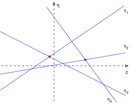
Figure 5: A resonant 2-soliton solution $u(x,y,t)$ (left) with $(k_{1},k_{2},k_{3},k_{4})=(-1,-\frac{1}{4},\frac{3}{4},2)$ and the corresponding functions $\eta_{i}(c)$ (right). Both incoming and outgoing solitons correspond to the interstections marked by circles at the level set $I(1)$.

One should also note that the [2,4] soliton cannot intersect directly the [1,3] soliton unless a [1,2] soliton or a [3,4] soliton are created as intermediate solitons. The graph of this latter case is obtained from figure 5 by letting $(x,y,t)\to(-x,-y,-t)$. Also note that the ordinary 2-soliton solution with those same parameters $(k_{1},\dots,k_{4})$ for $\{f_{1},f_{2}\}$ in (1.4) has different asymptotic solitons, namely [1,2] and [3,4], and, because of the missing exponential terms in the $\tau_{2}$-function, this ordinary 2-soliton solution cannot have resonant interactions; that is, no resonant triangle can be formed with only those exponential terms. This is also true for any ordinary multi-soliton solutions of the KP equation.

We can continue the process of adding $n$ new incoming solitons to the graph in figure 5 to get a $(2+n,2)$-soliton solution. One can also add $m$ new outgoing solitons to the new graph to obtain a $(2+n,2+m)$-soliton solution. This last step can be done by adding $m$ incoming solutions to a $(2,2+n)$-soliton solution, which is simply obtained by the $\pi$ rotation (i.e., $(x,y)\to(-x,-y)$) of the graph of the $(2+n,2)$-solution using the duality of the determinant. Then one can show the following:

Proposition 3.1.  In the generic situation, the number of holes (bounded regions) in the graph of the $({N_{-}},{N_{+}})$-soliton solution is $({N_{-}}-1)({N_{+}}-1)$.

Proof. We use mathematical induction. The case ${N_{+}}=1$ corresponds to the Burgers equation, and it is immediate to show that the graph of the ($N_{-}$,1)-soliton solution has a tree shape; that is, no holes (see also Ref. [10]). Now suppose that the $({N_{-}},{N_{+}})$-soliton has $({N_{-}}-1)({N_{+}}-1)$ holes. Add a new phase $\theta_{N+1}$, with $k_{N+1}$ satisfying $k_{1}<\cdots<k_{N}<k_{N+1}$, which produces a new, fastest, incoming $[{N_{-}}+1,N+1]$ soliton, and assume that this solution intersects with the $[1,{N_{-}}+1]$ soliton, which is the slowest outgoing soliton. Then the resonant process of those solitons generates a $[1,N+1]$-soliton as a (2,1) process, which then intersects with the new slowest $[1,N+2]$ soliton to generate an intermediate $[{N_{-}}+2,N+1]$ soliton. This intermediate soliton interacts with the second slowest outgoing soliton, the $[2,N+2]$ soliton, to generate $[2,N+3]$ and $[N+3,N+1]$ solitons, and so on. This process is illustrated in figure 6. From this figure, it is obvious that there are ${N_{+}}-1$ newly created holes; that is, if $({N_{-}},{N_{+}})\to({N_{-}}+1,{N_{+}})$, the number of holes increases as

$$({N_{-}}-1)({N_{+}}-1)\to({N_{-}}-1)({N_{+}}-1)+({N_{+}}-1)={N_{-}}({N_{+}}-1)\,.$$

The case of the $({N_{-}},{N_{+}}+1)$ solution can be analyzed in the same way using the duality of the determinants. This completes the proof.        

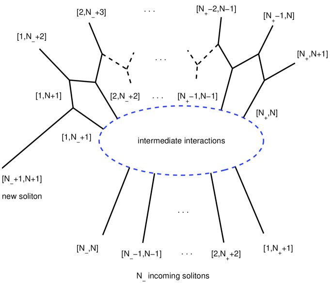
Figure 6: A schematic diagram illustrating the creation of new holes in the resonant interaction process for a $({N_{-}}+1,{N_{+}})$-soliton solution with ${N_{-}}+{N_{+}}=N$. The new soliton $[{N_{-}}+1,N+1]$ is assumed to have a resonant interaction with the previous outgoing soliton $[1,{N_{-}}+1]$.

One can also show the following from Proposition 3:

Corollary 3.2.  In the generic situation for ${N_{-}}+{N_{+}}=N\geq 3$, the total numbers of intersection points and intermediate solitons in a $({N_{-}},{N_{+}})$-soliton solution are respectively given by  $2{N_{-}}{N_{+}}-N$  and  $3{N_{-}}{N_{+}}-2N$.

Proof. By applying mathematical induction on figure 6, one can easily find that the number of new vertices (intersection points) is $2{N_{+}}-1$ and that of new intermediate solitons is $3{N_{+}}-2$. This yields the desired results.        

One should compare these numbers with the case of ordinary $M$-soliton solution, where the total numbers of holes and intersection points are ${\textstyle\frac{1}{2}}(M-1)(M-2)$ and ${\textstyle\frac{1}{2}}M(M-1)$, respectively. The resonant process blows up each vertex in an ordinary $M$-soliton solution to create a hole, so that the total number of holes in a resonant $M$-soliton solution is given by

$${\textstyle\frac{1}{2}}(M-1)(M-2)+{\textstyle\frac{1}{2}}M(M-1)=(M-1)^{2}\,.$$

Note also that the total number of vertices in a resonant $M$-soliton is four times of the vertices of an ordinary $M$-soliton, i.e. each vertex is blown up to make 4 vertices with one hole.

  (a)     (b) 

 

  (c)     (d) 

 

Figure 7: Snapshots illustrating the temporal evolution of a resonant 3-soliton solution $u(x,y,t)$ with $(k_{1},\dots,k_{6})=(-\frac{5}{2},-\frac{5}{4},-\frac{1}{2},\frac{1}{2},\frac{3}{2},\frac{5}{2})$ and $\theta_{1}^{0}=\cdots=\theta_{6}^{0}=0$: (a) $t=-10$, (b) $t=0$, (c) $t=10$, (d) $t=20$. Note the symmetry $(x,y,t)\leftrightarrow(-x,-y,-t)$ in (a) and (c).

  (a)     (b) 

 

  (c)     (d) 

 

Figure 8: Snapshots illustrating the temporal evolution of a (4,3)-soliton solution $u(x,y,t)$ with $(k_{1},\dots,k_{7})=(-3,-2,-1,0,1,2,3)$ and $\theta_{1}^{0}=\cdots=\theta_{7}^{0}=0$: (a) $t=-8$, (b) $t=0$, (c) $t=8$, (d) $t=16$. Note the symmetry $(x,y,t)\leftrightarrow(-x,y,-t)$ in (a) and (c).

Figure 7 shows a few snapshots illustrating the temporal evolution of a resonant 3-soliton solution with $(k_{1},\dots,k_{6})=(-\frac{5}{2},-\frac{5}{4},-\frac{1}{2},\frac{1}{2},\frac{3}{2},\frac{5}{2})$. This resonant 3-soliton is similar to the “spider-web-like” soliton solution found for the cKP equation (cf. figure 10 in Ref. [9]), even though the underlying equation is different in those two cases. As described in this paper, the behavior is determined by the structure of the tau-function which is just the sum of exponential functions. The tau-functions of the KP and cKP equations have the same structure for those solutions.

Figure 8 shows the temporal evolution of a (4,3)-soliton solution with $(k_{1},\dots,k_{7})=(-3,-2,-1,0,1,2,3)$. In both figure 7 and figure 8, it can be observed that different intermediate solitons mediate the interaction process at different times. Also note that, for some finite values of $t$, the number of holes in the solution changes. However, Proposition 3 applies in the generic situation, and the total number of holes remains $({N_{-}}-1)({N_{+}}-1)$, namely 4 holes in figure 7 and 6 holes in figure 8. In both figures, we have set all $\theta_{i}^{0}=0$, so that all line solitons merge initially at the origin. It should be noted that even though several solitons might merge at the same point for some finite values of $t$, generically the resonant interactions are always among three solitons, i.e., fundamental resonances, as explained in this paper.

Finally, we would like to point out that the KP equation has a large variety of multi-soliton-type solutions. Among those solutions, we found that, since the $\tau_{{N_{+}}}$-function of the resonant $({N_{-}},{N_{+}})$-soliton for the Toda lattice hierarchy contains all possible combinations of phase terms $\{\theta_{i}\,|~{}i=1,\dots,N\}$, the interaction process for these solutions results in a fully resonant situation. On the other hand, the ordinary $M$-soliton solutions display a nonresonant case; that is, resonant triangles representing either (2,1)- or (1,2)-solitons cannot be formed because of the missing exponential terms in the tau-function. One can then find a partially resonant case consisting of ordinary multi-soliton interaction with the addition of some resonant interactions; one such example is the case having $f_{1}=e^{\theta_{1}}+e^{\theta_{2}}+e^{\theta_{3}}$ and $f_{2}=\rme^{\theta_{3}}+e^{\theta_{4}}$ for the $\tau_{2}$-function (1.3) where the ordinary 2-soliton interaction coexists with resonant interactions. We will report the details of the general patterns for multi-soliton-like solutions for the KP equation in a future communication.

Appendix: The Wronskian solutions of the KP hierarchy

In this Appendix we briefly explain how the Wronskian solution (1.3) is obtained from the Sato theory (see Ref. [14] for more details). The Sato theory is formulated on the basis of a pseudo-differential operator,

$${\mathcal{L}}=\partial+u_{2}\partial^{-1}+u_{3}\partial^{-2}+\cdots,$$

where $\partial$ is a derivation satisfying $\partial\,\partial^{-1}=\partial^{-1}\,\partial=1$ and the generalized Leibnitz rule,

$$\partial^{\nu}(fg)=\mathop{\textstyle\sum}\limits_{k=0}^{\infty}\bigg{(}\!\!\begin{array}[]{cc}\nu\\ k\end{array}\!\!\bigg{)}\,\frac{\partial^{k}f}{\partial x^{k}}\,\,\partial^{\nu-k}g\,,\qquad\mathrm{for}\quad\nu\in{\mathbb{Z}}\,.$$

(Note that the series terminates if and only if $\nu$ is a positive integer.) Then the KP hierarchy can be written in the Lax form

$$\frac{\partial{\mathcal{L}}}{\partial t_{n}}=[{\mathcal{B}}_{n},{\mathcal{L}}],\quad\mathrm{with}\quad{\mathcal{B}}_{n}:=({\mathcal{L}}^{n})_{\geq 0},$$ (A.1)

where $({\mathcal{L}}^{n})_{\geq 0}$ represents the polynomial (differential) part of ${\mathcal{L}}^{n}$ in $\partial$. Here the solution of the KP equation (1) is given by $u=2u_{2}$ with $t_{1}=x,~{}t_{2}=y$ and $t_{3}=t$.

Now writing ${\mathcal{L}}$ in the dressing form,

$${\mathcal{L}}={\mathcal{W}}{\partial}{\mathcal{W}}^{-1},\quad{\rm with}\quad{\mathcal{W}}=1+w_{1}\partial^{-1}+w_{2}\partial^{-2}+\cdots,$$

the KP hierarchy becomes

$$\frac{\partial{\mathcal{W}}}{\partial t_{n}}={\mathcal{B}}_{n}{\mathcal{W}}-{\mathcal{W}}\,\partial^{n}.$$ (A.2)

Using (A.1), the variables $u_{i}$’s can be expressed in terms of $w_{j}$’s; for example,

$$\left\{\begin{array}[]{ll}u_{2}=-w_{1,x},\\[1.72218pt] u_{3}=-w_{2,x}+w_{1}w_{1,x},\end{array}\right.$$

and so on. (Here and in the following, subscripts $x$ and $t_{n}$ denote partial differentiation.)  The equations for $w_{j}$ are, for example,

$$\left\{\begin{array}[]{ll}w_{1,t_{2}}=-2w_{1}w_{1,x}+w_{1,xx}+2w_{2,x},\\[1.72218pt] w_{2,t_{2}}=-2w_{2}w_{1,x}+w_{2,xx}+2w_{3,x},\end{array}\right.$$

and so on. Here one can easily show that a finite truncation of ${\mathcal{W}}$, given by

$${\mathcal{W}}_{M}:=1+w_{1}\partial^{-1}+\cdots+w_{M}\partial^{-M}\,,$$

is invariant under the equation (A.2). For example, the ${\mathcal{W}}$-equation with $M=1$ truncation, i.e. ${\mathcal{W}}_{1}=1+w_{1}\partial^{-1}$, is just the Burgers equation,

$$w_{1,t_{2}}=-2w_{1}w_{1,x}+w_{1,xx}.$$ (A.3)

For the $M$-truncation, consider the ordinary differential equation for a function $f$,

$${\mathcal{W}}_{M}\partial^{M}f=f^{(M)}+w_{1}f^{(M-1)}+\cdots+w_{M}f=0.$$ (A.4)

Let $\{f_{j}\,|~{}j=1,\dots,M\}$ be a fundamental set of solutions of (A.4). Then the coefficient function $w_{1}$ is expressed in terms of the Wronskian for the set of those solutions, i.e.,

$$w_{1}=-\frac{\partial}{\partial x}\log\tau_{M}\,,\qquad{\rm with}\quad\tau_{M}={\rm Wr}(f_{1},\dots,f_{M}).$$

which leads to a solution of the KP equation,

$${u=2u_{2}=-2\frac{\partial}{\partial x}w_{1}=2\frac{\partial^{2}}{\partial x^{2}}\log\tau_{M}\,.}$$

Recall that for $M=1$ this equation gives the well-known Cole-Hopf transformation between the Burgers equation for $w_{1}$ and the linear diffusion equation for $\tau_{1}=f$. One can also show from (A.2) that $f$ satisfies the linear partial differential equations,

$$\frac{\partial f}{\partial t_{n}}=\frac{\partial^{n}f}{\partial x^{n}},\quad{\rm for}\quad n=1,2,\dots.$$

Thus the equations for $(w_{1},\dots,w_{M})$ on the $M$-truncation are linearizable, and the behavior of the solutions is expected to be similar to the case of the Burgers equation. (The $M$-truncated equation is a multi-component extension of the Burgers equation [6].) This is one of the main motivations of the present study.

References

References

• [1] Adler M and van Moerbeke P 1994 J. Phys. A: Math. Gen.Adv. in Math. &108, 140–204
• [2] Casian L and Kodama Y 2002 J. Phys. A: Math. Gen.Contemp. Math. 301, 283–310
• [3] Flaschka H 1974 J. Phys. A: Math. Gen.Prog. Theor. Phys. 51, 703–716
• [4] Freeman N C and Nimmo J J C 1983 J. Phys. A: Math. Gen.Phys. Lett. 95A, 1–3
• [5] Gantmacher F R 1959 Theory of Matrices Vol. 2, (Chelsea, New York)
• [6] Harada H 1987 , J. Phys. A: Math. Gen.J. Phys. Soc. Japan 56, 3847–3852
• [7] Hirota R 1976 , in Bäcklund transformations, Miura R M Ed., Lecture Notes in Mathematics, 515 (Springer-Verlag, New York)
• [8] Hirota R, Ohta Y and Satsuma J 1988 J. Phys. A: Math. Gen.Prog. Theor. Phys. Suppl. 94, 59–72
• [9] Isojima S, Willox R and Satsuma J 2002 , J. Phys. A: Math. Gen.J. Phys. A, Math. Gen. 35, 6893–6909
• [10] Medina E 2002 J. Phys. A: Math. Gen.Lett. Math. Phys. 62, 91–99
• [11] Miles J W 1977 , J. Phys. A: Math. Gen.J. Fluid Mech. 79, 171–179
• [12] Moser J 1975 , J. Phys. A: Math. Gen.Springer Lecture Notes in Mathematics 38, 467–497
• [13] Nakamura Y and Kodama Y 1995 J. Phys. A: Math. Gen.Acta Appl. Math. 39, 435–443
• [14] Ohta Y, Satsuma J, Takahashi D and Tokihiro T 1988 , J. Phys. A: Math. Gen.Prog. Theor. Phys. Suppl. 94, 210–241
• [15] Whitham G B 1974 Linear and nonlinear waves (Wiley, New York), 110–112