Stochastic Stabilization of Cosmological Photons

The stability of photon trajectories in models of the Universe that have constant spatial curvature is determined by the sign of the curvature: they are exponentially unstable if the curvature is negative and stable if it is positive or zero. We demonstrate that random fluctuations in the curvature provide an additional stabilizing mechanism. This mechanism is analogous to the one responsible for stabilizing the stochastic Kapitsa pendulum. When the mean curvature is negative it is capable of stabilizing the photon trajectories; when the mean curvature is zero or positive it determines the characteristic frequency with which neighbouring trajectories oscillate about each other. In constant negative curvature models of the Universe that have compact topology, exponential instability implies chaos (e.g. mixing) in the photon dynamics. We discuss some consequences of stochastic stabilization in this context.

One of the fundamental questions concerning the dynamical properties of photons in the Universe is whether their trajectories are stable or unstable. This strongly influences both the images of distant objects as well as fluctuations in the cosmic microwave background (CMB). In cosmological models in which the spatial geometry of the Universe has constant curvature $K$ the photon trajectories (geodesics) are stable if $K>0$, in which case neighbouring trajectories oscillate about each other with a characteristic frequency determined by $K$, and exponentially unstable if $K<0$, in which case neighbouring trajectories diverge exponentially quickly with a Liapunov exponent determined by $|K|$.

It is obvious, however, that the Universe is not exactly homogeneous and isotropic: matter is not uniformly distributed but is organized into galaxies, clusters of galaxies, and even superclusters of galaxies [2]. Consequently, the spatial curvature cannot be constant, but fluctuates. Our purpose here is to investigate the influence of these fluctuations on the stability of the photon trajectories. It might be thought that random fluctuations in the curvature would be a source of instability. We show that this is not in fact the case; their influence is a stabilizing one in that the curvature is renormalized by an additional (positive) factor related to the fluctuation amplitude and length-scales. The mechanism responsible for this stochastic stabilization is analogous to the one that stabilizes the Kapitsa pendulum: a pendulum whose pivot is forced to move periodically or stochastically along the vertical [3].

Given the fact that for constant curvature models to be consistent with recent observations of the CMB the absolute value of the mean curvature must be small – the density of energy in the Universe is within about $1\%$ of its critical value [4] – stochastic stabilization is capable of dominating the stability balance. For example, an order of magnitude estimate suggests that it is relevant in the present cosmological epoch. The difference between a constant curvature model with $K$ close to zero and one in which stochastic stabilization dominates is quantifiable in terms of the stability frequency with which neighbouring trajectories oscillate about each other.

Our results apply to both open and compact geometries. There has, however, recently been considerable attention focused on negative curvature models that have compact topology [5, 6, 7, 8, 9, 10, 11]. Photon dynamics in compact spaces is recurrent and hence, by virtue of the exponential instability, strongly chaotic (e.g. mixing) when the curvature is constant and negative. The fact that fluctuations in the cosmic microwave background (CMB) have a distribution close to gaussian has been related to Berry’s random wave model [12] for wave modes in chaotic systems [8, 11] and the phenomenon of scarring in these wave modes [13] has been linked with anisotropic structures in the CMB and in the distribution of galaxies [8, 11]. We discuss some implications of stochastic stabilization in this context.

We begin by deriving the appropriate form of the geodesic deviation equation – the equation that governs the separation of neighbouring trajectories. Since the aim of this Letter is to establish the principle of stochastic stabilization for photon trajectories, the calculations we report contain the essential ingredients for the effect, but ignore many additional, comparatively weaker phenomena present in the early Universe. With this in mind, we begin with an expanding isotropic homogeneous (Friedmann) cosmology perturbed by density fluctuations with non-relativistic velocities, neglecting perturbations of vector and tensor character such as gravitational waves, and pressure fluctuations, for example caused by relativistic neutrinos. In the coordinate system called the ‘conformal Newtonian’ or ‘longitudinal’ gauge [14], with the spatial variables in Robertson-Walker form, such a spacetime is described by the metric

$$ds^{2}=R^{2}(\tau)\{(1+2\Phi)d\tau^{2}-\frac{1-2\Phi}{[1+\frac{K}{4}(x^{2}+y^{2}+z^{2})]^{2}}(dx^{2}+dy^{2}+dz^{2})\}.$$ (1)

Here $R(\tau)$ is the scale factor or spatial curvature radius of the Universe, $\tau=\int R^{-1}dt$ is conformal time, $\Phi<<1$ is the Newtonian gravitational potential, $K$ is the dimensionless spatial curvature (e.g. $K=-1$ corresponds to a hyperbolic geometry), $(x,y,z)$ are comoving coordinates expanding at the same rate as the Universe, and units are chosen in which Newton’s constant $G$ and the speed of light $c$ are equal to unity. The paths of photons through the spacetime are null geodesics described by the equation [15]

$$\frac{d{\bf n}}{d\tau}=-2\nabla_{\perp}\Phi$$ (2)

where $\bf n$ is the photon direction, and $\nabla_{\perp}$ is the gradient in comoving coordinates perpendicular to $\bf n$. Note that since $\Phi$ and its derivative are small, the total change of $\bf n$ is small, and so the transverse derivative can be replaced by the derivative transverse to the observed (final) direction of the photon. The separation of two closely spaced photons propagates according to the geodesic deviation equation [16] which under our approximations leads to

$$\frac{d^{2}}{d\tau^{2}}\begin{pmatrix}\xi\\ \eta\end{pmatrix}=-\begin{pmatrix}K+2\Phi_{\xi\xi}&2\Phi_{\xi\eta}\\ 2\Phi_{\xi\eta}&K+2\Phi_{\eta\eta}\end{pmatrix}\begin{pmatrix}\xi\\ \eta\end{pmatrix}$$ (3)

where $\xi$ and $\eta$ are the components of the separations orthogonal to $\bf n$, and there are contributions arising from both the spatial curvature $K$ and second derivatives of the gravitational potential in directions orthogonal to $\bf n$, namely tidal forces.

These tidal forces are, in principle, entirely characterized by a complete knowledge of the fluctuations in the matter density. We shall consider them to be random functions of position (and possibly time). As it moves under their influence, a photon will be seen to be acted on by a time-varying force which fluctuates rapidly (because the speed of light is large and the length scale of the density fluctuations is small compared to $R$) and randomly (i.e. stochastically) with zero mean. We thus replace the spatially random tidal force terms in (3) with a time-dependent stochastic perturbation.

In order to illustrate the qualitative behaviour of the solutions of the resulting class of equations, we consider first the analogous one-component case:

$$\frac{d^{2}u}{d\tau^{2}}=-(k+Af(\tau))u.$$ (4)

Here $A$ is a control parameter and $f(\tau)$ is a stochastic forcing function, which we take to have zero mean. This has a mechanical analogy: it describes a pendulum with a vertically moving pivot in the limit of small oscillations. In this case $u$ denotes the angular displacement from the vertical and the forcing term describes the height of the pivot. This problem was studied in detail by Kapitsa [3]. The constant gravitational force represented by $k$ ($k<0$ corresponds to an up-turned pendulum and $k>0$ to a down-turned one) plays the role of the smooth geometry in the case of the unperturbed cosmology, while the motion of the pivot corresponds to the metric perturbations induced by fluctuations in the matter density.

We shall be interested in the case when the frequency $\omega$ characterizing the fluctuations in $f(\tau)$ is large. Stabilization has been proved in the limit $\omega\rightarrow\infty$ using Liapunov exponent techniques (see, for example, [17]). The dependence of the stability on $\omega$ can be deduced by separating $u$ asymptotically into fast and slow components [3]: $u(\tau)=\langle u(\tau)\rangle+u_{f}(\tau)$, where $\langle\ldots\rangle$ denotes a local time average over scales large compared to $\omega^{-1}$. Here $\langle u(\tau)\rangle$ is the slow component and, as $\omega\rightarrow\infty$, $u_{f}$ is small and varies rapidly. Substituting into (4) and averaging, we have

$$\frac{d^{2}\langle u\rangle}{d\tau^{2}}=-k\langle u\rangle-A\langle f(\tau)u_{f}(\tau)\rangle.$$ (5)

Subtracting (5) from (4) gives, as $\omega\rightarrow\infty$,

$$\frac{d^{2}u_{f}}{d\tau^{2}}\approx-Af(\tau)\langle u(\tau)\rangle.$$ (6)

This equation can be integrated directly, treating $\langle u(\tau)\rangle$ as a constant, leading to

$$\frac{du_{f}}{d\tau}\approx-A\langle u(\tau)\rangle\int_{\tau_{1}}^{\tau}f(t)dt\equiv-A\langle u(\tau)\rangle v(\tau),$$ (7)

where $\tau_{1}$ is chosen so that $\langle v\rangle=0$, and

$$u_{f}(\tau)\approx-A\langle u(\tau)\rangle\int_{\tau_{2}}^{\tau}v(t)dt\equiv-A\langle u(\tau)\rangle x(\tau),$$ (8)

$\tau_{2}$ being chosen so that $\langle x\rangle=0$. Substituting into (5) and computing the integral implicit in the average by parts, we obtain

$$\frac{d^{2}\langle u\rangle}{d\tau^{2}}\approx-(k+A^{2}\langle v^{2}(\tau)\rangle)\langle u\rangle.$$ (9)

It follows from (9) that if $A^{2}\langle v^{2}\rangle<-k$ then $u$ grows exponentially as $\tau\rightarrow\infty$, but if $A^{2}\langle v^{2}\rangle>-k$ then $u$ is linearly stabilized. This effect, and the accuracy of (9), are illustrated by numerical simulations, the results of which are represented in Figures 1, 2 and 3. In these simulations we took $k=-1$ and

$$f(\tau)=\sum_{n=1}^{N}\sin(\omega_{n}\tau+\phi_{n})$$ (10)

with $N=100$, frequencies $\omega_{n}$ chosen at random uniformly from $[120,600]$ and phases $\phi_{n}$ chosen at random uniformly from $(-\pi,\pi]$. Thus $\langle v^{2}\rangle=\frac{1}{2}\sum_{n}\frac{1}{w_{n}^{2}}\approx\frac{1}{1440}$ and so for $A<\sqrt{1440}\approx 38$ the expectation is that $u$ grows like $\exp(\tau\sqrt{1-A^{2}/1440})$, while for $A>\sqrt{1440}$ it oscillates with frequency $\sqrt{A^{2}/1440-1}$.

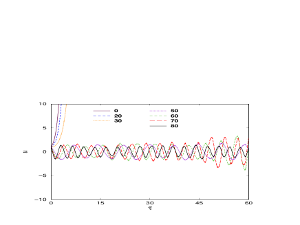
Figure 1: Solutions of (4) with $k=-1$ and $f(\tau)$ given by (10). When $A=0$, the solution increases exponentially, corresponding to the fact that the photon trajectories are unstable in a Universe with constant negative curvature. This is also the case when $A=20$ and $A=30$. When $A=50,60,70$ and 80 the solution is oscillatory, indicating stability.

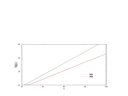
Figure 2: Plots of $\log u$ vs. $\tau$ for the data corresponding to A=20 and A=30 in Figure 1. The continuous black lines are best-fitting straight lines when $\tau>6$. For $A=20$ the gradient is about 0.85 (the theoretical value is $0.8498\ldots$). For $A=30$ the gradient is about 0.62 (the theoretical value is $0.6124\ldots$).

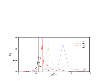
Figure 3: Plots of the fourier transform of the data for $u(\tau)$ shown in Figure 1, as a function of period $2\pi/\nu$ (i.e. $\nu$ is the frequency conjugate to $\tau$) when $A=50,60,70$ and 80. In each case the vertical dotted line marks the theoretical oscillation period, $2\pi/\sqrt{A^{2}/1440-1}$.

The above analysis generalizes directly to the geodesic deviation equation (3). This may be written as the stochastic matrix equation

$$\frac{d^{2}}{d\tau^{2}}\begin{pmatrix}\xi\\ \eta\end{pmatrix}=-\begin{pmatrix}K+Af_{11}(\tau)&Af_{12}(\tau)\\ Af_{12}(\tau)&K+Af_{22}(\tau)\end{pmatrix}\begin{pmatrix}\xi\\ \eta\end{pmatrix}.$$ (11)

The variables $\xi$ and $\eta$ can be separated into slow and fast components, as for $u$. Following the steps that led from (4) to (9) we find, in the high-frequency limit, that

$$\frac{d^{2}}{d\tau^{2}}\begin{pmatrix}\langle\xi\rangle\\ \langle\eta\rangle\end{pmatrix}\approx-(K\textbf{I}+A^{2}\langle\textbf{v}^{2}\rangle)\begin{pmatrix}\langle\xi\rangle\\ \langle\eta\rangle\end{pmatrix}$$ (12)

where I is the $2\times 2$ identity matrix and v is the matrix with elements $v_{ij}=\int^{\tau}f_{ij}(t)dt$, such that $\langle v_{ij}\rangle=0$. The stability of the trajectories thus depends on the eigenvalues of the matrix $K\textbf{I}+A^{2}\langle\textbf{v}^{2}\rangle$; specifically, assuming $\langle v_{11}\rangle=\langle v_{22}\rangle$, they are unstable if $A^{2}\langle(v_{11}\pm v_{12})^{2}\rangle<-K$, and if $A^{2}\langle(v_{11}\pm v_{12})^{2}\rangle>-K$ they are stable. Note that $v_{11}$ and $v_{12}$ are of the order of $\omega^{-1}$, and so the balance between the terms in the stability criterion depends on the size of $A^{2}/\omega^{2}|K|$. In particular, since $\omega$ is considered large here, if $K<0$ the perturbations must be large enough to cause the curvature to be positive in places for stabilization to occur. This is consistent with the fact that the geodesics on compact surfaces where the curvature is everywhere negative (but not necessarily constant) are strongly chaotic.

Let us make an order of magnitude estimate to determine the cosmological epoch when the stochastic term is observable. Since the curvature is small, it will always be dominated by an observable stochastic term (see below). Consider that the Universe consists of a volume fraction $(R_{*}/R)^{3}$ of clusters of galaxies of size $L\approx 1$Mpc and mass $M\approx 10^{-4}$Mpc in relativistic units. The number of clusters within a ball of radius $R$ is thus $\sim(R_{*}/L)^{3}$. The scale factor $R$ is set to the scale of the visible Universe at present, roughly $10^{4}$Mpc. $R_{*}$ is the distance scale at which voids between the galaxies began to form, at a redshift of order 10 (i.e. $R_{*}\sim 10^{3}$Mpc). The mean time (in terms of $\tau$) for a photon to move between clusters is of the order of $LR^{2}/R_{*}^{3}$. This gives $\omega\sim R_{*}^{3}/(LR^{2})$, which is large up to the present, but will fall to less than one in a few times the current age of the Universe, as the galaxies move apart. Note that $\omega$ is assumed large in the calculations described above.

The tidal forces $\Phi_{\xi\xi}$ are, up to factors of $4\pi$, of the order of the dimensionless density $MR^{2}/L^{3}$, from Poisson’s equation when a photon passes near a cluster; $Av$ is typically this quantity integrated over a mean free time, $MR^{4}/L^{2}R_{*}^{3}$. $|K|\lesssim 0.01$ in these units. The stochastic stabilization will be observable if $Av\gtrsim 1$, and will dominate the curvature if $Av/|K|\gtrsim 1$ (a weaker condition). Taking this together with the estimate for $\omega$, we conclude that stochastic stabilization is potentially observable when $(L^{2}/MR_{*})^{1/4}\lesssim R/R_{*}\lesssim(R_{*}/L)^{1/2}$; that is, for a period starting soon after the galaxies formed and due to end a few times the present age of the Universe from now. The magnitude of each deflection is determined by $M/L\sim 10^{-4}$, so this effect should be observable on angular scales of arcseconds or smaller [15]. From this perspective it should be easier to observe in distant quasars, which are almost pointlike, than the almost homogeneous cosmic background radiation.

The stochastic stabilization of photon trajectories has several interesting consequences for cosmology. In particular when $K\approx 0$ it is observable in the characteristic frequency with which neighbouring orbits oscillate about each other, corresponding to a periodic focusing and defocusing of distant images.

Given the recent focus on compact models of the Universe [11], we devote some concluding remarks to this case (although, as already noted, the mechanism is independent of topology). The simplest models of the Universe that go beyond having spatially constant negative curvature incorporate static fluctuations. Such models are to a large extent still unrealistic, because the curvature is unlikely to be static over the timescales associated with photon recurrence. Nevertheless, they illustrate most clearly the implications of stabilization, some of which we now list.

As a result of stabilization, the photon dynamics will generically possess both regular (stable) and irregular (chaotic) components, rather than being fully chaotic. While wave modes in fully chaotic systems are believed to have a gaussian value distribution, it is well established in the context of quantum chaos that regular trajectories lead to a quantifiable non-gaussian component whose precise form depends on the size and position of the regular regions in phase space [18]. This will in turn give rise to a non-gaussian component in the CMB, via the connection described in [8, 11]. There is, in addition, likely to be a second non-gaussian component due to the photon trajectories close to bifurcation (i.e. close to making the transition between instability and stability). It was established in [19] that bifurcations give rise to non-gaussian fluctuations in wave modes, quantified by characteristic scaling exponents in the wavelength dependence of the moments of their value distribution in the short-wavelength limit. In situations when all of the generic bifurcations contribute, the moment exponents take on universal values, which were calculated in [19]. These non-gaussian statistics are also likely to feed through to the fluctuations in the CMB in the models under consideration here.

Bifurcations have a strong influence on the scarring of wave modes as well. In fully chaotic systems wave modes may be scarred by periodic orbits [13]. This effect is dramatically enhanced when the orbits undergo bifurcation [19], giving rise to superscars. It has been suggested by Levin and Barrow, in the context of constant negative curvature models, that scars may give rise to anisotropic structures in the CMB [8, 11]. This mechanism would therefore be strongly enhanced by stabilization. Levin and Barrow [8, 11] have also put forward the idea that the anisotropic structures associated with scars may show up in the distribution of matter. Regions of regular motion and superscars would significantly amplify this effect. In particular, stable islands typically have a fractal distribution, and this may provide an explanation, within the context of their theory, for the fractal hierarchy of structures seen in galaxies and clusters of galaxies. Stable orbits also strongly inhibit the rate of mixing, giving rise to intermittency, and so may play a role in the suggested links between mixing and preinflationary homogenization [7].

We gratefully acknowledge very helpful discussions with Dr Gopal Basak and Professors Sir Michael Berry and Mark Birkinshaw.

References

- [1]
- [2] P. J. E. Peebles, in The Large-scale Structure of the Universe (Princeton Univ. Press, Princeton, 1980).
- [3] P. L. Kapitsa, Zh. Eksperim. Teor. Fiz. 21, 588 (1951).
- [4] C. L. Bennett et al., Astrophys. J. Suppl. S. 148, 1 (2003).
- [5] V. G. Gurzadyan and A. A. Kocharyan, Astron. Astrophys. 260, 14 (1992).
- [6] M. Lachièze-Rey and J. P. Luminet, Phys. Rep. 254, 135 (1995).
- [7] N. J. Cornish, D. N. Spergel and G. D. Starkman Phys. Rev. Lett. 77, 215 (1996).
- [8] J. Levin and J. D. Barrow, Class. Quantum Grav. 17, L61 (2000).
- [9] J. D. Barrow and J. Levin, Phys. Rev. A 63, 044104 (2001).
- [10] R. Aurich and F. Steiner, Mon. Not. R. Astron. Soc. 323, 1016 (2001).
- [11] J. Levin, Phys. Rep. 365, 251 (2002).
- [12] M. V. Berry, J. Phys. A 10, 2083 (1977).
- [13] E. J. Heller, Phys. Rev. Lett. 53, 1515 (1984).
- [14] V. F. Mukhanov, H. A. Feldman and R. H. Brandenberger, Phys. Rep. 215, 203 (1992).
- [15] U. Seljak, Astrophys. J.463, 1 (1996).
- [16] C. W. Misner, K. S. Thorne and J. A. Wheeler, Gravitation (Freeman, 1973).
- [17] J. Kao and V. Wihstutz, Stochastics and Stochastic Reports 49, 1 (1994).
- [18] A. Bäcker and R. Schubert, J. Phys. A 35, 527 (2002).
- [19] J. P. Keating and S. D. Prado, Proc. R. Soc. London, Ser. A 457, 1855 (2001).