Response maxima in modulated turbulence

Abstract

Isotropic and homogeneous turbulence driven by an energy input modulated in time is studied within a variable range mean-field theory. The response of the system, observed in the second order moment of the large-scale velocity difference $D(L,t)=\langle\!\langle({\mbox{\boldmath$u$}}(x+L)-{\mbox{\boldmath$u$}}(x))^{2}\rangle\!\rangle\propto Re^{2}(t)$, is calculated for varying modulation frequencies $\omega$ and weak modulation amplitudes. For low frequencies the system follows the modulation of the driving with almost constant amplitude, whereas for higher driving frequencies the amplitude of the response decreases on average $\propto 1/\omega$. In addition, at certain frequencies the amplitude of the response either almost vanishes or is strongly enhanced. These frequencies are connected with the frequency scale of the energy cascade and multiples thereof.

I Introduction

Many turbulent flows are characterized by time dependent forcing. E.g. the atmosphere of the earth is driven by the heating through the radiation from the sun, the blood flow in the arteries by the heart beats, etc. Also technical flows like the flow in the intake of a combustion engine are periodically forced. Another example are estuaries and adjacent coastal waters, where tidal straining leads to a periodic alternation of stratification and turbulent mixing of saline and fresh water Rippeth et al. (2001). This results in a periodically varying energy dissipation in the upper water layers with a 12 hour period.

The effect of a periodically increasing and decreasing energy input on turbulent flow depends on the frequency of the driving. This has been studied in reference Scotti and Piomelli (2001) for a turbulent channel flow where the modulations of the input rate are generated near the wall. It was found that for high frequencies these oscillations are strongly damped with distance from the walls, such that they do not reach the inner part of the logarithmic boundary layer. Another example is Rayleigh-Benard convection: the interaction between the large scale circulating flow and the thermal plumes detaching from the upper and the lower boundary layers acts as a stochastically influenced time-dependent forcing on the turbulent flow in the inner region of the cell, as recently shown in Qiu et al. (2000); Qiu and Tong (2001a, b). In a von Kármán flow between two coaxial corotating disks Labbé et al. (1996); Aumaître et al. (2000), the energy input rate is not constant if the disks are kept rotating at constant speed, but is periodically varying with a geometry-dependent frequency due to a coherent vortex precessing around the axis of rotation. In this case it was also shown, that the statistical properties of the turbulent fluctuations are affected by the time dependence of the mean flow. However, the averaged velocity power spectrum still shows Kolmogorov scaling over a broad frequency range, in addition to a low frequency peak corresponding to the oscillation of the mean flow.

These results raise the question how global quantities of a turbulent flow, like e.g. the total energy or the Reynolds number, respond to a time dependent energy input. This problem is the subject of the present paper. From a more fundamental point of view, studying modulated turbulence will give more insight into the time scales in particular of the turbulent energy cascade.

In a previous study Lohse (2000), the time evolution of the Reynolds number in a periodically kicked flow was analyzed. If the kicking strength and the kicking frequency are large enough, the Reynolds number grows and saturates on a level, which depends on the frequency and the kicking strength. The theoretical results from Lohse (2000) have later been verified numerically in reference Hooghoudt et al. (2001).

In this present paper, we study a related type of forcing. Rather than periodically kicking the boundary conditions of homogeneous, isotropic turbulence as in Lohse (2000), we force the flow through a time-dependent modulation of the energy input rate $e_{in}(t)$ on the outer length scale $L$,

$$e_{in}(t)=e_{0}(1+e\sin(\omega t)).$$ (1)

This means that the flow is stationarily stirred ($\propto e_{0}$) to maintain the turbulent flow and, in addition, a time-dependent modulation of the forcing ($\propto e_{0}e$) is applied, $0\leq e\leq 1$. The response of the system to the time-dependent stirring can be observed e.g. in the second order velocity structure function of the flow field, in particular at the outer scale $L$, $D(L,t)=\langle\!\langle({\mbox{\boldmath$u$}}({\mbox{\boldmath$x$}}+{\mbox{\boldmath$L$}},t)-{\mbox{\boldmath$u$}}({\mbox{\boldmath$x$}},t))^{2}\rangle\!\rangle$. This $D(L,t)$ is equivalent to a Reynolds number, which we define as $Re=u_{1,rms}L/\nu$. Here, $u_{1,rms}(t)$ is the rms of one component of the velocity, varying with time $t$. Then, disregarding correlations on scale $L$,

$$D(L,t)=2\langle\!\langle{\mbox{\boldmath$u$}}^{2}\rangle\!\rangle=6u_{1,rms}^{2}(t)=\frac{6\nu^{2}Re(t)^{2}}{L^{2}}.$$ (2)

The energy put into the system at time $t$ will travel down the energy cascade towards smaller scales and will, on average, be dissipated at time $t+\tau$, i.e., with a mean time delay $\tau$. In other words, the dissipation at time $t$ depends on how much energy has been in the large scales at time $t-\tau$. We approximately describe the relevant time scale $\tau$ for the cascade process by the large eddy turnover time $\tau_{L}$ at that time $t-\tau$,

$$\tau\simeq\tau_{L}={L\over u_{1,rms}(t-\tau)}={L\over\sqrt{D(L,t-\tau)/6}}.$$ (3)

More accurately, the time scale of the energy cascade is given by the sum over the eddy turnover times on all decay steps, $\tau\simeq\sum_{n}\tau_{n}$. In this sum, the largest contribution is the largest eddy turnover time $\tau_{L}$. For K41 scaling the smaller eddies $r_{n}/L=\delta^{n}$, where $0<\delta<1$, have turnover times $\tau_{n}=\tau_{L}\delta^{2n/3}$. Thus $\tau=\tau_{L}\sum_{n}\delta^{2n/3}\equiv\tau_{L}a$. The common choice $\delta=1/2$ implies $a\simeq 2.7$. Putting into intermittency corrections gives slightly smaller values of $a$. In this present paper we shall discuss the influence of $a$ by comparing the limiting cases $a=2.7$ and $a=1$. Experimentally, in principle the parameter $a$ could be measured by analyzing the positions, heights and widths of the response maxima, thus giving information about the energy cascade time.

If the external modulation period $\omega^{-1}$ is much larger than this intrinsic time scale $\tau$, $\omega\tau\ll 1$, the turbulent flow will have time to adjust and will follow the periodic variations of the stirring. If, on the other hand, $\omega^{-1}$ is decreased and becomes much smaller than $\tau$, the system can follow less and less, and feels, at small scales, an average time-independent energy input.

We calculate the time dependence of the response $D(L,t)-D_{0}(L)$ to a periodically modulated energy input rate, Eq. (1), within a variable scale mean-field theory Effinger and Grossmann (1987) for various driving frequencies $\omega$. Here, $D_{0}(L)$ is the second order structure function for a stationary energy input rate $e_{0}$. In general, the energy flow rate through the system is an intermittently fluctuating quantity. Therefore, the cascade time as well as the response of the system are fluctuating. These fluctuations are neglected by the mean-field theory in the present study. However, on average these fluctuations result in a mean downscale transport of energy which controls the overall properties of the flow. Therefore, we believe that within this mean-field approach we can grasp the main features of the flow correctly.

The method is explained in the next section. The behavior of the response as a function of the driving frequency $\omega$ in the case of weak modulations of the energy input rate is analyzed in section III. In section IV we discuss an alternative way to introduce time dependence into the system. The slightly different case of a modulated driving force instead of a modulated energy input rate is presented in section V. We summarize our results in section VI.

II Method and Model

In reference Effinger and Grossmann (1987) an energy balance equation for the second order velocity structure function $D(r)=\langle\!\langle({\mbox{\boldmath$u$}}({\mbox{\boldmath$x$}}+{\mbox{\boldmath$r$}})-{\mbox{\boldmath$u$}}({\mbox{\boldmath$x$}}))^{2}\rangle\!\rangle$ for stationary, homogeneous, and isotropic turbulence has been derived within a variable range mean-field theory. Here, $u$ is the velocity and the brackets $\langle\!\langle...\rangle\!\rangle$ denote the ensemble average. One of the essentials of this theory is to divide the velocity field into a (spatially averaged) superscale velocity ${\mbox{\boldmath$u$}}^{(r)}$ and a (strongly fluctuating) subscale velocity $\tilde{\mbox{\boldmath$u$}}^{(r)}$. The spatial average is performed over a sphere of variable radius $r$, and will be denoted as ${\mbox{\boldmath$u$}}^{(r)}({\mbox{\boldmath$x$}})\equiv\langle{\mbox{\boldmath$u$}}({\mbox{\boldmath$x$}}+{\mbox{\boldmath$y$}})\rangle^{(r)}_{y}\equiv{3\over 4\pi r^{3}}\int_{|{\mbox{\boldmath$y$}}|\leq r}d^{3}y\ {\mbox{\boldmath$u$}}({\mbox{\boldmath$x$}}+{\mbox{\boldmath$y$}})$.

The energy input rate $e_{in}$, which in the statistically stationary situation equals the total energy dissipation rate $\epsilon$, is balanced in accordance with the super- and subscale decomposition by the energy dissipation rate on all scales larger than $r$ complemented by the energy transfer across scale $r$ from the super- to the subscales of $r$. In a simplified version the derived energy balance equation reads:

$$e_{in}=\epsilon={3\over 2}\left(\nu+\frac{D(r)^{2}}{b^{3}\epsilon}\right){1\over r}{d\over dr}D(r),$$ (4)

where $\nu$ is the kinematic viscosity and $b$ the Kolmogorov constant. In the viscous subrange (VSR), where $r$ is smaller than the Kolmogorov length scale $\eta$, $r<\eta$, the dissipation term, i.e., the first term on the rhs of Eq. (4), is dominating, and therefore the solution of Eq. (4) is $D(r)=\epsilon r^{2}/3\nu$. In the inertial subrange, instead, where $\eta\ll r\ll L$, most of the energy of the eddies is transfered down-scale. This energy transfer rate $E_{t}$, which is given by the second term on the rhs of Eq. (4), is determined by the decorrelation rate $\tilde{\Gamma}(r)$ of the subscale eddies, which itself is mainly governed by the energy dissipation rate $\epsilon$, see Effinger and Grossmann (1987) for details. Note again that in the stationary case the energy dissipation rate equals the energy input rate, $\epsilon=e_{in}$. In the ISR the second term on the rhs is the leading one. Then the solution of Eq. (4) is $D(r)=b(\epsilon r)^{2/3}$. The full energy rate balance equation (4) interpolates between these two limits. The Kolmogorov constant $b$ can be calculated within this theory to be $b=6.3$ which is consistent with the experimental value Monin and Yaglom (1975); Sreenivasan (1995); Sreenivasan and Antonia (1997); Pope (2000).

In our case the flow is not stationary but experiences a modulated energy input rate $e_{in}(t)$. Therefore, $e_{in}$, the structure function $D(r)$, and the dissipation rate $\epsilon$ in Eq. (4) will depend on time. Furthermore, an additional term on the rhs of Eq. (4) appears, taking into account the non-stationarity of the flow:

$$e_{in}(t) = {3\over 2}\left(\nu+\frac{D(r,t)^{2}}{b^{3}\epsilon(t)}\right){1\over r}{\partial\over\partial r}D(r,t)$$

$$+{1\over 2}{\partial\over\partial t}\langle\!\langle{\mbox{\boldmath$u$}}^{(r)}({\mbox{\boldmath$x$}},t)\cdot{\mbox{\boldmath$u$}}^{(r)}({\mbox{\boldmath$x$}},t)\rangle\!\rangle.$$

The correlation of the superscale velocities can be written as $\langle\!\langle{\mbox{\boldmath$u$}}^{(r)}({\mbox{\boldmath$x$}},t)\cdot{\mbox{\boldmath$u$}}^{(r)}({\mbox{\boldmath$x$}},t)\rangle\!\rangle=\langle\!\langle{\mbox{\boldmath$u$}}^{2}({\mbox{\boldmath$x$}},t)\rangle\!\rangle-{1\over 2}\langle\langle D(y_{1}+y_{2},t)\rangle^{(r)}_{y_{1}}\rangle^{(r)}_{y_{2}}$. Following the arguments in Effinger and Grossmann (1987) for the derivation of Eq. (4), we neglect multiple spatial averaging, i.e., $\langle\langle D(y_{1}+y_{2},t)\rangle^{(r)}_{y_{1}}\rangle^{(r)}_{y_{2}}\simeq\langle D(y,t)\rangle^{(r)}_{y}$.

In the stationary case the energy dissipation rate $\epsilon=\nu\langle\!\langle\frac{\partial u_{i}}{\partial x_{j}}\frac{\partial u_{i}}{\partial x_{j}}\rangle\!\rangle$ can be related to the large scale quantities by

$$\epsilon=c_{\epsilon}\frac{u_{1,rms}^{3}}{L}=c_{\epsilon}(D(L))\frac{D(L)^{3/2}}{6^{3/2}L}.$$ (6)

Extending this expression to the time-dependent case, we have to take into account that the energy which is fed into the system on large scales at a time $t$ will be dissipated on small scales at a later time $t+\tau$. We model this as follows: The energy dissipation rate at time $t$ is assumed to depend on the large scale quantities at time $t-\tau$:

$$\epsilon(t)=c_{\epsilon}(D(L,t-\tau))\frac{D(L,t-\tau)^{3/2}}{6^{3/2}L}.$$ (7)

$c_{\epsilon}$ is a dimensionless function which is approximately constant ($\simeq 1$) for very large Reynolds numbers Sreenivasan (1984, 1998). In Lohse (1994); Grossmann (1995); Stolovitzky and Sreenivasan (1995) it was shown that in general $c_{\epsilon}$ depends on the Reynolds number, and therefore on $D(L)$. We here use an approximation of the expression derived in Lohse (1994) for high Reynolds numbers:

$$c_{\epsilon}(D(L)) = {9\over Re}+\sqrt{\left({6\over b}\right)^{3}+\left({9\over Re}\right)^{2}}$$

$$\simeq \left({6\over b}\right)^{3/2}+\frac{9}{Re}=\left({6\over b}\right)^{3/2}+9{\nu\over L}\sqrt{6\over{D(L)}}.$$

The delay time $\tau$ is determined by the implicit time-delay equation (3). Assuming that the solution of Eq. (4) in the ISR, $D(r)=b(\epsilon r)^{2/3}$, is valid up to $r=L$, we can write $D(r)=\left(\frac{r}{L}\right)^{2/3}D(L)$. Within our model, where we connect small and large scale quantities at different times, the structure function on scale $r<L$ at time $t$ will depend on the large scale structure function at an earlier time $t-\tau$, i.e., we introduce $D(r,t)=\left({r\over L}\right)^{2/3}D(L,t-\tau)$ into Eq. (II). After multiplying with $r$, Eq. (II) can be integrated from $r=0$ up to the outer length scale $r=L$:

$${1\over 4}{d\over dt}(D(L,t)-\alpha D(L,t-\tau)) = -\frac{D(L,t-\tau)^{3/2}}{Lb^{3/2}}$$ (9)

$$-\frac{3\nu D(L,t-\tau)}{2L^{2}}$$

$$+e_{in}(t),$$

where $\alpha={27\over 44}$ originates from the integration. In Effinger and Grossmann (1987) it has been shown that, in the isotropic and homogenous case, $e_{in}$ is independent of the scale $r$ as the forcing is assumed to act on the largest scale $L$ only. In the stationary case the lhs of Eq. (9) vanishes, and together with Eqs. (7) and (II), Eq. (9) corresponds to $\epsilon=e_{in}$. Eq. (9) contains only large scale quantities. Effects of fluctuations in the energy input rate on the statistical properties of the turbulent flow as observed in Labbé et al. (1996) would influence the scaling behavior of $D(r,t)$ on intermediate scales $r$ and therefore lead to different values of the factor $\alpha$, but the structure of Eq. (9) would remain the same.

Using Eq. (2), we express the second order structure function $D(L,t)$ in Eq. (9) in terms of the Reynolds number $Re(t)$:

$${L^{2}\over\nu}\!{d\over dt}(Re^{2}(t)\!-\!\alpha Re^{2}(t\!-\!\tau))\! \!=\! \!-{2\over 3}\!\left({6\over b}\right)^{3/2}\!(Re^{2}(t\!-\!\tau))^{3/2}$$

$$-6Re^{2}(t-\tau)$$

$$+{2\over 3}\frac{e_{0}L^{4}}{\nu^{3}}(1+e\sin{\omega t}).$$

Here, we have inserted the time-dependent energy input rate, Eq. (1). In the case a of constant energy input rate, i.e., $e=0$, Eq. (II) simplifies to

$$0=-\frac{2}{3}\left({6\over b}\right)^{3/2}Re_{0}^{3}-6Re_{0}^{2}+\frac{2}{3}\frac{L^{4}}{\nu^{3}}e_{0},$$ (11)

relating the stationary Reynolds number $Re_{0}$ to the stationary input rate, $\frac{L^{4}}{\nu^{3}}e_{0}(Re_{0})=c_{\epsilon}(Re_{0})Re_{0}^{3}$. Introducing the reduced Reynolds number $R(t)\equiv Re(t)/Re_{0}$ and the non-dimensional time $t/\tau_{L}^{0}$ as $t$ (analogously for $\tau$ and $\omega$), Eq. (II) becomes

$$\frac{d(R^{2}(t)\!-\!\alpha R^{2}(t\!-\!\tau))}{dt}\! \!=\! \!-{2\over 3}\left({6\over b}\right)^{3/2}(R^{2}(t\!-\!\tau))^{3/2}$$

$$- \frac{6}{Re_{0}}R^{2}(t-\tau)$$

$$+ \!\left(\!{2\over 3}\!(6/b)^{3/2}+\!\frac{6}{Re_{0}}\!\right)\!(\!1\!+\!e\sin{\omega t}\!).$$

Here, $\tau_{L}^{0}=\frac{L}{u^{0}_{1,rms}}$ is the large eddy turnover time of the stationary flow. $R(t)$ is of order one. The delay time $\tau$ in units of the time scale $\tau_{L}^{0}$ is given by

$$\tau=\frac{a}{R(t-\tau)}.$$ (13)

Eq. (II) describes the time evolution of $R^{2}(t)$, which is the square of the Reynolds number of a flow exposed to a modulated energy input rate (Eq. (1)), normalized by the square of the Reynolds number of a flow where only a constant, time-independent, forcing is applied.

III Response of turbulent flow to energy input rate modulations

III.1 General trend

In the present study we shall restrict ourselves to the case of weak amplitude modulation, i.e., $e$ in Eq. (1) is small. Then we expect that also the oscillating response

$$\Delta(t)\equiv R^{2}(t)-1$$ (14)

has a small amplitude, and we can linearize Eq. (II). The time delay $\tau$ is approximated by a time-independent constant which in our time units $\tau_{L}^{0}$ is simply $a$. This approximation is justified as long as $|\Delta|\ll 1$. In section III.3 we shall discuss the limits of this approximation. We first consider $a=1$ which means that the cascade time $\tau$ is taken as the large eddy turnover time $\tau_{L}^{0}$. The resulting equation of motion for the response $\Delta(t)$,

$${d\over dt}(\Delta(t)-\alpha\Delta(t-\tau)) = -\left(\left(\frac{6}{b}\right)^{3/2}+\frac{6}{Re_{0}}\right)\Delta(t-\tau)$$

$$+\left({2\over 3}(\left(\frac{6}{b}\right)^{3/2}+\frac{6}{Re_{0}}\right)e\sin{\omega t},$$

can be solved analytically. The solution to the linear equation (LABEL:lineq) can be calculated using the ansatz:

$$\Delta(t)=eA(\omega)\sin{(\omega t+\phi)}.$$ (16)

Here, $A(\omega)$ is the amplitude, and $\phi$ is the phase shift of the response which also depends on $\omega$. Inserting this expression into Eq. (LABEL:lineq) gives the explicit solution of the linear response equation (LABEL:lineq):

$$\Delta(t)=e\frac{\left({2\over 3}\left(\frac{6}{b}\right)^{3/2}+\frac{6}{Re_{0}}\right)}{\omega}\frac{\Big{[}-\cos{\omega t}+\alpha\cos{\Big{(}\omega(t+\tau)\Big{)}}+\frac{\left(\frac{6}{b}\right)^{3/2}+{6\over Re_{0}}}{\omega}\sin{\Big{(}\omega(t+\tau)\Big{)}}\Big{]}}{(1+\alpha^{2}+\left(\frac{\left(\frac{6}{b}\right)^{3/2}+\frac{6}{Re_{0}}}{\omega}\right)^{2}-2\alpha\cos{\omega\tau}-2\frac{\left(\frac{6}{b}\right)^{3/2}+\frac{6}{Re_{0}}}{\omega}\sin{\omega\tau})}.$$ (17)

In the following, we set the Kolmogorov constant $b=6$ for simplicity, which is near to the calculated value 6.3 Effinger and Grossmann (1987) and to the experimental value in the range $6-9$ Monin and Yaglom (1975); Sreenivasan (1995); Sreenivasan and Antonia (1997); Pope (2000). To recover the expressions for a general $b$ one has to replace in the following results the terms $(1+{6\over Re_{0}})$ and $({2\over 3}+{6\over Re_{0}})$ by $((6/b)^{3/2}+{6\over Re_{0}})$ and $({2\over 3}(6/b)^{3/2}+{6\over Re_{0}})$, respectively. The mean amplitude of the response is determined by the energy input rate $({2\over 3}+{6\over Re_{0}})e$, i.e., the last term on the rhs of Eq. (LABEL:lineq). The time derivative on the lhs of Eq. (LABEL:lineq) leads to a mean decrease of the amplitude as $1/\omega$. Due to the two terms in Eq. (LABEL:lineq) containing the time delay $\tau=a$, corresponding terms in the second fraction of the solution (17) appear, $\propto\alpha$ and $\propto(1+{6\over Re_{0}})/\omega$, respectively, which, by the periodic dependence on $\omega\tau$ induce a periodic variation of the amplitude with the frequency $\omega$. For low frequencies the terms $\propto(1+6/Re_{0})/\omega$, originating from the first term on the rhs of Eq. (LABEL:lineq), dominate, whereas for high frequencies the terms $\propto\alpha$, due to the second term on the lhs of Eq. (LABEL:lineq), become more important. The latter, in particular, lead to a periodic variation of the response amplitude up to very high frequencies.

The linear response $\Delta(t)\propto e$ of the flow (with $Re_{0}=10^{4}$) is plotted in Fig.1 for four different modulation frequencies. Also the modulation of the energy input rate, $e_{in}(t)/e_{0}-1$ is plotted in Fig.1.

Figure 1: Response $\Delta(t)$ (solid lines) for four different modulation frequencies $\omega$, the time dependent part of the energy input rate, $e_{in}(t)/e_{0}-1$ (dotted lines). The modulation amplitude is $10\%$ of the constant input rate, $e=0.1$, and the Reynolds number of the stationary system is chosen as $Re_{0}=10^{4}$. (a) $\omega\tau_{L}^{0}=10^{-3}$, (b) $\omega\tau_{L}^{0}=0.1$, (c) $\omega\tau_{L}^{0}=10$, (d) $\omega\tau_{L}^{0}=100$.

The deviation of the Reynolds number from its stationary value $Re_{0}$, $\Delta(t)=(Re^{2}(t)-Re_{0}^{2})/Re_{0}^{2}$, oscillates with the same frequency as the driving, for all frequencies $\omega$. The amplitude $A$ of this oscillation depends on the frequency. For the two small modulation frequencies, $\omega=10^{-3}$ and $\omega=10^{-1}$, the amplitude of the response $\Delta(t)$ is nearly the same, about two thirds of the amplitude $e$ of the driving. For higher frequencies, the amplitude $A$ of the response decreases. In the case of $\omega=10$ we observe a phase shift between the forcing and the resulting response.

Figure 2: (a) Amplitude $A$ of the response $\Delta(t)$ as a function of the driving frequency $\omega$ (log-log-scale) for weak modulations ($e=0.1$) of the input rate $e_{in}$, and $Re_{0}=10^{4}$. The time scale of the energy cascade is set to $\tau=a=1$. The dashed line denotes the low frequency limit of the oscillation amplitude, $2/3$, and the dotted line corresponds to the mean trend of the high frequency limit, $\frac{2}{3}\frac{1}{\omega\tau_{L}^{0}}$. Inset: linear-scale-plot of the response amplitude versus frequency. The small arrows indicate the frequencies $\omega_{r}$ (in units of $\tau_{L}^{0}$) of the response extrema calculated from the extrema of the denominator in Eq. (17). The horizontal arrow denotes the frequency distance $\Delta\omega$ (in units of $\tau_{L}^{0}$) between two frequencies for which the amplitude is maximal (or minimal). It is $\Delta\omega\simeq 2\pi/\tau$ for high frequencies. (b) Same as (a) but with a cascade time scale $\tau=a=2.7$ different from the large eddy turnover time $\tau_{L}^{0}$. Note the shift of the response maxima, the less pronounced height and greater width of the first, and the more pronounced second response peak.

Fig.2a shows the amplitude $A(\omega)$ as a function of the driving frequency for $Re_{0}=10^{4}$. For low frequencies the amplitude remains constant, and is two thirds, whereas for large frequencies the amplitude of the response $\Delta(t)$ decreases $\propto 1/\omega$. In addition to this decrease we note certain frequencies for which the response amplitude becomes large or very small. The distance between two maxima or two minima of the amplitude is nearly constant, see the inset of Fig.2a. This periodic behavior in the $\omega$-dependence of the response amplitude is due to the time delay $\tau$. We shall explain this in the next section.

There are three time scales in the solution (17) of Eq. (LABEL:lineq): The large eddy turnover time, by definition 1, the time delay $\tau=a$, which represents the cascade time, and the time scale of the external modulation $1/\omega$. If the modulation time scale is much larger than the large eddy turnover time, $1/\omega\gg 1$, i.e., if the driving frequency is very small, then the solution (17) can be approximated by

$$\Delta(t)\simeq e{2\over 3}\sin{\Big{(}\omega(t+\tau)\Big{)}}.$$ (18)

We conclude $A=2/3$, while the phase $\phi=\omega\tau$ is linear in $\omega$ for small frequencies.

If, on the other hand, the modulation frequency becomes very large, i.e, the time scale of the driving is much smaller than $1$, we see from Eq. (17) that the amplitude of $\Delta$ decreases as $\propto 1/\omega$:

$$\Delta(t)\simeq e\frac{({2\over 3}+{6\over Re_{0}})}{\omega}\frac{\Big{[}-\cos{\omega t}+\alpha\cos{\Big{(}\omega(t+\tau)\Big{)}}\Big{]}}{1+\alpha^{2}-2\alpha\cos{\omega\tau}}.$$ (19)

The mean trend $\propto\frac{({2\over 3}+{6\over Re_{0}})}{\omega}\simeq\frac{2}{3\omega}$ of this high frequency limit is also plotted in Fig.2a. The crossover between the regimes of Eq. (18) and (19) takes place at $\omega_{cross}\simeq 1$. This can be seen in Fig.2a. The crossover frequency is not changed by taking into account the cascade time $\tau=a\not=1$, as can be seen in Fig.2b which shows the response amplitude as a function of frequency for $a=2.7$.

We have considered here only the case, where the Kolmogorov constant $b=6$. For a general $b$, the crossover frequency is at $\omega_{cross}\simeq\left(6/b\right)^{3/2}$, as can be seen from the solution (17). This means, that the crossover from the regime of constant amplitude to the regime of $1/\omega$-decay takes place at a smaller frequency if $b$ is larger. The positions of the response maxima, however, are only slightly shifted by a different $b$.

In conclusion, as long as the modulation frequency of the energy input rate is smaller than $1$, i.e., the large eddy turnover time is shorter than the period of the forcing, the system has time to follow the periodic modulations with an almost constant amplitude. For higher frequencies instead, the oscillations become too fast for the system to follow, and therefore, the response becomes weaker and weaker, and phase shifted. Then the system experiences the fast modulation more and more as a constant average energy input, and the oscillations of the response vanish as $1/\omega$. This high frequency behavior has also been found for spin systems driven by an oscillating magnetic field Rao et al. (1990).

III.2 Response maxima

In Fig.2 we have seen that there are certain frequencies for which the amplitude of the response becomes large or very small. Mathematically, these response extrema originate from the minima and maxima of the denominator in Eq. (17),

$$N(\omega)= \omega \Big{[}1+\alpha^{2}+\left(\frac{1+{6\over Re_{0}}}{\omega}\right)^{2}$$

$$-2\alpha\cos{\omega\tau}-2\frac{1+{6\over Re_{0}}}{\omega}\sin{\omega\tau}\Big{]}.$$

We calculate the extrema of $N(\omega)$ numerically. The first few of them are indicated by the small arrows in Fig.2a. The lowest frequency is near to $\omega_{r1}\simeq\pi/3\tau\simeq 1$. There, the first and strongest maximum of the response can be observed, where the amplitude becomes as high as $A\simeq 4.2$. Note, that this frequency is nearly equal to the crossover frequency $\omega_{cross}$ between the low and high frequency regimes of Eq. (18) and (19) only in this particular case, where $a=1$. If we assume an energy cascade time $\tau=a=2.7$ the frequencies of the maxima are shifted towards smaller frequencies. The height of the first maximum is decreased, i.e., $A\simeq 1.2$, whereas the height of the following maxima is slightly increased, see Fig.2b. For very large frequencies, $\omega\gg 1$, we can estimate the frequencies of the response extrema also analytically. Then the two terms in the denominator $\propto\frac{1+{6\over Re_{0}}}{\omega}$ can be neglected, and the extrema of $N(\omega)$ can be approximated by the extrema of $\cos{\omega\tau}$,

$$\omega_{r}(n)\simeq n{\pi\over\tau},\qquad n=0,\pm 1,\pm 2,...\ .$$ (21)

Now the amplitude of $\Delta$ is at maximum for frequencies $\omega_{r}(n)$ with even $n$, and at minimum for $\omega_{r}(n)$ with odd $n$. The distance between two maximum (or minimum) amplitudes is $2\pi/\tau$ as indicated by the horizontal arrow in the inset of Fig.2. For the first maxima and minima at moderate frequencies this estimate is an approximation only; also their distances are not yet constant as they are for high frequencies.

In the high frequency limit, the oscillation of the response at the frequencies $\omega_{r}$ of maximum or minimum amplitude is phase shifted by $\phi_{r}(m)=(2m+1)\pi/2$, $m=\pm 1,\pm 3,...$:

$$\Delta(t)=e\frac{({2\over 3}+{6\over Re_{0}})}{\omega_{r}}\frac{(-1\pm\alpha)\cos{\omega_{r}t}}{(1\mp\alpha)^{2}}\propto\sin{(\omega_{r}t+\phi_{r})}.$$ (22)

The prefactor $(-1\pm\alpha)$ is always negative, i.e., at the response extrema we have $\Delta(t)\propto-\cos\omega_{r}t=\sin(\omega_{r}t+\phi_{r})$. In Fig.3 the phase shift $\phi(\omega)$, calculated from the solution (17), is shown as a function of the driving frequency $\omega$ for all frequencies. As the phase shift starts with $\phi(\omega=0)=0$ and changes continuously with increasing frequency, we find that only $m=1$ is possible for the phase shift $\phi_{r}$ at the response extrema. The frequencies of the maximum and minimum amplitudes of $\Delta$ are indicated by arrows. The only exception is the first maximum, where the approximation for $\omega_{r}$, Eq. (21) does not yet hold. There, the phase shift is near to $\pi/2$, corresponding to $m=0$.

Figure 3: (a) Phase shift $\phi(\omega)$ as a function of the modulation frequency $\omega$ for weak modulation strength $e=0.1$, and $Re_{0}=10^{4}$. The upper (lower) arrows indicate the frequencies of maximum (minimum) amplitude of the response. For small $\omega$ the phase $\phi(\omega)\propto\omega\tau$ behaves linearly.

Another phase shift in this model is the one between the response $\Delta(t)$ and the energy dissipation rate $\epsilon(t)$. According to Eq. (7) the dissipation rate is phase shifted by $-\omega\tau$ with respect to the response $\Delta(t)$, i.e., this shift is linearly growing with increasing frequency $\omega$. At the response maxima and minima the phase shift is $-\omega_{r}\tau\simeq-n\pi$.

The physics behind these response extrema can be explained as follows: The time delay $\tau$ can be regarded as the (average) time which the input energy needs before it is dissipated at small scales. In the case of maximum amplitude of the response the time delay $\tau$ is a multiple $jT$ of the period $T=2\pi/\omega$ of the forcing, whereas for the frequencies of minimum amplitude the delay $\tau$ has an additional $T/2$. Therefore, at the extrema of the response, the energy dissipation rate and the response are either in phase (maxima) or anti-phased (minima). In the latter case the oscillation of the response is strongly reduced. If, on the other hand, the driving frequency is such that the response and the dissipation rate are in phase, the transport of energy through the system is very effective and leads to an enhanced oscillation. At the response maxima as well as at the minima the phase shift between energy input rate and response is $\phi_{r}=3\pi/2$.

III.3 Quality of the approximation for the delay $\tau$

In the above calculations we made an approximation for the time scale $\tau$ of the cascade process. In the linearized model, we assumed $\tau$ to be constant, $\tau=\tau_{0}=a$. Now we check a posteriori the quality of this approximation. The solution (17) of the linearized equation (LABEL:lineq) is used to compute the “correct” delay time $\tau$ step by step: The next approximation for $\tau$ is

$$\tau_{1}(t)=\frac{a}{\sqrt{1+\Delta(t)}},$$ (23)

where the delay in Eq. (13) is still neglected. Further steps are:

$$\tau_{2}(t) = \frac{a}{\sqrt{1+\Delta(t-\tau_{1})}},$$ (24)

$$\tau_{3}(t) = \frac{a}{\sqrt{1+\Delta(t-\tau_{2})}},\quad\mbox{etc.}$$

In Fig.4 $\tau_{0}=a$, $\tau_{1}$, $\tau_{2}$, and $\tau_{3}$ are plotted for different frequencies. For $\omega=0.01$, the difference between $\tau_{1}$, $\tau_{2}$, and $\tau_{3}$ is not visible. The variation of the $\tau_{i}(t)$, ($i=1,2,3$), is largest at the frequency where the amplitude of $\Delta$ is maximum, i.e., at $\omega\simeq{1\over\tau_{0}}$. For all other frequencies, including at the response maxima, the variation of the $\tau_{i}(t)$ is much smaller than $\tau_{0}$ and $1/\omega$. At these frequencies it seems reasonable to approximate $\tau$ by the constant $\tau_{0}=a$. In Eq. (LABEL:lineq) the delay $\tau$ enters into two terms, in $\propto\partial_{t}\Delta(t-\tau)$ on the lhs, and in $\propto\Delta(t-\tau)$ on the rhs. We calculate the relative error of these terms if $\tau=\tau_{0}$ instead of $\tau=\tau_{i}$ ($i=1,2,3$) is employed, using the solution (17) for $\Delta$:

$$\delta_{1}(\!\tau_{i}\!)\!=\!\sqrt{\!\frac{\int_{0}^{2\pi/\omega}\![\cos\big{(}\omega(t\!-\!\tau_{0})\!+\!\phi\big{)}\!-\!\cos\big{(}\omega(t\!-\!\tau_{i})\!+\!\phi\big{)}]^{2}dt}{\int_{0}^{2\pi/\omega}\!\cos^{2}\big{(}\!\omega(t\!-\!\tau_{0})\!+\!\phi\big{)}\ dt}},$$ (25)

for the term on the lhs, and

$$\delta_{2}(\!\tau_{i}\!)\!=\!\sqrt{\!\frac{\int_{0}^{2\pi/\omega}\![\sin\big{(}\omega(t\!-\!\tau_{0})\!+\!\phi\big{)}\!-\!\sin\big{(}\omega(t\!-\!\tau_{i})\!+\!\phi\big{)}]^{2}dt}{\int_{0}^{2\pi/\omega}\!\sin^{2}\big{(}\!\omega(t\!-\!\tau_{0})\!+\!\phi\big{)}\ dt}},$$ (26)

for the term on the rhs. The errors $\delta_{1}$ and $\delta_{2}$ are summarized in table 1 for the four chosen frequencies of Fig.4. As expected, the errors are largest for the frequency with maximum response amplitude, $\omega=1.06$, where it becomes up to $23\%$. For $\omega=10$ and beyond it is between $1$ and $5\%$. If one would allow for a time dependence of $\tau$ in Eq. (LABEL:lineq) the response maxima would probably become broader, possibly less pronounced. However, within this mean field theory we anyhow can make only approximate statements about the frequencies and the values of the amplitudes at the response maxima. Namely, in the mean field approach the effects of the fluctuations on the structure function are neglected.

Figure 4: Successive approximations of the delay time $\tau$: First, constant approximation $\tau_{0}=a$ (solid lines); second, time dependent approximation $\tau_{1}$ (dotted lines); third approximation $\tau_{2}$ (dashed lines); fourth approximation $\tau_{3}$ (dashed dotted lines) for the delay time $\tau$, see Eqs. (23,24). (a) $\omega\tau_{L}^{0}=0.01$. (b) $\omega\tau_{L}^{0}=1.06$. (c) $\omega\tau_{L}^{0}=10$. (d) $\omega\tau_{L}^{0}=10^{2}$. In (a),(c) and (d) the time dependent $\tau_{i}(t)$ for $i=1,2,3$ are indistinguishable.

Therefore we believe that even with this approximation for the delay time $\tau$ we can qualitatively predict the basic features of the system, which are the decrease of the amplitude of the response for high modulation frequencies, and the existence of response maxima at certain frequencies due to the finite time needed by the energy cascade process.

	$\delta_{1}(\tau_{1})$	$\delta_{1}(\tau_{2})$	$\delta_{1}(\tau_{3})$
$\omega\tau_{L}^{0}=0.01$	$2.9\times 10^{-4}$	$2.9\times 10^{-4}$	$2.9\times 10^{-4}$
$\omega\tau_{L}^{0}=1.06$	0.15	0.22	0.23
$\omega\tau_{L}^{0}=10$	$0.016$	$0.016$	$0.016$
$\omega\tau_{L}^{0}=100$	$0.046$	$0.046$	$0.046$
	$\delta_{2}(\tau_{1})$	$\delta_{2}(\tau_{2})$	$\delta_{2}(\tau_{3})$
$\omega\tau_{L}^{0}=0.01$	$1.7\times 10^{-4}$	$1.7\times 10^{-4}$	$1.7\times 10^{-4}$
$\omega\tau_{L}^{0}=1.06$	0.22	0.11	0.12
$\omega\tau_{L}^{0}=10$	0.013	0.013	0.013
$\omega\tau_{L}^{0}=100$	$0.036$	$0.036$	$0.036$

Table 1: Relative errors $\delta_{1}$, $\delta_{2}$ according to Eqs. (25),(26) made in the two relevant terms of Eq. (LABEL:lineq) by using the constant time delay $\tau_{0}=a$ instead of the higher order approximations $\tau_{i}(t)$ for $\tau$.

The validity of the approximation for $\tau$ will improve for smaller amplitudes $e$ of the modulation. However, for smaller $e$ the total amplitude $eA$ of the response will decrease as well and finally the amplitude of the response maxima and minima will become so small that, in experiments or numerical simulations, the fluctuations will be larger than the maxima and minima.

IV An alternative argument to introduce the time-delay

The energy balance equation (4) and the expression for the energy dissipation rate $\epsilon$, Eq. (6), hold for stationary systems. The time dependence of the quantities in these equations in section II has been introduced a posteriori by arguments based on the picture of the energy cascade. It was not derived from the Navier Stokes equation, but is a modeling ansatz. Therefore, there are several arguments to introduce this time dependence. We want to discuss here another way of arguments which leads to a slightly different equation for the response. The idea is to start from an equation which is already integrated over all scales, i.e., does not depend on the scale $r$ any more in contrast to Eq. (4) in section II. The total energy per unit mass of the flow is $E\simeq 3u_{1,rms}^{2}/2$. It is basically determined by the energy of the large scales. The change with time of this energy equals the dissipation rate and the energy input rate:

$${d\over dt}E(t)=-\epsilon(t)+e_{in}(t).$$ (27)

As the energy needs a time $\tau$ to travel down the eddy cascade before it is dissipated, $\epsilon$ at time $t$ may be expressed with Eq. (7) and $E={1\over 4}D(L)$ by the total energy $E$ at time $t-\tau$:

$$\epsilon(t)=c_{\epsilon}(E(t-\tau))\left({2\over 3}\right)^{3/2}\frac{E(t-\tau)^{3/2}}{L}.$$

Together with the approximation for $c_{\epsilon}$, Eq. (II), we get:

$${d\over dt}E(t)=-\frac{(4E(t-\tau))^{3/2}}{b^{3/2}L}-6\frac{\nu}{L^{2}}E(t-\tau)+e_{in}(t).$$ (28)

As in section II we express the energy $E$ by the Reynolds number, $E=\frac{3\nu^{2}}{2L^{2}}Re^{2}$, write the energy input in terms of the stationary Reynolds number $Re_{0}$, Eq. (11), and introduce the reduced Reynolds number, $R(t)=Re(t)/Re_{0}$. Then, in time units of $\tau_{L}^{0}$:

$$\frac{d}{dt}R^{2}(t) = -{2\over 3}\left({6\over b}\right)^{3/2}\!(R^{2}(t-\tau))^{3/2}-{6\over Re_{0}}R^{2}(t-\tau)$$ (29)

$$+\left({2\over 3}\left({6\over b}\right)^{3/2}+{6\over Re_{0}}\right)(1+e\sin{\omega t}).$$

The only difference between this equation and the previous one, derived in section II (Eq. (II)), is that here the term $\propto dR^{2}(t-\tau)/dt$ is missing.

If we solve Eq. (29) within the same linear approximation as employed in section III for Eq. (II), we find the same features for the response, see Fig. 5. The solution of the linearized equation obtained from Eq. (29) reads:

$$\Delta(t)=e\frac{({2\over 3}+{6\over Re_{0}})}{\omega}\frac{\Big{[}-\cos{\omega t}+\frac{1+{6\over Re_{0}}}{\omega}\sin{\Big{(}\omega(t+\tau)\Big{)}}\Big{]}}{1+(\frac{1+{6\over Re_{0}}}{\omega})^{2}-2\frac{1+{6\over Re_{0}}}{\omega}\sin{\omega\tau}}.$$ (30)

Here, we have again set $b=6$ for simplicity. The response maxima are also observed, but they are less pronounced and slightly shifted. The amplitude at the first (and strongest) maximum has only a value of $A_{E}\simeq 1.6$. In the linear response solution (17) of the previous model the terms originating from the second term on the lhs of Eq. (LABEL:lineq) were responsible for the strong variation of the amplitude at high frequencies. These terms are missing in the present model. Therefore, we observe weaker amplitude maxima and minima at high frequencies in this model, cf. Fig.5. If we take the extended cascade time $\tau=a>1$ into acount, e.g. $a=2.7$, the response maxima are shifted towards smaller frequencies as discussed in section III.2. However, in this model, the heights of all maxima including the first one is then slightly increased. At the response maxima the energy cascade time scale $\tau$ and the period of the driving modulation are not multiples of each other as they are in the previous model, i.e., the response and the energy dissipation rate are not exactly in phase. If one would observe the response maxima in experiments or numerical simulations, one could distinguish between the two models by studying the ratio between the frequencies of the response maxima and the cascade time scale $\tau$. The phase shift $\phi$ between the energy input rate and the response becomes negative and oscillates around $-\pi/2$ for higher frequencies. At the response extrema it is near to $\phi_{r}\simeq-\pi/2$. Note that in the previous model the phase shift was always positive.

Figure 5: Amplitude $A$ of the response $\Delta(t)$ as a function of the driving frequency $\omega$ (log-log-scale) for weak modulations ($e=0.1$) of the input rate $e_{in}$, and $Re_{0}=10^{4}$ calculated from Eq. (29) in linear approximation. The dashed line denotes the low frequency limit of the oscillation amplitude, 2/3, and the dotted line corresponds to the mean trend of the high frequency limit, $\frac{2}{3\omega\tau_{L}^{0}}$. Inset: linear-scale-plot of the response amplitude versus frequency. The small arrows indicate the frequencies of maximum amplitude $\omega_{r}$ (in units of $\tau_{L}^{0}$) calculated from the minima of the denominator in Eq. (30). The horizontal arrow denotes the frequency distance $\Delta\omega$ (in units of $\tau_{L}^{0}$) between two frequencies for which the amplitude is maximal (or minimal). It is $\Delta\omega\simeq 2\pi/\tau$ for high frequencies.

The two arguments to introduce the time delay are similar and are based on the same physical idea of a finite time lapse of the cascade process. However, we tend to prefer the first one, section II, because it introduces the time dependence at an earlier stage. Eq. (4) still resolves the scales $r$ and it is therefore closer to the Navier Stokes equation than Eq. (27).

V Response of turbulent flow to a modulated driving force

In the previous sections we have studied the effect of a modulated energy input rate on turbulent flow. However, the energy input rate may not be a quantity which can be easily controlled in experiments. In some experiments it is more convenient to modulate the driving force instead. Then the resulting energy input rate as well as the total energy of the system can be considered as a response of the system. Therefore, in this section, we show how to treat this slightly modified case within the variable range mean-field theory and what differences we expect in these two different response functions.

The derivation of Eq. (9) for the response of the system in terms of the structure function $D(L,t)$ remains the same as explained in section II. The energy input rate $e_{in}(t)$ in that equation is given by $e_{in}(t)=\langle\!\langle u_{i}^{(r)}({\mbox{\boldmath$x$}},t)f_{i}^{(r)}({\mbox{\boldmath$x$}},t)\rangle\!\rangle$. To introduce a modulated forcing instead of a modulated energy input rate, we therefore assume:

$$e_{in}(t) \simeq D(L,t)^{1/2}f(t)$$

$$= D(L,t)^{1/2}f_{0}(1+e_{f}\sin\omega t)$$

Here, $f_{0}$ is the strength of the (stationary) forcing and $e_{f}$ the amplitude of the modulation. As has been discussed in section II, we express the response in terms of the Reynolds number $Re(t)$ and relate the stationary Reynolds number $Re_{0}$ with the stationary forcing strength $f_{0}$, similar to Eq. (11). Then we introduce the reduced Reynolds number $R(t)=\frac{Re(t)}{Re_{0}}$ and the dimensionless time $\tilde{t}=t/\tau_{L}^{0}$. The tilde is dropped in the following. The analogous equation to (II) becomes:

$$\frac{d(R^{2}(t)\!-\!\alpha R^{2}(t\!-\!\tau))}{dt}\! \!=\! \!-{2\over 3}(R^{2}(t\!-\!\tau))^{3/2}$$

$$-\frac{6}{Re_{0}}R^{2}(t-\tau)$$

$$+ (R^{2}(t))^{1/2}\!\left(\!{2\over 3}\!+\!\frac{6}{Re_{0}}\!\right)\!(\!1\!+\!e_{f}\sin{\omega t}\!),$$

where $b$ is set to $b=6$. We again assume small modulation amplitudes, i.e., $e_{f}\ll 1$, and linearize Eq. (V) in $\Delta(t)\equiv R^{2}(t)-1$. As before, the time delay $\tau$ is approximated by the time-independent constant $a$. With the same ansatz Eq. (16) as in section III.1 for modulated energy input rate, the linearized equation can be solved analytically, and the solution reads:

$$\Delta(t)=e_{f}\frac{({2\over 3}+\frac{6}{Re_{0}})}{\omega}\frac{\Big{[}-\cos{\omega t}+\alpha\cos{\Big{(}\omega(t+\tau)\Big{)}}+\frac{1+{6\over Re_{0}}}{\omega}\sin{\Big{(}\omega(t+\tau)\Big{)}}-\frac{({2\over 3}+\frac{6}{Re_{0}})}{2\omega}\sin{\omega t}\Big{]}}{\Big{[}1+\alpha^{2}+(\frac{1+\frac{6}{Re_{0}}}{\omega})^{2}+(\frac{({2\over 3}+\frac{6}{Re_{0}})}{2\omega})^{2}-2\alpha\cos{\omega\tau}-2\frac{1+\frac{6}{Re_{0}}}{\omega}\sin{\omega\tau}+\frac{({2\over 3}+\frac{6}{Re_{0}})}{\omega}(\alpha\sin\omega\tau-\frac{1+\frac{6}{Re_{0}}}{\omega}\cos{\omega\tau})\Big{]}}.$$ (33)

This solution is very similar to the solution (17) for a modulated energy input rate, but it contains some additional terms in both the numerator and the denominator. These terms only slightly modify the frequency dependence of the response $\Delta(t)$.

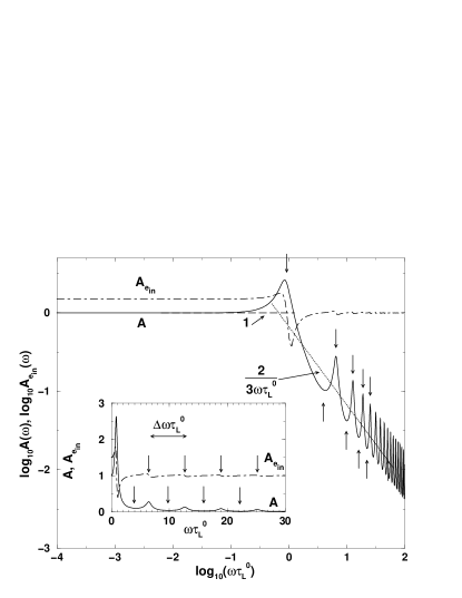
Figure 6: Amplitude $A$ of the response $\Delta(t)$ as a function of the driving frequency $\omega$ (log-log-scale) for weak modulations ($e_{f}=0.1$) of the driving force $f$, and $Re_{0}=10^{4}$. The time scale of the energy cascade is set to $\tau=a=1$. The dashed line denotes the low frequency limit of the oscillation amplitude, $1$, and the dotted line corresponds to the mean trend of the high frequency limit, $\frac{2}{3}\frac{1}{\omega\tau_{L}^{0}}$. The dashed-dotted line represents the amplitude of the resulting energy input rate $e_{in}(t)$. Inset: linear-scale-plot of the response amplitude (solid line) and the energy input amplitude (dashed-dotted line) versus frequency. The small arrows indicate the frequencies $\omega_{r}$ (in units of $\tau_{L}^{0}$) of the response extrema calculated from the extrema of the denominator in Eq. (33). The horizontal arrow denotes the frequency distance $\Delta\omega$ (in units of $\tau_{L}^{0}$) between two frequencies for which the amplitude is maximal (or minimal). It is $\Delta\omega\simeq 2\pi/\tau$ for high frequencies.

In Fig.6 the amplitude $A(\omega)$ of the response $\Delta$ is plotted as a function of driving frequency for $Re_{0}=10^{4}$. As for the modulated energy input rate we note that the amplitude remains constant for low frequencies and decreases as $\propto 1/\omega$ for high frequencies. Also the response maxima and minima can be observed. Quantitatively, the low frequency limit for a modulated forcing is different from the modulated energy input rate case. For low driving frequencies, $\omega\ll 1/\tau$, we can approximate Eq. (33) by:

$$\Delta(t)\simeq e_{f}\frac{\frac{2}{3\omega}(\frac{1}{\omega}\sin{(\omega(t+\tau))}-\frac{1}{3\omega}\sin{\omega t})}{(\frac{1}{\omega})^{2}+(\frac{1}{3\omega})^{2}-2\frac{1}{\omega}\frac{1}{3\omega}\cos\omega\tau}.$$ (34)

The terms $6/Re_{0}\ll 1$ have been omitted here for simplicity. In the limit $\omega\tau\rightarrow 0$, with $\sin{\omega\tau}\rightarrow 0$ and $\cos{\omega\tau}\rightarrow 1$, the amplitude $A$ of the response (cf. Eq. (16)) becomes equal to one instead of two thirds (cf. Eq. (18)) for a modulated energy input rate. The frequencies of the reponse maxima and minima are determined by the extrema of the denominator of the solution (33). They are slightly shifted as compared to the case with modulated energy input rate (Eq. (17)). The amplitude at the first maximum is smaller than in the case with modulated energy input rate, namely $A_{E}\simeq 2.7$. However, in the limit of very high driving frequencies, $\omega\gg\frac{1}{\tau}$, Eq. (33) can be approximated by Eq. (19), i.e., the response amplitudes of both cases become identical.

It was pointed out in the beginning of this section that, if we modulate the driving force, the energy input rate is not a controlled quantity, but can be considered as well as a response of the system. This has been measured in a recent experimental study by Cadot et al.Cadot et al. (2002). Within the mean-field theory the energy input rate for a modulated driving force can be calculated as:

$$\frac{e_{in}(t)}{e_{in,0}}=\sqrt{1+\Delta(t)}(1+e_{f}\sin\omega t),$$ (35)

where $e_{in,0}=\langle\!\langle D_{L,0}^{1/2}f_{0}\rangle\!\rangle$ is the stationary energy input rate for constant forcing without modulation. In order to extract the amplitude of the energy input rate, we fit it by a function of the form $\frac{e_{in}(t)}{e_{in,0}}=1+e_{f}A_{e_{in}}\sin(\omega(t+\phi))$. This is justified as long as the modulation amplitude $e_{f}$ is small, i.e., $e_{f}\ll 1$, because then $\Delta(t)$ is of the same order of magnitude as $e_{f}$ and Eq. (35) can be approximated by $\frac{e_{in}(t)}{e_{in,0}}-1\simeq{1\over 2}\Delta(t)+e_{f}\sin\omega t+O(\Delta^{2})$. The amplitude $A_{e_{in}}$ of the energy input rate is included in Fig.6 as a dashed-dotted line. For low driving frequencies, $\omega\ll{1\over\tau}$, the amplitude $A_{e_{in}}$ is nearly constant and is $3/2$, whereas for high frequencies it decreases and finally saturates at one. Also the response maxima can be observed in the energy input rate: At the same frequencies, where the response $\Delta$ shows amplitude maxima, we observe a maximum directly followed by a minimum in the amplitude of the energy input rate.

In conclusion, if the driving force instead of the energy input rate is modulated, the general behavior of the response in terms of the second order structure function on the larges scale remains the same, including the response maxima and minima. For low driving frequencies, the amplitude of the response becomes equal to the amplitude of the forcing. In addition, the energy input rate can be regarded as a different measure for the response of the system, which also shows the response maxima at frequencies connected with the energy cascade time scale $\tau$.

VI Conclusions

We calculated the response of isotropic and homogeneous turbulence to a weak modulation of the energy input rate $e_{in}$ within a mean-field theory. For low frequencies the system follows the input rate modulation whereas for high frequencies the amplitude of the response decreases $\propto 1/\omega$. Due to the intrinsic time scale of the system, the eddy-turnover time $\tau$, which also characterizes the energy transport time down the eddy cascade, there are certain frequencies, $\omega_{r}\simeq n{\pi\over\tau}$, where the amplitude of the response is either increased or decreased. At these frequencies the phase shift $\phi$ between the energy input rate and the response is $\phi_{r}\simeq 3\pi/2$. The response extrema occur when the eddy-turnover time is an even or odd multiple of half the modulation period $T/2=\pi/\omega$, respectively. In the case of response maxima, the energy dissipation rate and the response of the system are in phase. This can be understood as a very effective transport of energy through the system. At the amplitude minima, instead, the response of the system is strongly reduced. Then, the energy dissipation rate and the response are exactly anti-phased.

In the mean-field approach the fluctuations of the energy flow rate through the system and of the large eddy turnover time are neglected. In experiment or numerical simulation the fluctuations are however present. They may lead to broader and less pronounced response maxima, i.e., partly wash out the response maxima and minima.

With increasing modulation amplitude $e$ of the energy input rate the response maxima are expected to become more significant due to the better signal to fluctuation ratio. But remember that for higher modulation amplitudes $e$, the time scale of the eddy cascade, which enters into our model as a time delay, becomes time dependent. This as well could lead to less pronounced response maxima as discussed in section III.3.

A way to check if the characteristic feature of the response maxima and minima can still be well identified under the influence of fluctuations, would be to perform numerical simulations of the Navier Stokes Equation with a modulated driving. However, as not only high Reynolds numbers are needed to achieve fully developed, isotropic and homogeneous turbulence, but also the response as a function of time for a wide range of frequencies has to be calculated, the computational effort would be too high. Therefore, numerical simulations within two dynamical cascade models of turbulence, the GOY shell model Gledzer (1973); Yamada and Ohkitani (1987, 1988); Ohkitani and Yamada (1989); Jensen et al. (1991); Kadanoff et al. (1995); Biferale (2003) and the reduced wave vector set approximation (REWA) Eggers and Grossmann (1991); Grossmann and Lohse (1992, 1994), were performed von der Heydt et al. (2003). These models take into account the fluctuations. The basic trend of the frequency dependence of the response amplitude as calculated within the mean-field model can be reproduced in both numerical models. We also clearly find the main maximum in both models although it os of course washed out by the fluctuations. The higher maxima and minima however seem to be completely washed out.

Also a recent experimental study of modulated turbulence by Cadot et al. Cadot et al. (2002) showed evidence for the existence of the response maxima. This experiment may be comparable with our study of a modulated driving force as discussed in section V. The response maxima were measured in the amplitude of the energy input rate. In addition, a constant response amplitude for low driving frequencies and a $1/\omega$-decay of the velocity response amplitude for large frequencies has been observed. This is in agreement with the $1/\omega$-decay of the energy response amplitude which we have found in the mean-field model. The velocity response $(u(t)-u_{0})/u_{0}=\Delta_{u}(t)$, where $u(t)$ is the measured velocity modulus and $u_{0}$ the (stationary) mean velocity, is connected to the energy response $\Delta(t)$ which we have calculated in this paper by $1+\Delta(t)=u(t)^{2}/u_{0}^{2}=(1+\Delta_{u}(t))^{2}\simeq 1+2\Delta_{u}(t)+O(\Delta_{u}^{2})$. As only small modulation amplitudes are considered the term $+O(\Delta_{u}^{2})$ will be negligible because $\Delta_{u}\ll 1$. Therefore, the experimentally measured $1/\omega$-decay of the amplitude $\Delta_{u}$ of the velocity response is just what one would expect from our theoretical prediction $\Delta\propto 1/\omega$ for the amplitude of the energy response.

We hope that the present work will stimulate even more experimental and numercial studies on the role of the energy cascade time scale in modulated turbulence.

Acknowledgments: We thank R. Pandit and B. Eckhardt for very helpful discussions. The work is part of the research program of the Stichting voor Fundamenteel Onderzoek der Materie (FOM), which is financially supported by the Nederlandse Organisatie voor Wetenschappelijk Onderzoek (NWO). This research was also supported by the German-Israeli Foundation (GIF) and by the European Union under contract HPRN-CT-2000-00162.

References

- Rippeth et al. (2001) T. P. Rippeth, N. R. Fisher, and J. H. Simpson, J. Phys. Oceanogr. 31, 2458 (2001).
- Scotti and Piomelli (2001) A. Scotti and U. Piomelli, Phys. Fluids 13, 1367 (2001).
- Qiu et al. (2000) X. L. Qiu, S. H. Yao, and P. Tong, Phys. Rev. E 61, R6075 (2000).
- Qiu and Tong (2001a) X. L. Qiu and P. Tong, Phys. Rev. E 64, 036304 (2001a).
- Qiu and Tong (2001b) X. L. Qiu and P. Tong, Phys. Rev. Lett 87, 094501 (2001b).
- Labbé et al. (1996) R. Labbé, J. F. Pinton, and S. Fauve, Phys. Fluids 8, 914 (1996).
- Aumaître et al. (2000) S. Aumaître, S. Fauve, and J. F. Pinton, Eur. Phys. J. B 16, 563 (2000).
- Lohse (2000) D. Lohse, Phys. Rev. E 62, 4946 (2000).
- Hooghoudt et al. (2001) J. O. Hooghoudt, D. Lohse, and F. Toschi, Phys. Fluids 13, 2013 (2001).
- Effinger and Grossmann (1987) H. Effinger and S. Grossmann, Z. Phys. B 66, 289 (1987).
- Monin and Yaglom (1975) A. S. Monin and A. M. Yaglom, Statistical Fluid Mechanics (The MIT Press, Cambridge, Massachusetts, 1975).
- Sreenivasan (1995) K. R. Sreenivasan, Phys. Fluids 7, 2778 (1995).
- Sreenivasan and Antonia (1997) K. R. Sreenivasan and R. A. Antonia, Ann. Rev. of Fluid Mech. 29, 435 (1997).
- Pope (2000) S. B. Pope, Turbulent Flows (Cambridge University Press, Cambridge, 2000).
- Sreenivasan (1984) K. R. Sreenivasan, Phys. Fluids 27, 1048 (1984).
- Sreenivasan (1998) K. R. Sreenivasan, Phys. Fluids 10, 528 (1998).
- Lohse (1994) D. Lohse, Phys. Rev. Lett. 73, 3223 (1994).
- Grossmann (1995) S. Grossmann, Phys. Rev. E 51, 6275 (1995).
- Stolovitzky and Sreenivasan (1995) G. Stolovitzky and K. R. Sreenivasan, Phys. Rev. E 52, 3242 (1995).
- Rao et al. (1990) M. Rao, H. Krishnamurthy, and R. Pandit, Phys. Rev. B 42, 856 (1990).
- Cadot et al. (2002) O. Cadot, J. H. Titon, and D. Bonn, Preprint, submitted to J. Fluid Mech. (2002).
- Gledzer (1973) E. B. Gledzer, Sov. Phys. Dokl. 18, 216 (1973).
- Yamada and Ohkitani (1987) M. Yamada and K. Ohkitani, J. Phys. Soc. Jpn. 56, 4210 (1987).
- Yamada and Ohkitani (1988) M. Yamada and K. Ohkitani, Prog. Theor. Phys. 79, 1265 (1988).
- Ohkitani and Yamada (1989) K. Ohkitani and M. Yamada, Prog. Theor. Phys. 81, 329 (1989).
- Kadanoff et al. (1995) L. Kadanoff, D. Lohse, J. Wang, and R. Benzi, Phys. Fluids 7, 617 (1995).
- Biferale (2003) L. Biferale, Ann. Rev. Fluid Mech. 35, 441 (2003).
- Jensen et al. (1991) M. H. Jensen, G. Paladin, and A. Vulpiani, Phys. Rev. A 43, 798 (1991).
- Grossmann and Lohse (1994) S. Grossmann and D. Lohse, Phys. Fluids 6, 611 (1994).
- Eggers and Grossmann (1991) J. Eggers and S. Grossmann, Phys. Fluids A 3, 1958 (1991).
- Grossmann and Lohse (1992) S. Grossmann and D. Lohse, Z. Phys. B 89, 11 (1992).
- von der Heydt et al. (2003) A. von der Heydt, S. Grossmann, and D. Lohse, Preprint, submitted to Phys. Rev. E (2003).