Stabilization of solitons of the multidimensional nonlinear Schrödinger equation: Matter-wave breathers

Abstract

We demonstrate that stabilization of solitons of the multidimensional Schrödinger equation with a cubic nonlinearity may be achieved by a suitable periodic control of the nonlinear term. The effect of this control is to stabilize the unstable solitary waves which belong to the frontier between expanding and collapsing solutions and to provide an oscillating solitonic structure, some sort of breather-type solution. We obtain precise conditions on the control parameters to achieve the stabilization and compare our results with accurate numerical simulations of the nonlinear Schrödinger equation. Because of the application of these ideas to matter waves these solutions are some sort of matter breathers.

, ,

1 Introduction

The nonlinear Schrödinger equation (NLSE) in its many versions is one of the most important models of mathematical physics, with applications to different fields such as plasma physics, nonlinear optics, water waves and biomolecular dynamics, to cite only a few cases. In many of those examples the equation appears as an asymptotic limit for a slowly varying dispersive wave envelope propagating in a nonlinear medium [1, 2].

A new burst of interest on problems modelized by nonlinear Schrödinger equations has been triggered by the achievement of Bose-Einstein condensation using ultracold neutral bosonic gases [3, 4].

In particular in Bose-Einstein condensation one of the key ingredients of the achievement of condensation with alkali gases is the trapping of the neutral atoms which are cooled down below the transition temperatures. Although different trapping techniques have been used in practice, the most commonly used are the magnetic traps which are modelized by external confining forces acting on the system.

There are specific types of Bose-Einstein condensates such as those made of Lithium [5, 6] in which the interactions between the atoms are attractive. Mathematically this implies that for spatial dimensionalities $n=2,3$ collapsing solutions are possible as it is well known in the framework of the usual studies of nonlinear Schrödinger equations [2]. Thus, although in principle one could think that nonlinearity and dispersion could balance mutually and a self-sustained solitonic structure might exist this is only true for $n=1$. In fact, it was soon found experimentally [5, 6] and theoretically supported that such a situation is unstable and leads to collapse [2, 7]. Later studies, taking into account more elaborate models than the simpler NLS mean field models, led to the understanding that the occurrence of collapse during the condensation process would limit the size of an attractive condensate [9, 10].

Thus, the only confirmed way to observe solitonic states in Bose-Einstein condensates (matter-wave solitons) with negative scattering length involves the elimination of the trap in one direction as proposed in [11, 12] and found experimentally in [13, 14].

However, the possibility of using Feschbach resonances to control the scattering length [15, 16, 17] has provided a way to study large negative scattering length condensates and collapse processes in detail [18, 19]. This control allows, with certain experimental limitations, to modulate appropriately the nonlinear term.

But this possibility opens new ways for the generation and observation of different types of matter-wave solitons not yet fully explored. One of the most striking ones is the possibility of generating trapless trapped Bose-Einstein condensate solitons. The idea is that (oscillating) bound states might be obtained by combining cicles of positive and negative scattering length values so that after an expansion and contraction regime the condensate would come back to the initial state. In this way some sort of pulsating trapped condensate, i.e., a breather, would be obtained.

A rigorous study of this intuitive idea is necessary in order to make precise predictions and find which are the precise parameter values to be used to obtain such breathers. This is the purpouse of this paper in a general framework of nonlinear Schrödinger systems. This idea has been explored in two previous papers [20, 21] but here we improve the understanding of the phenomenon and correct mistakes contained in the previous analysis.

Another field of applications of these ideas is nonlinear Optics, there a full control of the nonlinear term is not possible but, because of technical limitations, only piecewise constant values for the nonlinear coefficient can be easily generated experimentally.

¿From the mathematical point of view what we would like is to stabilize solutions close to the stationary unstable solitons of the cubic NLSE by choosing appropriate controls of the nonlinear term. To our knowledge this problem has not been considered previously in the mathematical literature.

This paper is organized as follows: First, in Sec. 2 we present the model equations as they appear in one specific application of the model. Next, in Sec. 3 we reduce the nonlinear model to a system of ordinary differential equations by using the so-called moment method. In Sec. 4 we analyze two-dimensional systems and compare the analytical predictions of the moment method with numerical simulations of the full partial differential equations. We obtain precise conditions for the existence of breathers and discuss the importance of the initial data. In Sec. 5 we analyze the three-dimensional case and explain why moment (or related) equations fail to describe the dynamics of the spherically symmetric case. We consider the case of systems in specific external potentials and give some stabilization conditions. Finally, in Sec. 6 we summarize our conclusions and compare our results with the previous findings of Refs. [20, 21].

2 The model

In this work we study systems ruled by the NLSE with a cubic nonlinearity. In the framework of recent problems in Bose-Einstein condensation this equation appears as the model for the mean field dynamics of a boson system described by a single wavefunction $\Psi$ in the zero–temperature limit. The resulting NLSE equation is called sometimes the Gross–Pitaevskii equation (GPE) which is [22]

$$i\hbar\frac{\partial\Psi}{\partial\tau}=\left[-\frac{\hbar^{2}}{2m}\triangle+V({\bf r})+\frac{4\pi a\hbar^{2}}{m}|\Psi|^{2}\right]\Psi,$$ (1)

where $\triangle=\sum_{j=1}^{3}\partial^{2}/\partial r_{j}^{2}$ is the three-dimensional Laplacian, $V({\bf r})=\frac{1}{2}m\omega^{2}\sum_{j=1}^{3}\lambda_{j}^{2}r_{j}^{2}$ is the external potential (the so called “trap”) which confines the condensate and $a$ is the $s$–wave scattering length for the binary collisions within the condensate.

It is more convenient to work with a new set of adimensional quantities defined as $x_{j}=r_{j}/a_{0},t=\tau/T$, $\psi({\bf x},t)\equiv\Psi({\bf r},\tau)\sqrt{a_{0}^{3}/N}$, where $a_{0}=\sqrt{\hbar/m\omega}$, $T=1/\omega$ and $N=\int|\Psi|^{2}d^{3}r$ is the number of particles in the condensate. Then Eq. (1) reads as the next NLSE

$$i\frac{\partial\psi}{\partial t}=\left[-\frac{1}{2}\triangle+\frac{1}{2}\sum_{j=1}^{3}\lambda_{j}^{2}x_{j}^{2}+g|\psi|^{2}\right]\psi,$$ (2)

where $g=4\pi Na/a_{0}$ and $\int|\psi|^{2}d^{3}x=1$. In this paper we consider a system evolving without external potential along one or more dimensions. In Bose-Einstein condensation this corresponds to a condensate generated in a trap and then the trapping is eliminated. This leads to different particular cases of Eq. (2). When the potential is removed in all directions we obtain

$$i\frac{\partial\psi}{\partial t}=\left[-\frac{1}{2}\triangle+g|\psi|^{2}\right]\psi.$$ (3)

This equation holds for three-dimensional and quasi two-dimensional systems as will be discussed in detail in Sec. 5. Eq. (3) has the typical form of the NLSE with cubic power nonlinearity [2] and has been extensively studied. In this work we will analyze the possibilities of controlling the behavior of the stationary solutions of Eq. (3) by letting $g$ be a time-dependent real function. Similar possibilities for nonconstant $g$ (in that context z $\leftrightarrow$ t) but restricted to $n=2$ arise in the context of coherent light propagation in nonlinear Kerr media in the paraxial approximation.

3 Moment method

In this section we build a theory which will allow us to reduce the dynamics from the complex model given by Eq. (3) to a simpler one whose analysis will provide insight on the basic features of the phenomenon.

Let us first consider radially symmetric solutions of Eq. (3) $u=u(r,t)$, $r=(\sum_{j=1}^{n}x_{j})^{1/2}$, satisfying

$$i\frac{\partial u}{\partial t}=-\frac{1}{2r^{n-1}}\frac{\partial}{\partial r}\left(r^{n-1}\frac{\partial u}{\partial r}\right)+g(t)|u|^{2}u.$$ (4)

where $n$ is the spatial dimensionality, in our case $n=2,3$. To get information on the solutions of Eq. (4) we will use the moment method [23, 24, 25, 26, 27]. This method proceeds by analyzing the evolution of several integral quantities [23, 24, 25] related with Eq. (4).

$$I_{1}(t) = \int|u|^{2}d^{n}x$$ (5a)

$$I_{2}(t) = \int|u|^{2}r^{2}d^{n}x,$$ (5b)

$$I_{3}(t) = i\int\left(u\frac{\partial u^{*}}{\partial r}-u^{*}\frac{\partial u}{\partial r}\right)\!r\ d^{n}x,$$ (5c)

$$I_{4}(t) = \frac{1}{2}\int\left(\left|\nabla u\right|^{2}+\frac{n}{2}g(t)|u|^{4}\right)d^{n}x,$$ (5d)

$$I_{5}(t) = \frac{n}{4}\int|u|^{4}d^{n}x,$$ (5e)

where $d^{n}x=r^{n-1}drd\Omega$. With our scaling for $\psi$, the first one satisfies $I_{1}=1$, for all $t$. The remaining ones are related physically to the width, radial momentum and energy of the wave packet. In what follows we assume that the initial data are such that all $I_{j}$ are initially well-defined [28]. Some algebra leads to

$$\frac{dI_{2}}{dt} = I_{3},$$ (6a)

$$\frac{dI_{3}}{dt} = 4I_{4},$$ (6b)

$$\frac{dI_{4}}{dt} = g\frac{n-2}{n}\frac{dI_{5}}{dt}+\frac{dg}{dt}I_{5},$$ (6c)

$$\frac{dI_{5}}{dt} = \frac{n\pi 2^{n}}{8}\int\frac{\partial|u|^{4}}{\partial r}\frac{\partial\arg u}{\partial r}r^{n-1}dr\simeq-\frac{nI_{3}I_{5}}{2I_{2}}.$$ (6d)

All the momenta follow closed evolution laws except for $I_{5}(t)$. In specific situations the moment equations provide completely closed equations for the evolution of all the $I_{j}$ [25, 27, 28] but this is not our case. Extending the number of momenta which are included in the calculation does not help to obtain a closed set of equations.

Thus, to close the system we will take

$$\arg u=I_{3}r^{2}/4I_{2},$$ (7)

as used in [26]. Physically, this corresponds to approximating the phase of $u$ by the spherical wavefront which best fits the distribution. A rigorous justification of this choice is possible [8] for the case $n=2$ and when the initial data is the so-called Townes soliton to be presented later.

When solutions with phase given by Eq. (7) are considered Eqs. (6) are closed and have several (positive) invariants under time evolution given by

$$Q_{1} = 2(I_{4}-gI_{5})I_{2}-I_{3}^{2}/4,$$ (8a)

$$Q_{2} = 2I_{2}^{n/2}I_{5}.$$ (8b)

With the help of these quantities, Eqs. (6) can be reduced to a single equation for $I_{2}(t)$, which is

$$\frac{d^{2}I_{2}}{dt^{2}}-\frac{1}{2I_{2}}\left(\frac{dI_{2}}{dt}\right)^{2}=2\left(\frac{Q_{1}}{I_{2}}+g\frac{Q_{2}}{I_{2}^{n/2}}\right).$$ (9)

If we were able to solve Eq. (9) then the use of Eqs. (6) would allow us to track the evolution of the other ones. To simplify Eq. (9) we define $X(t)=\sqrt{I_{2}(t)}$, which is the wave packet width, and substituting it into (9) we get

$$\ddot{X}=\frac{Q_{1}}{X^{3}}+g(t)\frac{Q_{2}}{X^{n+1}}.$$ (10)

4 Two-dimensional systems

4.1 Rigorous analysis of the moment equations

In physical situations both problems with $n=2$ and $n=3$ arise. The situation when a Bose-Einstein condensate is tightly confined along a particular direction leads to a quasi two-dimensional system such as the ones obtained in Ref. [29]. From now on we consider the two-dimensional model to be valid in that situation although a more detailed analysis will be made in Sec. 6. Thus, when $n=2$ we obtain

$$\ddot{X}=\frac{Q_{1}+Q_{2}g(t)}{X^{3}}\equiv\frac{p(t)}{X^{3}}.$$ (11)

This equation appears also in relation with the classical motion of an atom near an infinite straight wire with oscillating charge (the Paul trap) [30, 31, 32] and also as an approximate model for beam propagation in layered Kerr media [33].

Let us consider the case where $p$ is continuous and $T$-periodic and look for positive periodic solutions and bound states, that is, bounded (nonperiodic) positive solutions without collapse. If $p(t)\geq 0$ all solutions escape to infinity whereas if $p(t)<0$ all solutions collapse. In fact, theorem 2.1 of [31] implies that a necessary condition for existence of bound states is

$$\overline{p}=\frac{1}{T}\int_{0}^{T}p<0.$$ (12)

Let $p(t)$ be parametrized as $p(t)=\alpha+\beta a(t)$ with $\overline{a}=0$. We can fix $a_{M}=\max a(t)=1$ without loss of generality. A direct consequence of the latter result is that if $\alpha\geq 0$ bound states cannot exist, therefore $\alpha$ must be negative. Also, $p(t)$ must change sign, so for existence of bound states it is necessary that

$$\alpha+|\beta|>0.$$ (13)

Let us introduce the positive small parameter $\epsilon=-2\alpha/3|\beta|$. We will now prove that there exists $\epsilon_{0}>0$ (depending only on $a$) such that Eq. $(\ref{singular2D})$ has a Lyapunov-stable periodic solution if $0<\epsilon<\epsilon_{0}$. Moreover, there is an infinite number of quasiperiodic solutions and a sequence of subharmonics with minimal periods tending to $+\infty$. To prove this affirmation let us note that when $a(t)=\cos\Omega t$, Theorem 1 in [32] asserts that if $\epsilon$ is small enough there is a periodic solution of twist type [34]. However, the proof is still valid for a general continuous and $T$-periodic function with $\overline{a}=0$. Moser Twist Theorem [35] implies that a solution of twist type is Lyapunov-stable as a consequence of the existence of invariant curves (quasiperiodic solutions) around it. Finally, the existence of subharmonics of any order is a consequence of Poincare-Birkhoff Theorem.

This result has interesting physical consequences. The existence of periodic solutions is directly related to the existence of pulsating breathers. The bounded solutions of the theorem would correspond to solutions with quasiperiodic or chaotic oscillations in the width. In fact, Mather sets and Smale’s horseshoes appear in the Poincaré map. The latter correspond to chaotic oscillations whereas Mather sets are Cantorian structures that are more complicated than the quasiperiodic ones.

We have just seen that a necessary condition for the existence of bounded solutions is that $\alpha+|\beta|>0$ with $\alpha<0$. Moreover the previous result indicates that the amplitude of the oscillating term must be of the same order as the amplitude of the non-oscillating term.

To find particular types of these breathers let us take $g(t)$ as $g(t)=g_{0}+g_{1}\cos(\Omega t)$ so that $p(t)=\alpha+\beta\cos(\Omega t)$ with $\alpha=Q_{1}+g_{0}Q_{2}$ and $\beta=g_{1}Q_{2}$. An useful tool to get periodic solutions is the stability diagram of Eq. (11). We look for the region of parameters for which there exist stable periodic solutions. To do this we reduce the number of parameters by defining a new time as $\tilde{t}=\Omega t$. Then Eq. (11) is

$$X^{\prime\prime}=\frac{\tilde{\alpha}+\tilde{\beta}\cos(\tilde{t})}{X^{3}},$$ (14)

where the prime denotes derivative with respect to $\tilde{t}$, $\tilde{\alpha}=\alpha/\Omega^{2}$ and $\tilde{\beta}=\beta/\Omega^{2}$. Note that we use the word stable with two different meanings: the more mathematical one to indicate Lyapunov-stability and the more physical one to indicate existence of periodic solutions of the nonlinear Schrödinger equation.

Our objective is to find the region of parameters ($\tilde{\alpha}$,$\tilde{\beta}$) in which there exist initial conditions $X_{0}=X(\tilde{t}=0)$, $X_{0}^{\prime}=X^{\prime}(\tilde{t}=0)=0$ for which Eq. (14) has a stable periodic solution. We already know that our search can be restricted to the region given by the conditions $\tilde{\alpha}<0$ and $\tilde{\alpha}>-|\tilde{\beta}|$. To calculate the stabilization region we first solve numerically Eq. (14). Then we take into account the results that finding a periodic solution of Eq. (14) is equivalent to finding a solution which verifies the Neumann conditions $X^{\prime}(0)=0=X^{\prime}(2\pi)$. The reason is that by extending in an even way this solution, we obtain a 4$\pi$-periodic solution that, of course, is bounded and periodic and this implies that there is a $2\pi$-periodic solution [36]. To obtain solutions that verify the Neumann conditions, given a pair of parameters ($\tilde{\alpha}$,$\tilde{\beta}$), we look for two initial conditions $X_{1,0}$ and $X_{2,0}$ for which $X_{1}^{\prime}(2\pi)X_{2}^{\prime}(2\pi)<0$. Then, by continuity with respect to the initial conditions it is known that there exists one initial condition $X_{0}$, between $X_{1,0}$ and $X_{2,0}$, for which the solution of the equation satisfies $X^{\prime}(2\pi)=0$. We will use two more observations. First of them is that if $X(\tilde{t})$ is a solution of the equation with parameters ($\tilde{\alpha}$,$\tilde{\beta}$), then $Y(\tilde{t})=cX(\tilde{t})$ with $c$ any arbitrary positive constant is also a solution with parameters ($\tilde{\alpha}c^{4}$,$\tilde{\beta}c^{4}$). Therefore, by moving $c$, all the points of the line $y=(\tilde{\beta}/\tilde{\alpha})x$ are obtained and this is nothing but the line which passes through the points ($\tilde{\alpha}$,$\tilde{\beta}$) and $(0,0)$. So, to scan the region of parameters we can, for example, to pay attention to an specific value of $\tilde{\alpha}$ and then change continuosly the parameter $\tilde{\beta}$. The second observation is that if $X(\tilde{t})$ is a periodic solution corresponding to a specific choice of ($\tilde{\alpha}$,$\tilde{\beta}$) then $Y(\tilde{t})=X(\tilde{t}+\pi)$ is also a solution for parameters ($\tilde{\alpha}$,-$\tilde{\beta}$) since $\cos(\tilde{t}+\pi)=-\cos(\tilde{t})$. Therefore, the stability region is symmetric and we can restrict the search to $\tilde{\beta}>0$. With all these considerations the results obtained show that the region of parameters for which there exist initial conditions leading to stable periodic solutions is given by Eq. (13) so this condition seems to be not only necessary but also a sufficient one. In Fig. 1 this stability region is plotted.

Figure 1: Stability diagram for Eq. (14) as a function of the parameters ($\tilde{\alpha}$,$\tilde{\beta}$).

4.2 Comparison with full numerical simulations of the NLSE

In this subsection we will compare the predictions based on the ordinary differential equation (11) with the simulations of the full nonlinear Schrödinger equation (3).

First of all we have to choose appropriate initial data $u_{0}=u(r,t=0)$ in order to solve numerically the NLSE. Since we are going to try to stabilize the solutions it is reasonable to start trying to stabilize the so-called stationary solutions. So, let us consider stationary solutions of Eq. (3) when $g=g_{s}$ is constant, given by $u(\textbf{x},t)=e^{i\mu t}\Phi_{\mu}(\textbf{x})$. Here $\Phi_{\mu}(\textbf{x})$ verifies

$$\triangle\Phi_{\mu}-2\mu\Phi_{\mu}-2g_{s}|\Phi_{\mu}|^{2}\Phi_{\mu}=0.$$ (15)

As it is precisely stated in [2], when $g_{s}$ is negative, for each positive $\mu$ there exists only one solution of Eq. (1) which is real, positive and radially symmetric and for which $(\int|\Phi_{\mu}|^{2}d^{n}x)^{1/2}$ has the minimum value between all of the possible solutions of Eq. (15). Moreover, the positivity of $\mu$ ensures that this solution decays exponentially at infinity. This solution is called the ground state and, in two dimensions, is known as the Townes soliton. We will denote this solution as $R_{\mu}(r)$ and satisfies the equation

$$\triangle R_{\mu}-2\mu R_{\mu}-2g_{s}R_{\mu}^{3}=0$$ (16)

and the boundary conditions

$$\lim_{r\rightarrow{\infty}}R_{\mu}(r)=0,\ R_{\mu}^{\prime}(0)=0.$$ (17)

Fixed a value of $\mu$, the norm and width of $R_{\mu}$ are given by $\eta_{\mu}=(\int|R_{\mu}|^{2}d^{2}x)^{1/2}$ and $X_{\mu}=(\int|R_{\mu}|^{2}r^{2}d^{2}x)^{1/2}$ respectively. Applying scaling trasformations to $R_{\mu}(r)$ it is possible to build stationary solutions having the same shape and norm as the Townes soliton but different widths

$$R_{\mu}(r)=\mu^{1/2}R_{1}(\mu^{1/2}r),\ X_{\mu}=X_{1}/\mu^{1/2}.$$ (18)

The equation which verifies the normalized soliton $R_{\mu,N}(r)=R_{\mu}(r)/\eta_{\mu}$ is

$$\triangle R_{\mu,N}-2\mu R_{\mu,N}-2g_{s}\eta_{\mu}^{2}R_{\mu,N}^{3}=0.$$ (19)

We have taken as initial condition $u(r,t=0)=R_{\mu,N}(r)$ for some $\mu$ (therefore the initial width is fixed) and $g_{s}$ values. To obtain the shape $R_{\mu}(r)$ we have used a shooting method [37] to solve Eq. (16). The idea is to rewrite Eq. (16) as a dynamical system and impose that the solution of such a system also verifies the boundary conditions (17). In order to avoid the singularity which appears at the point $r=0$ we have solved the indetermination by means of a series expansion of $R_{\mu}$ around $r=0$.

¿From the theory of nonlinear Schrödinger equations it is known that the Townes soliton is unstable, i.e. small perturbations of this solution lead to either expansion of the initial data or blow-up in finite time. Thus, following the analogy with the stabilization of unstable fixed points in finite dimensional dynamical systems by fast variation of a parameter, we will try to stabilize this unstable but anyway stationary solution of Eq. (3).

Using the predictions of Eq. (11), in order to get stable periodic solutions, we have to choose $g_{0}$ such that $\alpha=Q_{1}+g_{0}Q_{2}$ is negative, that is, the following relation must hold

$$g_{0}<-\frac{\int|\nabla u_{0}|^{2}d^{2}x}{\int|u_{0}|^{4}d^{2}x}.$$ (20)

When only such a $g_{0}$-term is present the solutions collapse as predicted by Eq. (11). So, the $g_{1}$-term is necessary in order to arrest the collapse and achieve the stabilization of the soliton given by $u_{0}$.

Thus, we have first taken as initial data the Townes soliton obtained for $g_{s}=-0.5$ and $\mu=0.5$ whose width is $X_{0}=1.09$ and its norm satisfies $g_{s}\eta_{\mu=0.5}^{2}=-5.85$. This value is precisely the critical nonlinearity for collapse below which the collapse occurs. Let us note that only for the Townes soliton it is satisfied that the collapse threshold in Eq. (3), when $g$ is a constant, is just the value of the nonlinearity in Eq. (19) [2, 8].

In all the simulations of Eq. (3) we have made there appear two different types of behaviors. First, there is a small-amplitude fast oscillation due to the term $\cos(\Omega t)$ which is present in both the full model Eq. (3) and the reduced ODE system. Secondly, there is a “slow” dynamics due to the internal dynamics of the system which sometimes does not appear in the ODE model. When the results from the ODE (11) and the full PDE are compared qualitatively similar dynamics are observed in many situations. For instance, in Fig. 2 we plot the results of the simulation for parameter values $g_{0}=-2\pi$, $g_{1}=8\pi$ and $\Omega=40$. To solve numerically Eq. (3) we have used a pseudo-spectral method combined with a second order split-step method to advance in time [38, 39, 40]. We have also compared this simulation with the one obtained with a fourth order split-step method and found both results in full agreement.

It is important to indicate that it is absolutely necessary to incorporate an absorbing potential at the frontier of the simulation region to avoid possible interferences between the fraction of the wave packet moving outside (i.e. a possible non-trapped fraction of initial data) and the fraction of the initial data which remains trapped. Typical grid sizes were $256\times 256$ and the time step was $dt=0.001$. All results were tested on different grid sizes and changing time steps.

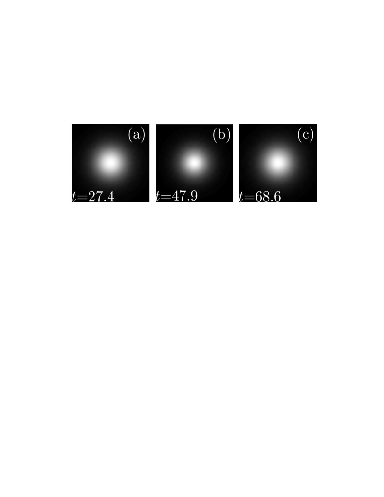
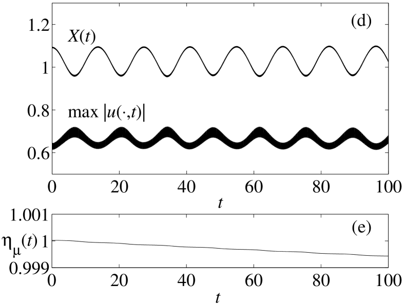
Figure 2: Results of numerical simulations of Eq. (3) showing stabilization of the initial data $u({\bf x},0)=R_{\mu,N}({\bf x})$ with $\mu=0.5$ and $g_{s}=-0.5$ ($X_{0}=1.09$) for parameter values $g_{0}=-2\pi$, $g_{1}=8\pi$, $\Omega=40$. (a-c) Plots of $|u({\bf x},t)|^{2}$ on the spatial region $[-2,2]\times[-2,2]$ corresponding to times of maximum (a,c) and minimum (b) width of the solution. (d) Evolution of the width $X(t)$ and of the amplitude $\max|u(\cdot,t)|$. (e) Evolution of the norm $\eta_{\mu}(t)$.

Clearly, the system is trapped with a fast modulation in the nonlinearity ($g_{1}$-term) and the collapse process is inhibited. Also, there is a fast oscillation with the same frequency $\Omega$ as the one of the oscillating term, (beyond the resolution of the plot), and a slow oscillation due to the proper dynamics of the system.

In Fig. 2(e) it is observed that the norm of the solution decreases in time. This is caused by the action of the absorbing potential on the outgoing way.

The next step in our study is to compare this stabilization in the NLSE with the differential equation for the width. In Fig. 3 we see that the quantitative predictions of Eq. (11) are not very precise as what concerns the amplitude and frequency of the slow oscillation. In any case, at least the simple ODE model predicts correctly the trapping of the solution for these parameters. These results imply that the predictions of the ODE system must be taken only as qualitative indications of the possible dynamics.

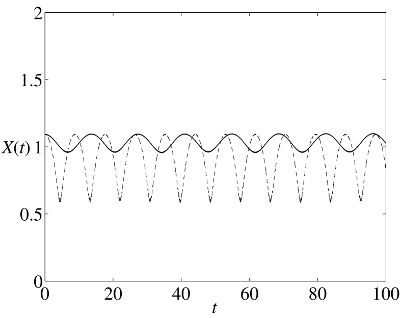
Figure 3: Results of numerical simulations of Eq. (3) and Eq. (11) showing stabilization of the initial data $u({\bf x},0)=R_{\mu,N}({\bf x})$ with $\mu=0.5$ ($X_{0}=1.09$) and $g_{s}=-0.5$ for parameter values $g_{0}=-2\pi$, $g_{1}=8\pi$, $\Omega=40$. The evolution of the width $X(t)$ according to Eq. (3) (solid) and to Eq. (11) (dashed) is shown.

Also, there exist parameter ($g_{0}$, $g_{1}$ and $\Omega$) choices which lead to stabilization in Eq. (11) but not in Eq. (3). For example, according to Eq. (11) and the diagram of Fig. 1 the parameters $g_{0}=-6.4$, $g_{1}=33.4$ and $\Omega=20$ stabilize the initial soliton as shown in Fig. 4. However, this stabilization does not happen when we solve numerically Eq. (3), instead, after a few oscillations their dynamics are drastically different.

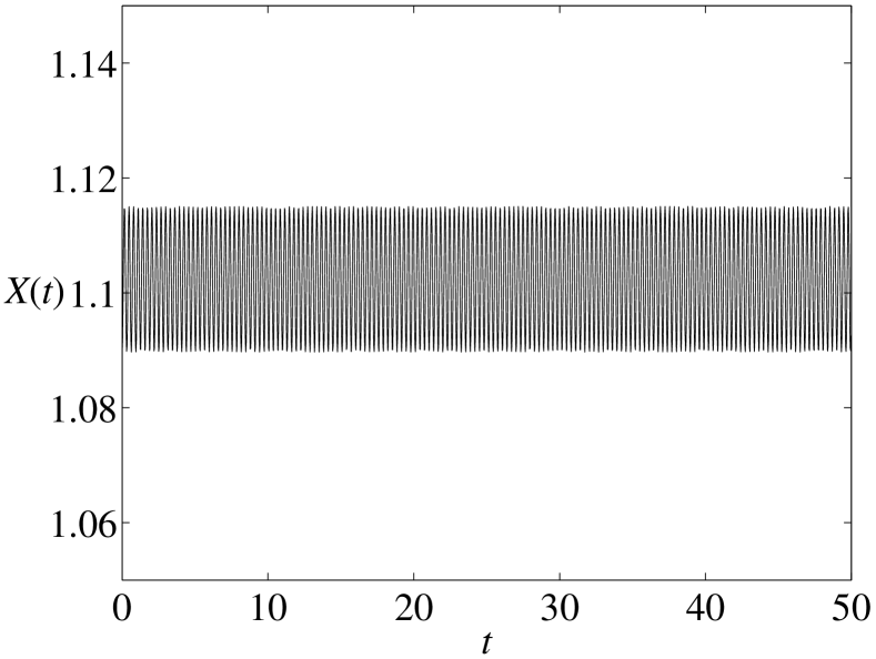
Figure 4: Results of numerical simulations of Eq. (11) showing stabilization of the initial data $u({\bf x},0)=R_{\mu,N}({\bf x})$ with $\mu=0.5$ and $g_{s}=-0.5$ ($X_{0}=1.09$) for parameter values $g_{0}=-6.4$, $g_{1}=33.4$, $\Omega=20$. The evolution of the width $X(t)$ is plotted.

4.3 Stabilization of other initial data

Although a Townes soliton is a natural object to stabilize in the framework of Eq. (3) we may wonder (i) if the procedure described above does stabilize other type of initial data and (ii) if the stabilization is appropriately described by Eqs. (11).

From the point of view of applications of Bose-Einstein condensation the possibility of stabilizing other initial data is important since it is not clear how a Townes soliton could be generated in real experiments. On the other hand, other initial data such as Thomas-Fermi type solutions or gaussians are much more natural and easier to obtain. This, together with the fact that the usual time dependent variational method [12] is usually developed for gaussian profile functions has lead to some interest on the possibility of trapping gaussian initial data (which is the case studied in Refs. [20, 21]).

Therefore, let us take $u_{0}$ as

$$u_{0}(r)=\frac{e^{-r^{2}/2X_{0}^{2}}}{\sqrt{\pi}X_{0}},$$ (21)

for which

$$\eta = \left(\int|u_{0}|^{2}d^{2}x\right)^{1/2}=1,$$ (22a)

$$X_{0} = \left(\int|u_{0}|^{2}r^{2}d^{2}x\right)^{1/2}.$$ (22b)

In this case we get for the invariants the values $Q_{1}=1$ and $Q_{2}=1/2\pi$ independently of the width $X_{0}$. So, the equation for the width is

$$\ddot{X}=\frac{1+g(t)/2\pi}{X^{3}}\equiv\frac{p(t)}{X^{3}}.$$ (23)

which corresponds to the evolution equation of Refs. [20, 21]. When $g$ is a constant this equation predicts a threshold value for collapse of $g=-2\pi$ which is, indeed, below the real value which corresponds to the Townes soliton ($g_{s}\eta_{\mu}^{2}=-5.85$). This means that when a Gaussian function is taken as initial data, Eq. (23) does not describe accurately the region of trapping, because for $-2\pi<g_{0}<-5.85$ this equation predicts expansion of the initial data while the real dynamics of the partial differential equation is collapsing.

In Fig. 5 the evolution of a Gaussian with $X_{0}=1.09$ and parameter values $g_{0}=-2\pi$, $g_{1}=8\pi$ and $\Omega=40$ is shown. Notice that these are the same width and parameters which allow trapping of a Townes soliton.

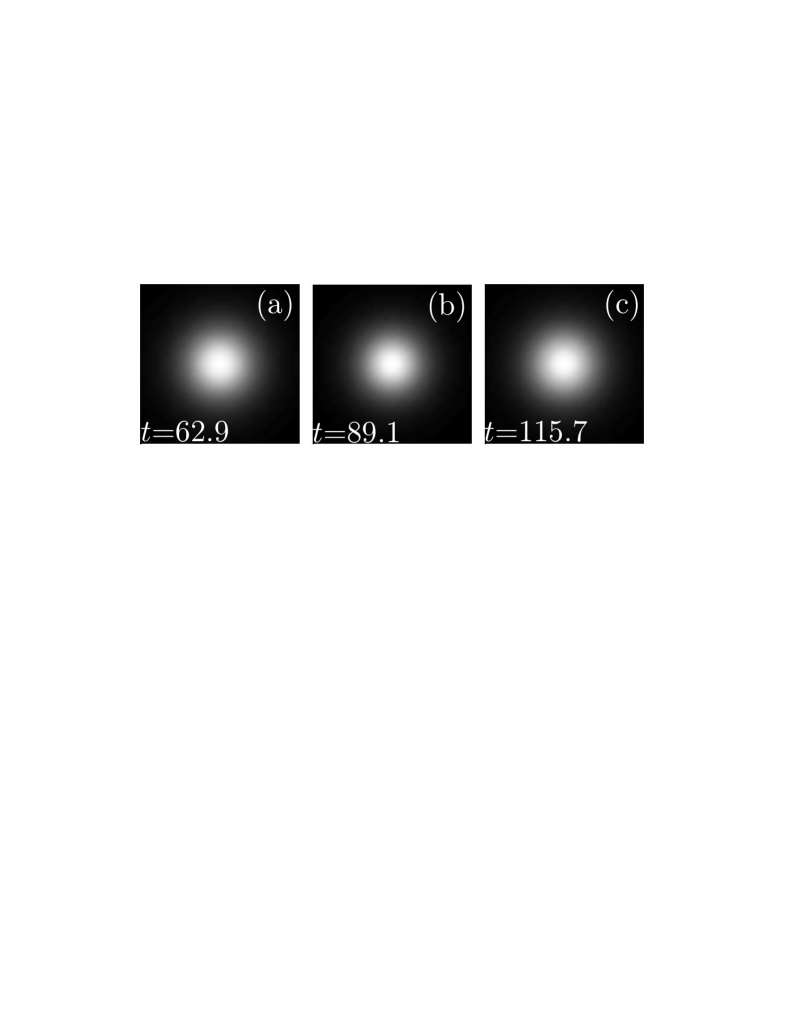
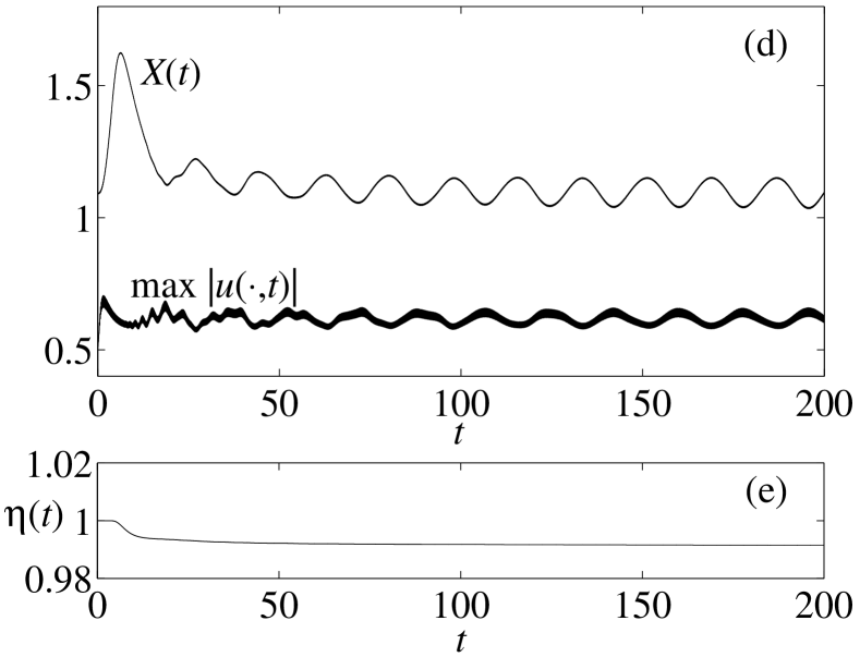
Figure 5: Results of numerical simulations of Eq. (3) showing stabilization of Gaussian initial data $u({\bf x},0)=(1/\sqrt{\pi}X_{0})e^{-r^{2}/2X_{0}^{2}}$ with $X_{0}=1.09$ for parameter values $g_{0}=-2\pi$, $g_{1}=8\pi$, $\Omega=40$. (a-c) Plots of $|u({\bf x},t)|^{2}$ on the spatial region $[-2,2]\times[-2,2]$ corresponding to times of maximum (a,c) and minimum (b) width of the solution. (d) Evolution of the width $X(t)$ and of the amplitude $\max|u(\cdot,t)|$. (e) Evolution of the norm $\eta(t)$.

We can see that with these parameters the stabilization is achieved although Eq. (23) does not predict trapping (in fact for these parameters $\bar{p}=0$). What is the difference with the stabilization of the Townes soliton shown in Fig. 2?. A first important observation is that in the case of Gaussian initial data a readjustment is produced soon by ejecting a significant part of the wave packet far from the trapping region. This corresponds to the first 10 time units where the width significantly increases due to the contribution of the outgoing wave. When this wave hits the absorbing region it is dissipated leading to the step in the norm evolution shown in Fig. 5(e). What remains trapped is indeed a Townes soliton.

Thus, the use of initial data different from a Townes soliton leads to a splitting of the solution into the soliton itself, which is the structure which can be stabilized, plus a certain amount of radiation which goes far from the region of interest. Because of this fact one must be careful to eliminate the outgoint part of the radiation in the numerical simulations. We have verified that when the absorbing region is absent the numerical simulations are misleading and the trapping effects are drastically altered (in fact, when zero boundary conditions at a given distance are used, there appear reflections in the boundary and essential changes on the results take place which would lead to spurious destabilization of the system after very short trapping times).

It is known that Eq. (3) with a cubic nonlinearity and two spatial dimensions corresponds to the so-called critical case [2, 8] in which diffraction and self-focusing are nearly balanced and collapse is extremely sensitive to perturbations and to changes in the initial conditions. For this reason although Gaussians look roughly like the Townes soliton they are not able to capture the delicate balance between diffraction and nonlinear focusing present in this case. When a Townes soliton is taken as a initial condition in Eq. (3) there is only a very small outgoing component which spreads out (due to numerical errors) and the system responds to the parametric perturbation as a whole. This fact implies that the moment equations may describe reasonably well the dynamics of the system only near the Townes soliton, since they only deal the global dynamics of the system. However, when the initial condition is a Gaussian, the component which spreads out cannot be captured neither by a moment-type formalism nor by the usual variational methods.

5 Three-dimensional systems

5.1 Analysis of the moment equations

Let us now consider the case $n=3$, then Eq. (10) reads

$$\ddot{X}=\frac{Q_{1}}{X^{3}}+g(t)\frac{Q_{2}}{X^{4}}.$$ (24)

Let us first assume that $g$ is continuous and $T$-periodic, then if $\overline{g}=\frac{1}{T}\int_{0}^{T}g\geq 0$ bound states cannot exist. The reason is that, by Massera theorem, a bound state would imply the existence of a periodic solution. But if there is a periodic solution $X$, multiplying $(\ref{singular3D})$ by $X^{4}$ and integrating over a period we get $0>-4\int_{0}^{T}X^{3}\dot{X}^{2}-Q_{1}\int_{0}^{T}X=\overline{g}Q_{2}T\geq 0$, which is a contradiction. Therefore, a necessary condition for the existence of bounded solutions is

$$\overline{g}=\frac{1}{T}\int_{0}^{T}g<0.$$ (25)

Note that this result is the opposite to the one inferred in Ref. [21] from direct numerical simulations an equation similar to (but restricted to the class of gaussian initial data) that of Eq. (24).

Our goal is to find stable periodic solutions of Eq. (24) in three dimensions. A first useful observation is that an arbitrary positive $T$-periodic function $X(t)$ is a solution of $(\ref{singular3D})$ if $g(t)=Q_{2}^{-1}(X^{4}\ddot{X}-Q_{1}X)$. In the following result, we use the definition of positive part of a function as $f(t)^{+}=\max\{0,f(t)\}$.

Theorem 1

Let $X(t)$ be a $T$-periodic positive function such that

(i) $\displaystyle\int_{0}^{T}4\frac{\ddot{X}}{X}-\frac{Q_{1}}{X^{4}}>0$

(ii) $\displaystyle T\int_{0}^{T}\frac{\ddot{X}^{+}}{X}<1$

Then, there exists $g(t)$ $T$-periodic function such that $X(t)$ is a $T$-periodic linear stable solution of $(\ref{singular3D})$.

Proof. If we choose $g(t)=Q_{2}^{-1}(X^{4}\ddot{X}-Q_{1}X)$, then we know that $X(t)$ is a $T$-periodic solution of $(\ref{singular3D})$. The linearized equation is

$$\ddot{Y}+\left(4\frac{\ddot{X}}{X}-\frac{Q_{1}}{X^{4}}\right)Y=0.$$

Now, hypotheses $(i)-(ii)$ correspond to the assumptions of the classical Lyapunov’s criterion for linear stability (see for instance Theorem 1 in [41]).

In many cases, hypotheses $(i)-(ii)$ can be verified numerically. For instance taking $g(t)=-Q_{2}^{-1}(15+\sin t)^{4}\sin t-Q_{2}^{-1}Q_{1}(15+\sin t)$, then equation $(\ref{singular3D})$ has the solution $X(t)=15+\sin t$ which is linearly stable.

A different way to build solutions to Eqs. (24) is to choose $g(t)=G(t)X(t)$ then Eq. (24) becomes equivalent to Eq. (11) and thus all the results of existence of breathers in two dimensions can be applied.

In conclusion, from the analysis of Eq. (24) we get that trapping could be possible in a three-dimensional scenario provided the dynamics of the system is well described by the moment equations (24).

5.2 Failure of moment equations for symmetric 3D systems

To check the validity of the predictions made on the basis of Eq. (24) we have compared its predictions with the behavior of the solution as obtained from direct numerical simulations of Eq. (3). We have used as initial data solutions of Eq. (19) for some $\mu$ and $g_{s}$ values obtained with a shooting method as we described above for the two-dimensional case. When $n=3$, the relations between soliton solutions of different widths are

$$R_{\mu}(r)=\mu^{1/2}R_{1}(\mu^{1/2}r),\ X_{\mu}=X_{1}/\mu^{3/4}.$$ (26)

The norm is not conserved by the previous change and verifies the relation $\eta_{\mu}=\eta_{1}/\mu^{1/4}$.

In all the simulations we have taken $g(t)=g_{0}+g_{1}\cos(\Omega t)$ with parameters $g_{0},g_{1}$ and $\Omega$ chosen to give stable behavior on the basis of Eq. (24),

Our numerical results show that the stabilization predicted by Eq. (24) does not occur for solutions of Eq. (3). Although it is possible by a suitable choice of $g_{0}$, $g_{1}$ and $\Omega$ to change the behavior from collapsing to expanding or viceversa from the behavior which corresponds to the $g_{1}=0$ case, we were not able to find stable breather solutions for any choice of the parameters. In the region in which the solutions change from collapsing to expanding it is possible to fine-tune the parameters to get a solution which holds for some time, but this structure is unstable and finally the solution loses its profile.

Thus, the moment equations fail to describe the dynamics of the system in three dimensions. The reason is simple: when the nonlinear term in Eq. (3) is cubic and $n=3$ we are in the so-called supercritical case in which collapse occurs by formation of a localized spike on a finite-amplitude background. This behavior cannot be captured neither with the quadratic phase approximation [Eq. (7)] nor with any type of variational ansatz.

5.3 Three dimensional systems with confinement along one direction

Although stabilization of spherical structures seems not possible in three-dimensional scenarios, we could think about the situation in which the three-dimensional system has cylindrical symmetry. It would seem plausible that if the system is coin-shaped stabilization might take place because, in fact, this system is close to a quasi two-dimensional one and, therefore, the results in two dimensions could be applied. In fact, a numerical simulation reported in Ref. [20] supports this conjecture. Here we will try to make a more systematic analysis of the phenomenon.

To get a qualitative understanding of the phenomenology for this situation let us consider Eq. (2). We will take gaussian functions as initial data and obtain the evolution equations for the parameters by the use of the collective coordinates method [12] to find the evolution of the widths in each spatial direction. The idea is to restate the problem of solving Eq. (2) as a variational problem, corresponding to a stationary point of the action related to the Lagrangian density $\mathcal{L}$. So, the problem is transformed into the problem of finding $\psi(\textbf{x},t)$ such that the action

$$S=\int\mathcal{L}\ d^{n}xdt$$ (27)

is extreme. This problem is as complicated as solving the original NLSE. The idea of the method is to restrict the analysis to a set of trial functions. One possible choice is to take a Gaussian ansatz of the form

$$\psi({\bf x},t)=\frac{1}{\pi^{n/4}\prod_{j=1}^{n}w_{j}(t)^{1/2}}\prod_{j=1}^{n}e^{-x_{j}^{2}/2w_{j}^{2}+ix_{j}\alpha_{j}(t)+ix_{j}^{2}\beta_{j}(t)},$$ (28)

which verifies the following relations

$$\eta(t) = \left(\int|u|^{2}d^{n}x\right)^{1/2}=1,$$ (29a)

$$w_{j}(t) = 2\int|u|^{2}x_{j}^{2}d^{n}x.$$ (29b)

The variational method leads to the following evolution equations for the widths

$$\ddot{w_{j}}+\lambda_{j}^{2}(t)w_{j}=\frac{1}{w_{j}^{3}}+\frac{g(t)/(2\pi)^{n/2}}{w_{j}}\left(\prod_{k=1}^{n}\frac{1}{w_{k}}\right).$$ (30)

In the three-dimensional case the equations are

$$\ddot{w_{1}}+\lambda_{1}^{2}(t)w_{1} = \frac{1}{w_{1}^{3}}+\frac{g(t)/(2\pi)^{3/2}}{w_{1}^{2}w_{2}w_{3}},$$ (31a)

$$\ddot{w_{2}}+\lambda_{2}^{2}(t)w_{2} = \frac{1}{w_{2}^{3}}+\frac{g(t)/(2\pi)^{3/2}}{w_{1}w_{2}^{2}w_{3}},$$ (31b)

$$\ddot{w_{3}}+\lambda_{3}^{2}(t)w_{3} = \frac{1}{w_{3}^{3}}+\frac{g(t)/(2\pi)^{3/2}}{w_{1}w_{2}w_{3}^{2}}.$$ (31c)

If we consider cylindrically symmetry solutions we have $w_{1}=w_{2}=w$, this width $w$ being equivalent to the width $X$ arising in the radially symmetric two-dimensional case.

$$X=\left(\int|u|^{2}(x^{2}+y^{2})d^{3}x\right)^{1/2}=\left(\frac{w_{1}^{2}+w_{2}^{2}}{2}\right)^{1/2}=w.$$ (32)

Therefore, if we consider the case where the potential is present only along the $z$ direction and we suppose cylindrical symmetry the equations for the widths are

$$\ddot{w} = \frac{1}{w^{3}}+\frac{g(t)/(2\pi)^{3/2}}{w^{3}w_{3}},$$ (33a)

$$\ddot{w_{3}}+\lambda_{3}^{2}(t)w_{3} = \frac{1}{w_{3}^{3}}+\frac{g(t)/(2\pi)^{3/2}}{w^{2}w_{3}^{2}}.$$ (33b)

Our goal is to stabilize some solutions of this model, i.e. to get periodic solutions for $(w(t),w_{3}(t))$. In particular, if we impose that

$$\frac{g(t)}{(2\pi)^{3/2}w_{3}(t)}=\frac{g_{2D}(t)}{2\pi},$$ (34)

where $g_{2D}(t)$ is an specific modulation of the nonlinear term allowing trapping in two dimensions, then Eq. (33a) is the same equation that in the radially symmetric two-dimensional case (Eq. (23)) and, therefore, by taking the three-dimensional modulation of the form of Eq. (34) we will have stabilization of the width $w$. Now, Eq. (34) can be written as

$$g(t)=(2\pi)^{1/2}g_{2D}(t)w_{3}(t),$$ (35)

and the problem arises when we realize that $w_{3}(t)$ is not known, but it evolves according to Eq. (33b), so Eq. (35) is useless in practical cases. Nevertheless, we could think about the possibility of stabilizing $w_{3}$ around the equilibrium point of Eq. (33b) if the nonlinear term were absent. This equilibrium point is $w_{3,0}=\lambda_{3}^{-1/2}$. To ensure that the value of $w_{3}$ is as similar to the equilibrium value as possible, we have to impose that

$$\left|\frac{g(t)/(2\pi)^{3/2}}{w(t)^{2}w_{3,0}^{2}}\right|\ll\frac{1}{w_{3,0}^{3}},$$ (36)

for all $t$, and this implies that

$$\lambda_{3}\gg\max_{t}\left(\left|\frac{g_{2D}(t)}{2\pi w^{2}(t)}\right|\right).$$ (37)

If Eq. (37) were satisfied we could take $w_{3}(t)\simeq w_{3,0}=\lambda_{3}^{-1/2}$ in Eq. (35) and from this equation we get a prediction for the values of the modulation we should take to get stabilization. As we know the values of $g_{2D}$ and $w$ to stabilize in two dimensions, Eq. (37) is the condition to get stabilization in three dimensions (with the potential along $z$). As we said before, this condition means that the more coin-shaped the system is, the better the stabilization will be, leading to a quasi two-dimensional system. Again, the variational method predicts that stabilization can occur only if $g_{0}<(2\pi)^{1/2}(-2\pi)$ but we will see later that it is also possible for other $g_{0}$ values.

In Fig. 6 we plot the evolution of the widths after solving numerically Eqs. (33) for different values of $\lambda_{3}$. We have taken $g_{0}=(2\pi)^{1/2}(-2.2\pi)$, $g_{1}=(2\pi)^{1/2}8\pi$, $\Omega=40$, $w(0)=1.09$ and $w_{3}(0)=w_{3,0}=\lambda_{3}^{-1/2}$. We expect that the values of $w$ during the evolution will be about $w=1$, as in 2D case, so the condition (37) says that $\lambda_{3}\gg 5$, approximately. We can see that the greater the value of $\lambda_{3}$ is the better the stabilization is, according to our previous estimates.

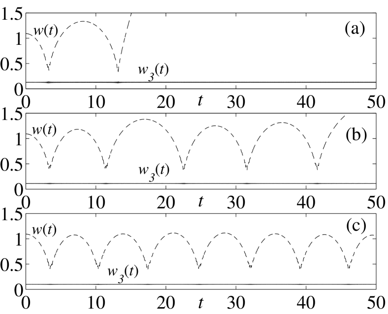
Figure 6: Stabilization of a Gaussian according to numerical simulations of Eq. (33) with parameters $g_{0}=(2\pi)^{1/2}(-2.2\pi)$, $g_{1}=(2\pi)^{1/2}8\pi$, $\Omega=40$, $w(0)=1.09$, $w_{3}(0)=w_{3,0}=\lambda_{3}^{-1/2}$. The evolution of the widths $w$ (dashed) and $w_{3}$ (solid) is shown for (a) $\lambda_{3}=60$, (b) $\lambda_{3}=80$ and (c) $\lambda_{3}=100$.

We have compared these results with the simulations of the full NLSE for the case when the potential is restricted to the $z$-axis and the system is strongly coin-shaped. To do so we have used a pseudo-spectral fully asymmetric 3D evolution method combined with a second order split-step method to advance in time. Typical grid sizes were of $128\times 128\times 64$.

In Fig. 7 we present the results for $g_{0}=(2\pi)^{1/2}(-2\pi)$, $g_{1}=(2\pi)^{1/2}8\pi$, $\Omega=40$, $\lambda_{3}=100$ and as initial data we take a Gaussian with $w(0)=1.09$ and $w_{3}(0)=\lambda_{3}^{-1/2}$. We see that, as in the two-dimensional case, part of the wave packet goes outside and after a readjustment the solution oscillates in the same way that in two dimensions. Moreover, the width $w_{3}$ remains nearly constant during the evolution.

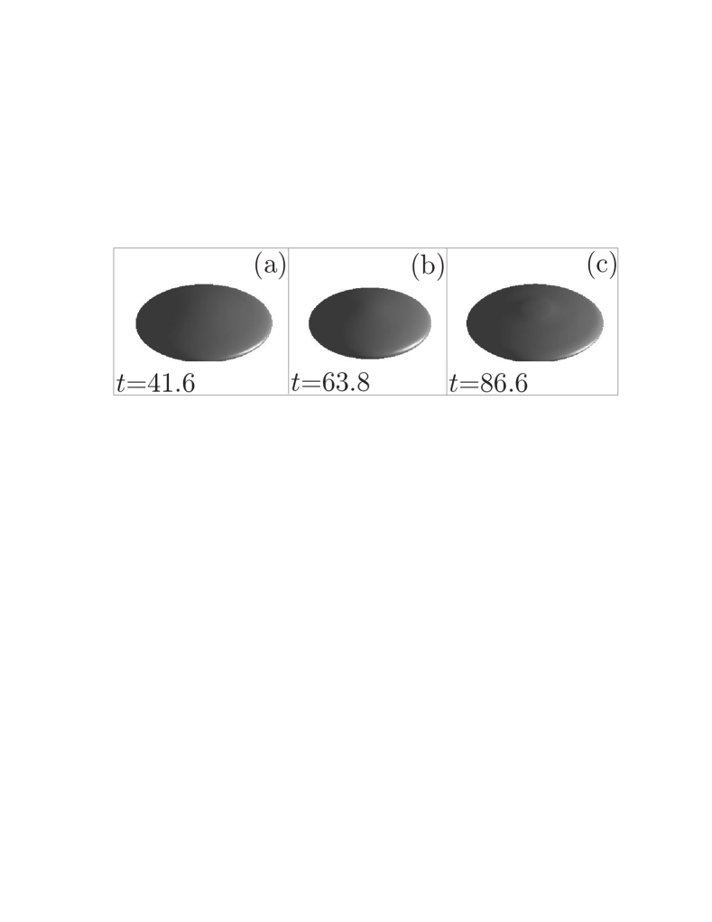
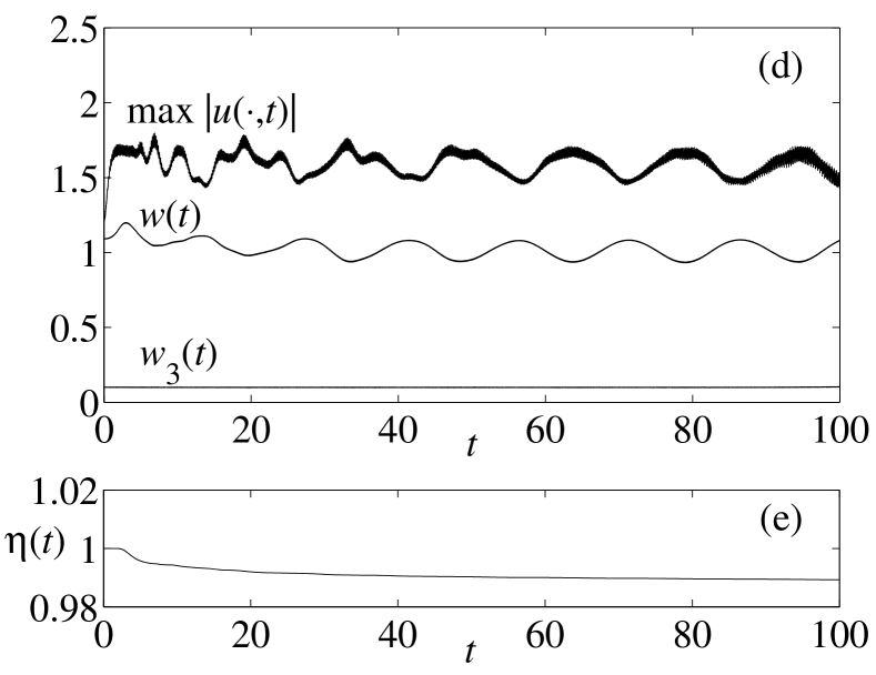
Figure 7: Results of numerical simulations of Eq. (2) showing stabilization of Gaussian initial data $\psi({\bf x},0)=(1/\pi^{3/4}w(0)w_{3}(0)^{1/2})e^{-(x^{2}+y^{2})/2w(0)^{2}}e^{-z^{2}/2w_{3}(0)^{2}}$ with widths $w(0)=1.09$ and $w_{3}(0)=\lambda_{3}^{-1/2}$ for parameter values $g_{0}=(2\pi)^{1/2}(-2\pi)$, $g_{1}=(2\pi)^{1/2}8\pi$, $\Omega=40$ and $\lambda_{3}=100$. (a-c) Isosurface plots of $|u({\bf x},t)|^{2}$ for $|u|^{2}=0.01$ corresponding to times of maximum (a,c) and minimum (b) width $w(t)$ of the solution. (d) Evolution of the widths $w(t)$ and $w_{3}(t)$ and of the amplitude $\max|u(\cdot,t)|$ of the solution. (e) Evolution of the norm $\eta(t)$.

6 Conclusions and discussion

In this paper we have provided a deeper understanding of the phenomenon of stabilization of solitons of the nonlinear Schrödinger equation by means of the control of the nonlinear term. We have developed the moment equations for 2D and 3D systems and obtained, on the basis of their rigorous analysis, precise conditions for the stabilization of 2D systems.

Taking as initial data Townes solitons or Gaussians for simulations based on Eq. (3) we have shown that the former is the structure which is stabilized and that other initial data which can be trapped must eject a fraction of the wave packet in the form of radiation to accomodate to this specific solution.

Also we have analyzed the three-dimensional situation. Here we have made an extensive search of stable regions according to our moment equations improving and extending the analysis of Ref. [21]. We have justified why moment-type equations cannot be used to predict the dynamics of the system. Only limited time stabilization is possible when the parameters are fine-tuned to very precise values. Finally, when a strong trapping along one specific direction is kept the system becomes effectively two-dimensional and it can be described again by variational methods whose predictions agree well with the full numerical simulations of the problem. In the latter case three-dimensional confinement is possible although there are only two spatial directions along which the solution is trapped by the nonlinear forces plus the stabilization mechanisms while the other direction is trapped by harmonic forces provided by the potential.

It is remarkable that the nonlinear Schrödinger equations support these stabilized structures which open new fields for applications, in fact these are the first stable structures obtained in the framework of the cubic nonlinear Schrödinger equation.

Many extensions of this work are possible. First, it would be very interesting to study the robustness of these breather-type solutions under different perturbations, e.g. by mutual collision of different structures in single and multicomponent systems. Secondly it could be interesting to try to stabilize other stationary structures different from the two-dimensional Townes soliton.

Acknowledgments

This work has been partially supported by the Ministerio de Ciencia y Tecnología under grants BFM2000-0521, BFM2002-01308 and Consejería de Ciencia y Tecnología de la Junta de Comunidades de Castilla-La Mancha under grant PAC02-002. G. D. Montesinos is supported by Ministerio de Educación, Cultura y Deporte under grant AP2001-0535.

References

- [1] L. Vázquez, L. Streit, V. M. Pérez-García, Eds. “Nonlinear Klein-Gordon and Schrödinger systems: Theory and Applications”, World Scientific, Singapore (1996).
- [2] C. Sulem and P. Sulem, “The nonlinear Schrödinger equation: Self-focusing and wave collapse”, Springer, Berlin (2000).
- [3] M. H. Anderson, J. R. Ensher, M. R. Matthews, C. E. Wieman, and E. A. Cornell, Science 269, 198 (1995).
- [4] K. B. Davis, M. O. Mewes, M. R. Andrews, N. J. Vandruten, D. S. Durfee, D. M. Kurn, and W. Ketterle, Phys. Rev. Lett. 75, 3969 (1995).
- [5] C. C. Bradley, C. A. Sackett, J. J. Tollett, and R. G. Hulet, Phys. Rev. Lett. 75, 1687 (1995).
- [6] C. C. Bradley, C. A. Sackett, and R. G. Hulet, Phys. Rev. Lett. 78, 985 (1997).
- [7] G. Baym and C. J. Pethick, Phys. Rev. Lett. 76, 6 (1996).
- [8] G. Fibich and G. Papanicolaou, SIAM J. Appl. Math. 60, 183 (1999).
- [9] C. A. Sackett, H. T. C. Stoof, and R. G. Hulet, Phys. Rev. Lett. 80, 2031 (1998).
- [10] C. A. Sackett, J. M. Gerton, M. Welling, and R. G. Hulet, Phys. Rev. Lett. 82, 876 (1999).
- [11] V. M. Pérez-García, H. Michinel, and H. Herrero, Phys. Rev. A, 57, 3837-3842 (1998).
- [12] V. M. Pérez-García, H. Michinel, J. I. Cirac, M. Lewenstein, and P. Zoller, Phys. Rev. A 56, 1424 (1997).
- [13] K. E. Strecker, G. B. Partridge, A. G. Truscott, and R. G. Hulet, Nature 417, 150-153 (2002).
- [14] L. Khaykovich, F. Schreck, G. Ferrari, T. Bourdel, J. Cubizolles, L. D. Carr, Y. Castin, and C. Salomon, Science 296, 1290-1293 (2002).
- [15] S. L. Cornish, N. R. Claussen, J. L. Roberts, E. A. Cornell, and C. E. Wieman, Phys. Rev. Lett. 85, 1795 (2000).
- [16] J. L. Roberts, N. R. Claussen, S. L. Cornish, E. A. Donley, E. A. Cornell, and C. E. Wieman, Phys. Rev. Lett. 86, 4211 (2001).
- [17] E. A. Donley, N. R. Claussen, S. L. Cornish, J. L. Roberts, E. A. Cornell, and C. E. Wieman, Nature 412, 295 (2001).
- [18] R. A. Duine and H. T. C. Stoof Phys. Rev. Lett. 86, 2204 (2001).
- [19] H. Saito and M. Ueda, Phys. Rev. A 65, 033624 (2002).
- [20] H. Saito and M. Ueda, Phys. Rev. Lett. 90, 040403 (2003).
- [21] F. Abdullaev, J. G. Caputo, R. A. Kraenkel, and B. A. Malomed, Phys. Rev. A 67, 013605 (2003).
- [22] F. Dalfovo, S. Giorgini, L. Pitaevski, and S. Stringari, Rev. Mod. Phys. 71, 463-512 (1999).
- [23] S. N. Vlasov, V. A. Petrischev, and V. I. Talanov, Radiophys. Quantum Electron. 14 (1971).
- [24] P. A. Belanger, Opt. Lett. 16 196 (1991).
- [25] M. A. Porras, J. Alda, and E. Bernabeu, Appl. Opt. 32 5885 (1993).
- [26] V. M. Pérez-García, M. A. Porras, and L. Vázquez, Phys. Lett. A 202 (1995) 176
- [27] J. J. García-Ripoll, V. M. Pérez-García, and P. Torres, Phys. Rev. Lett. 83, 1715-1718 (1999).
- [28] V. M. Pérez-García, G. D. Montesinos, J. J. García-Ripoll, and P. Torres, SIAM J. Sci. Comp. (submitted) (2003).
- [29] A. Görtlitz et al., Phys. Rev. Lett. 87 130402 (2001).
- [30] W. Paul, Rev. Mod. Phys. 62, 531-540 (1990).
- [31] C. King and A. Lesniewski, Lett. Math. Phys. 39, 367-378 (1997).
- [32] J. Lei and M. Zhang, Lett. Math. Phys. 60, 9-17 (2002).
- [33] I. Towers and B. Malomed, J. Opt. Soc. Am. B 19, 537 (2002).
- [34] R. Ortega, J. Diff. Eqns.128, 491-518 (1996).
- [35] C. L. Siegel and J. K. Moser, Lectures on Celestial Mechanics, Springer-Verlag, Berlin, 1971.
- [36] J. L. Massera, Duke Math. J. 17, 457 (1950).
- [37] S. Jiménez, I. M. Llorente, A. Mancho, V. M. Pérez-García, and L. Vázquez, Appl. Math. Comput. 134, 271 (2003).
- [38] T. R. Taha and M. Ablowitz, J. Comp. Phys. 55 (1984) 203.
- [39] S. Blanes and P. C. Moan, J. Comp. Appl. Math. 142, 313 (2002).
- [40] V. M. Pérez-García and X. Liu, Appl. Math. Comput., to appear.
- [41] M. Zhang and W. G. Li, Proc. Amer. Math. Soc. 130, 3325 (2002)