Basin bifurcations in a two-dimensional logistic map

Abstract

Previous works have been devoted to the study of two-dimensional noninvertible maps, obtained using a coupling between one-dimensional logistic maps. This paper is devoted to the study of a specific one, in order to complete previous results [6] [8], regarding the evolution of basins and attractors, when considering the tool of critical manifolds.

Mathematics Subject Classification 2000:  Primary 39B12, Secondary 26A18, 39B52. Keywords and phrases:  bifurcation, basin, logistic map, two-dimensional map, noninvertible, chaos.

1 Introduction

Many biological and physical phenomena are due to a complex connectivity among complex elements; feedback mechanism seems to be a suitable way to understand such phenomena (see for instance [3][4][5]). The introduction of feedback through a control parameter leads to models involving global multiplicative coupling among maps. One of the most simple models can be given by using logistic maps. Within this context, two-dimensional noninvertible maps with a global multiplicative coupling between one-dimensional logistic maps are of great interest. The understanding of their quite complex behaviour can be a first step in the understanding of dynamics in higher dimensional systems. Previous works (see [2][6][7][8]) have already been devoted to such kind of maps. In this paper, our aim is to complete the understanding of dynamics of model (c) given in [6].

The considered model is the noninvertible two-dimensional map $T$ defined by:

$$\left\{\begin{array}[]{cc}x_{k+1}=\lambda(3{y_{k}}+1)x_{k}(1-x_{k})\\ y_{k+1}=\lambda(3{x_{k+1}}+1)y_{k}(1-y_{k})\end{array}\right.$$ (3)

where $\lambda$ is a real control parameter, $x$ and $y$ are real state variables. The map  (3) includes a time asymmetric feedback. Numerical studies show that the system  (3) is stable when $\lambda\ \in[-1.5,1.19]$.

Section 2 is devoted to recalls about fixed points of the map (3) and their bifurcations. Section 3 concerns critical manifolds. Section 4 analyzes evolution of basins by considering crossing of basin boundary through critical curves. In section 5 we explain evolution of invariant closed curve issued from a fixed point and giving rise to $weakly\ chaotic\ ring\ (WCR)$, then to chaotic attractor.

2 Fixed points

As explained in [6], $T$ possesses at most five different fixed points :

$$P_{0}:x_{0}=0,\ y_{0}=0$$ (4)

$$P_{1}:x_{1}=\frac{\lambda-1}{\lambda},\ y_{1}=0,\quad P_{2}:x_{2}=0,\ y_{2}=\frac{\lambda-1}{\lambda}$$ (5)

$$P_{3}:x_{3}=\frac{1-\sqrt{a}}{3},\ y_{3}=\frac{1-\sqrt{a}}{3},\textrm{where }a=\frac{4\lambda-3}{\lambda},\ \lambda>\frac{3}{4}$$ (6)

$$P_{4}:x_{4}=\frac{1+\sqrt{a}}{3},\ y_{4}=\frac{1+\sqrt{a}}{3},\ \lambda>\frac{3}{4}$$ (7)

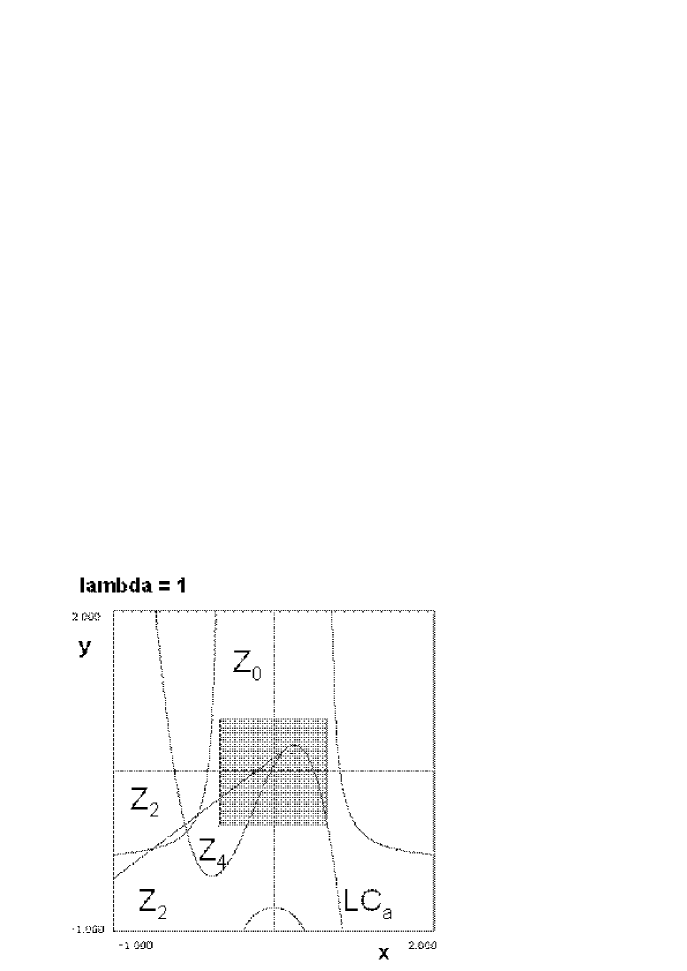
Figure 4: $\lambda$=1, the basin is a square.

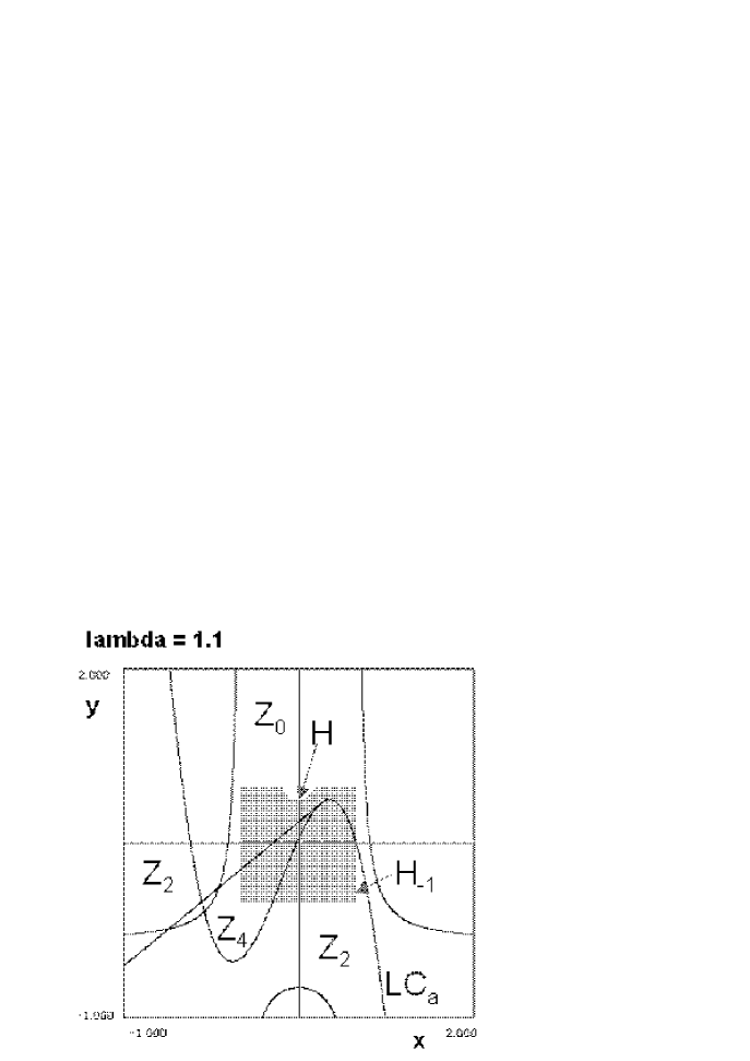
Figure 5: Creation of a bay H when $LC_{a}$ crosses through basin boundary; $\lambda$$\geq$1

.

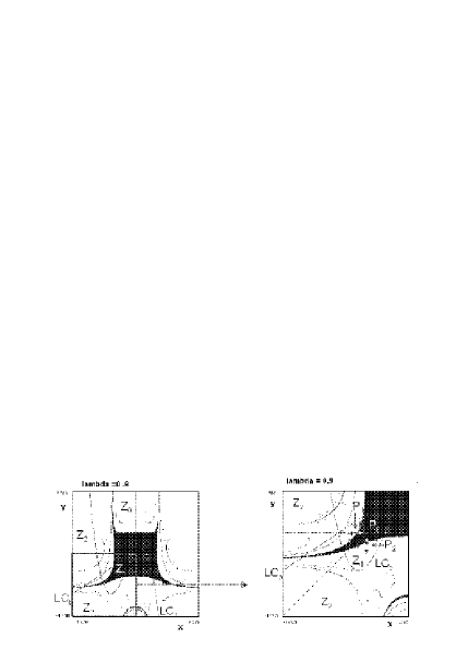
Figure 6: Creation of islands.

For $-1<\lambda<1$, $P_{0}$ is an attractive node and $P_{1}$ and $P_{2}$ are saddle points on the negative side of the axes, x–axis being $P_{1}$ unstable manifold and y–axis being $P_{2}$ unstable one. When $\lambda=1$, $P_{0}=P_{1}=P_{2}$. For $\lambda>1$, $P_{0}$ is a repulsive node and $P_{1}$ and $P_{2}$ are saddle points, but located on the positive side of the axes, which are now $P_{1}$ and $P_{2}$ stable manifolds (Figures 6–8). When $\lambda=-1$, $P_{0}$ undergoes a flip bifurcation and a period doubling cascade occurs when $\lambda$ decreases. $P_{3}$ and $P_{4}$ exist when $\lambda>\frac{3}{4}$. When $\lambda=\frac{3}{4}$, $P_{3}=P_{4}$; for $\frac{3}{4}<\lambda<1$, $P_{3}$ is a saddle point and $P_{4}$ an attractive node, the whole diagonal segment between $P_{3}$ and $P_{4}$ is locus of points belonging to heteroclinic trajectories connecting the two fixed points. When $\lambda=1$, $P_{4}$ undergoes a Neïmark–Hopf bifurcation and becomes repulsive by giving rise to an attractive invariant closed curve ($ICC$) ($C$). Section 5 is devoted to the study of ($C$) evolution.

3 Critical lines

An important tool used to study non-invertible maps is that of critical manifold, which has been introduced by Mira in 1964 (see [10][11] for more details). A non-invertible map is characterized by the fact that a point in the state space can possess different number of rank-1 preimages, depending where it is located in the state space. A critical curve LC, in the two-dimensional case, is the geometrical locus of points X in the state plane having two coincident preimages, $T^{-1}$(X), located on a curve $LC_{-1}$. It is recalled that the set of points $T^{-n}$(X) constitutes the rank–n preimages of a given point X. The curve LC verifies $T^{-1}$(LC)$\supseteq$$LC_{-1}$ or T($LC_{-1}$)=LC and separates the phase plane in two regions where each point has a different number of preimages (k in one region and k+2 in the other one, k $\in\mathbb{N}$). For the map  (3), $LC_{-1}$ is given by the cancellation of the Jacobian of the map.

For the map  (3), the critical manifold LC_-1 is given by four arcs (Figure 3):

$$LC_{-1a}:x=\frac{1}{2},\quad LC_{-1b}:y=\frac{1}{2},\quad LC_{-1d}:y=-\frac{1}{3}$$ (8)

$$LC_{-1c}:y=-\frac{1}{3}-\frac{1}{9\lambda x(1-x)}$$ (9)

and the critical manifold LC by (Figure 3):

$$LC_{a}:y=\frac{4\lambda}{9}(3x+1)(\frac{4x}{\lambda}-1)(1-\frac{x}{\lambda})$$ (10)

$$LC_{b}:y=\frac{\lambda}{4}(3x+1),x\leq\frac{5\lambda}{8}$$ (11)

$$LC_{c}=\left\{(x=-\frac{1}{3},y=0)\right\}\subset LC_{a}\cap LC_{b}$$ (12)

$$LC_{d}=\left\{(x=0,y=-\frac{4\lambda}{9})\right\}\subset LC_{a}$$ (13)

Let us call $Q_{c}$=$(x=\frac{5\lambda}{8},y=\frac{\lambda}{4}(\frac{15\lambda}{8}+1))$, $Q_{c}$ is a cusp point of $LC_{b}$, indeed $LC_{b}$ is constituted of two merged critical half straight lines ($x\ \in\ ]-\infty,\ \frac{5\lambda}{8}]$), which explains the fact that, by crossing $LC_{b}$, one goes from $Z_{4}$ area to $Z_{0}$ one, or from $Z_{2}$ to $Z_{2}$ (cf. Figure 3). Let us remark that $LC_{a}\cap LC_{b}=\left\{Q_{c},\ (x=-\frac{1}{3},y=0)\right\}$.

The LC curves separate the state space in different areas $Z_{i},\ i=0,2,4$ (Figure 3), where each point possesses $i$ distinct rank–1 preimages. Figure 3 shows the state space as a foliated one, each sheet corresponding to the existence of a rank–1 preimage. This foliation looks like those given for parameter plane, for instance in [9]. Previous representations of such foliation related to the existence of LC curves can be found in [13].

4 Evolution of basins

The basin of an attractor $B$ is defined as the set of all initial conditions that converge towards an attractor at finite distance when the number of iterations of $T$ tends towards infinity. The set $B$ verifies : $T^{-1}(B)=B$ and $T(B)\subseteq B$. We call $immediate\ basin$ the largest connected part of a basin containing the attracting set. In this section, we study the evolution of basin of attractors when parameter $\lambda$ is modified. The situations are shown in Figures 6 to 17. Using the terminology and the results of [10][11], our aim is to explain how basins become fractal, nonconnected or multiply connected in the case of  (3).

• Figure 6 shows the first modification of the basin with the creation of a $bay$ H, due to the crossing of $LC_{a}$ through the basin boundary. The $bay$ H is a rank–1 preimage of the area $H_{-1}$, which is located inside $Z_{2}$, when $\lambda$ increases from the value 1.

• The second modification consists in a bifurcation $connected\ basin\ \leftrightarrow\ nonconnected$ $basin$ when $\lambda$ decreases from the value 1. Islands are created (cf. Figures 6-8) after the bifurcation concerning the fixed points $P_{0},\ P_{1},\ P_{2}$. Indeed, when $\lambda$ decreases from the value 1, $P_{1}$ and $P_{2}$, located on positive part of axes, go to negative part of axes; the stable manifolds of these two saddle points is a part of the basin boundary; when the two points are on the negative part of axes, a tongue is created in the area ($x<0$, $y<0$) of the state space and crosses through $LC_{a}$ and $LC_{b}$ curves to penetrate inside $Z_{2}$ area, which is located above $LC_{b}$; it gives rise to a sequence of infinitely many preimages of any rank of this part of the tongue: these are the islands, the basin becomes non connected.

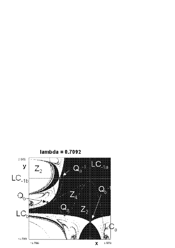
Figure 10: Enlargment of Figure 10.

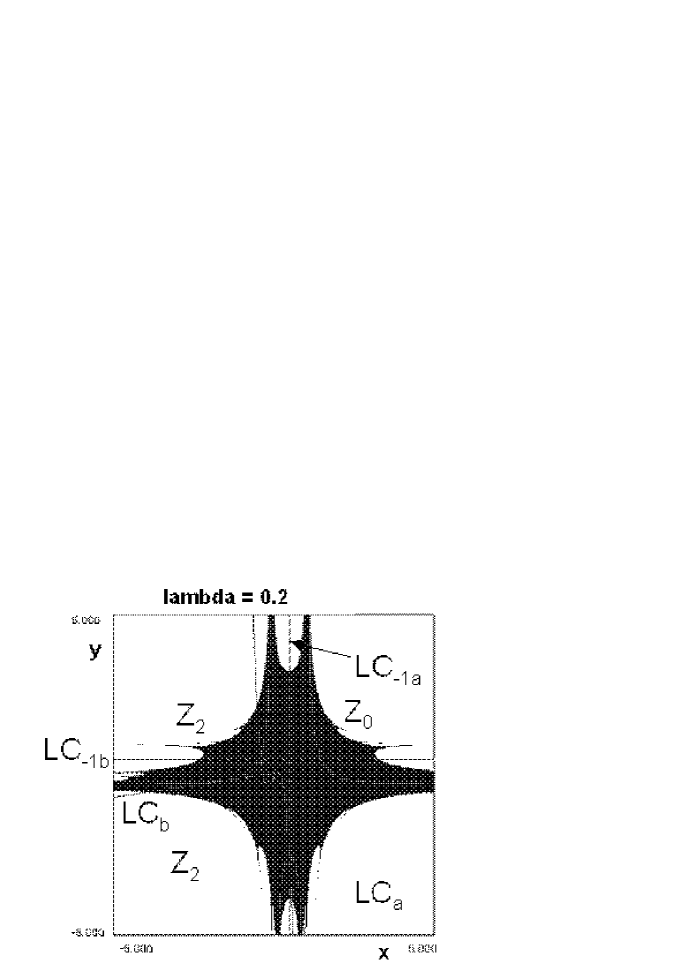
Figure 12: Tongues disappear by crossing of basin boundary through critical curves.

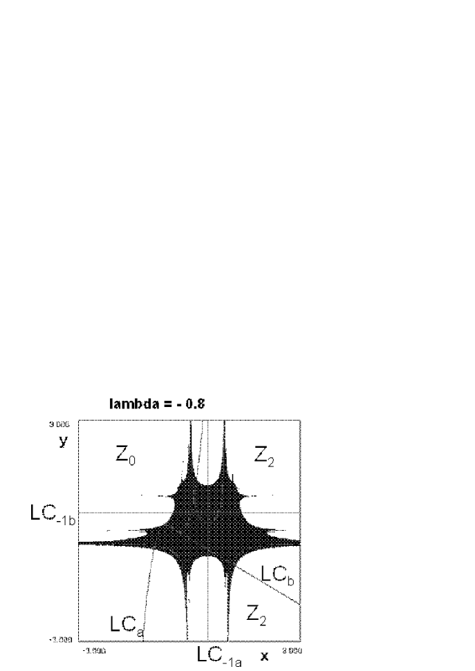
Figure 14: Tongues appear again when $\lambda$$<$0.

• The third modification of the basin is due to a sequence of $aggregations\ of\ islands$ (Figures 8-12). The first aggregation occurs when $LC_{a}$ and $LC_{b}$ curves become tangent in points $Q_{a}$ and $Q_{b}$ at the basin boundary (Figure 10), rank–1 preimages of $Q_{a}$ and $Q_{b}$, $Q_{a}^{-1}$ and $Q_{b}^{-1}$, correspond to the aggregation of two islands with the immediate basin. The other preimages of $Q_{a}$ and $Q_{b}$ give rise to other aggregations. This first aggregation is followed by infinitely many new aggregations due to tangencies between critical curves and the immediate basin boundary when $\lambda$ decreases; such phenomena are explained more precisely in [12]. The important point to note is that a crossing between critical curves and basin boundary makes some domains change $Z_{i}$ area, so it makes appear or disappear preimages of the considered domains. The sequence of aggregations is nearly finished in Figure 12. The basin size increases when the parameter $\lambda$ decreases and tongues corresponding to island ends disappear when crossing critical curves of different rank (Figure 12). In Figure 14, the basin boundary is smooth. When $\lambda$ decreases, being negative, an inverse process gives rise to new appearance of tongues (Figure 14).

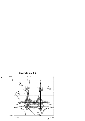
Figure 17: Basin boundary is fractal. An attractive period–2 cycle exists.

• Another modification corresponds to a bifurcation $connected\ basin$ $\leftrightarrow$ $multiply-connected\ basin$, that means basin with holes inside. The appearance of these holes is also related to crossing of basin boundary through critical curves; for instance, the hole in the middle of the basin in Figure 16 is due to the crossing of $LC_{a}$ near its left extremum; it makes appear an area in $Z_{2}$ region and the preimages of any rank of this area gives rise to infinitely many holes inside the basin; these holes accumulate along the basin boundary. When $\lambda$ decreases, the size of holes increases (Figure 16). Some holes can open and be changed in $bays$ (cf. [10][11]), this is the case in Figure 17, the basin boundary becomes fractal.

5 Evolution of attractors

This section is devoted to the study of evolution of attractors when $\lambda$ increases. This evolution can involve relations with the attractor basin or homoclinic and heteroclinic bifurcations.

• When $\lambda$= 1, the attractive focus undergoes a Neïmark–Hopf bifurcation and becomes repulsive when giving rise to an attractive $ICC$ $(C)$ (Figure 21). Oscillations appear on $(C)$ when it is tangent to the cusp point $Q_{c}$ on $LC_{b}$ (Figure 21). From $\lambda=1.11$, $\lambda$ increasing, there is an alternation between existence of $ICC$ with oscillations, frequency lockings, cyclic chaotic behaviors, contact bifurcations with basin boundaries and single chaotic attractor. These results are consistent with the Liapunov exponents values obtained in [6]. We are going to explain what occurs regarding contact with basins of coexisting period–3 attractors.

• In the same time, two attractive period–3 orbits appear simultaneously by a fold bifurcation, coexisting with two period–3 orbits of saddle points (Figure 21). So, three different attractors coexist; Figure 21 shows the basin of the $ICC$ and the basin of the two period–3 attractors. When $\lambda$ increases, the two period–3 attractive cycles undergo a Neïmark–Hopf bifurcation and become unstable by giving rise to two period–3 attractive $ICC$ around them. Figure 21 shows the three different basins of the three coexisting attractors : in this case, two period–3 $ICC$ and a period–29 attractive cycle, which corresponds to a frequency locking for the $ICC$.

• When $\lambda$ increases, the $ICC$ appears again; curles arise, due to crossings of $(C)$ through critical curves, and involve auto–intersections of $(C)$, the $ICC$ is then called a $weakly\ chaotic\ ring\ (WCR)$ [11] (Figure 24). The existence of curles changes the shape of the $ICC$ and generates contact with its basin boundary; this implies the explosion of $(C)$ and makes it disappear. Then, the basin of the former $ICC$ becomes part of the basin of the other attractors (Figures 24 $\&$ 28).

• Figure 24 shows the separate basins of each part of the two period–3 attractive $ICC$, that means basins for $T^{3}$ are plotted.

• Another contact bifurcation occurs, which involves the manifolds of the period–3 saddle cycles, born by fold bifurcation. This contact creates a new attractor, by mixing the two former period–3 $ICC$ (Figure 28). This new attractor evolves, undergoes frequency lockings, which give rise to the appearance of cyclic chaotic attractor (Figure 28); curles appear on the attractor and it becomes a $WCR$ (Figures 28–32), then it becomes a chaotic attractor; chaos becomes stronger and stronger (Figures 32–34).

• The chaotic attractor disappears when a contact bifurcation occurs between the attractor and its basin boundary (Figure 34).

6 Conclusion

Complex behaviour of a two-dimensional noninvertible map with a multiplicative global coupling between one-dimensional logistic maps, including a time asymmetric feedback, has been analyzed. The different kinds of basin bifurcations which occur when the parameter is modified and the evolution of attractors issued from Neïmark–Hopf bifurcation have been explained. The fundamental point, as previously obtained in two-dimensional noninvertible maps studies, is the position of basins and attractors, regarding critical curves. $Islands\ aggregations$, $connected\ basin\ \leftrightarrow\ nonconnected$ $basin$, $connected\ basin$ $\leftrightarrow$ $multiply-connected\ basin$, change of $Invariant\ Closed\ Curve$ into $Weakly\ Chaotic\ Ring$ or $Strong\ Chaotic\ Attractor$ are bifurcations in relation with critical curves.

7 Acknowledgment

We would like to thank Prof. Mira for helpful discussions, in particular, the Figure 3 is due to him. R. Lopez-Ruiz wishes to thank the Program Europa of CAI–CONSI+D (Zaragoza, Spain) for financial support.

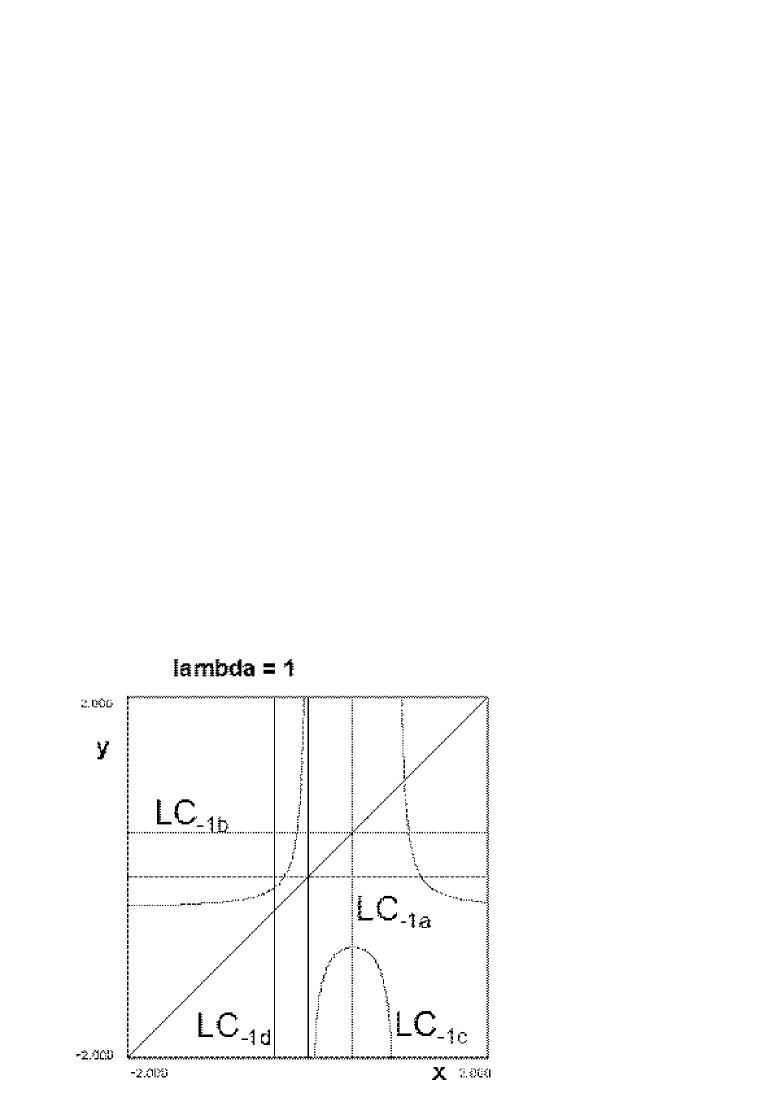
Figure 1: Preimages of critical lines:
$LC_{-}$₁ arcs.

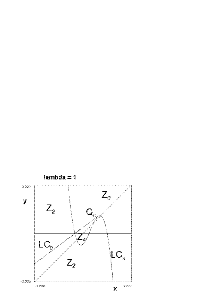
Figure 2: Critical lines LC and $Z_{i}$ areas in the state plane.

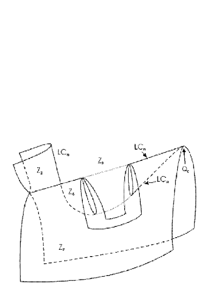
Figure 3: Qualitative representation of the foliation of the state space, the open U-shaped window permits to show a section of $Z_{4}$ and $Z_{2}$ area. On the right end, one can see the cusp point $Q_{c}$ on $LC_{b}$.

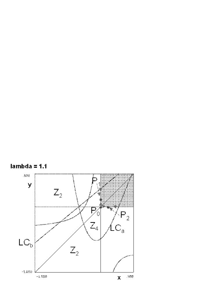
Figure 7: Before the bifurcation
connected basin $\leftrightarrow$ nonconnected basin.

Figure 8: Before islands aggregation.

Figure 9: Islands aggregation.

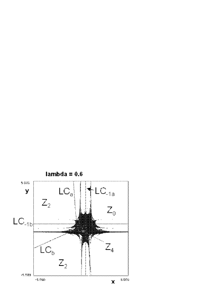
Figure 11: A sequence of islands
aggregations occurs when $\lambda$ decreases.

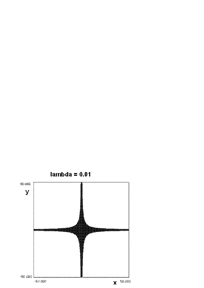
Figure 13: The basin boundary is smooth.

Figure 15: Basin becomes multiply
connected.

Figure 16: When $\lambda$ decreases, the size of holes increases. $P_{0}$ has undergone a flip bifurcation: an attractive period–2 cycle exists.

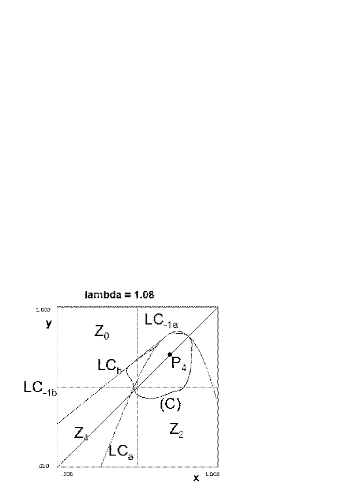
Figure 18: An attractive invariant closed
curve $(C)$ exists around the fixed point $P_{4}$.

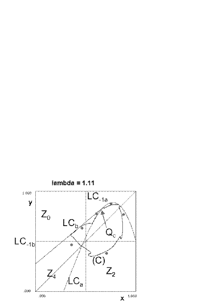
Figure 19: Two stable 3-periodic orbits appear by fold bifurcation; oscillations appear on $(C)$ when it is tangent to the cusp point $Q_{c}$ on $LC_{b}$.

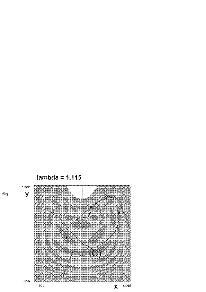
Figure 20: Basins of the $ICC$ and of the
two period–3 attractive cycles.

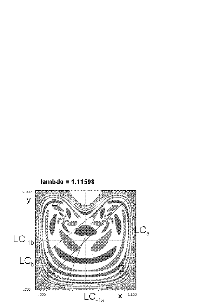
Figure 21: Frequency locking on a period–29 cycle for the $ICC$ and Neïmark–Hopf bifurcation for the two period–3 attractive cycles.

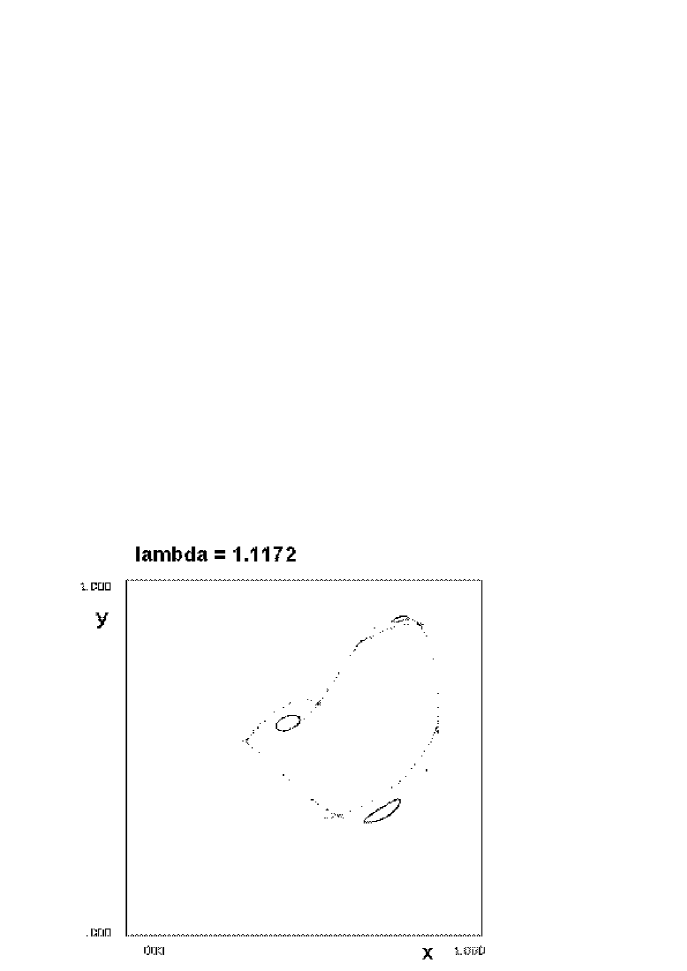
Figure 22: Transient after that the $ICC$
$(C)$ has disappeared, the initial condition
(.5,.51) gives rise to a trajectory, which
follows the shape of the former $ICC$ $(C)$,
before reaching one of the period–3 $ICC$.

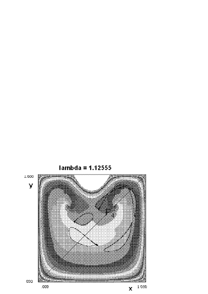
Figure 23: Basins for the map T³. It permits to see the basin of each curve, part of period–3 $ICC$.

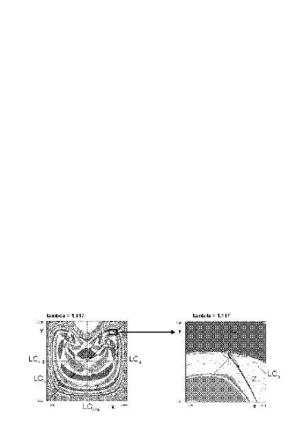
Figure 24: The curve $(C)$ becomes a $weakly\ chaotic\ ring$ when curles arise on it.

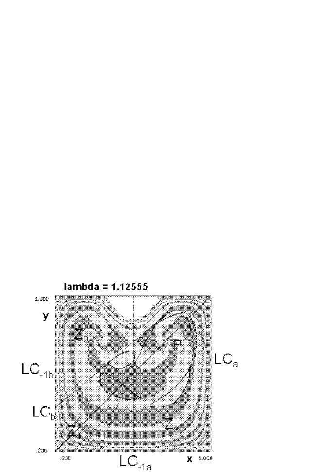
Figure 25: Two 3–periodic stable $ICC$
and their basin.

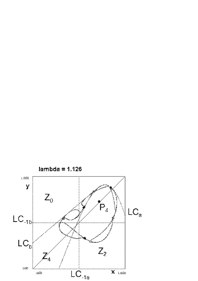
Figure 26: After contact bifurcation, a single attractor exists.

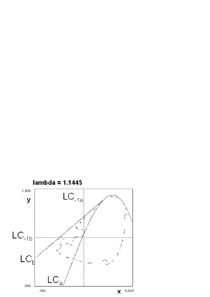
Figure 27: Cyclic chaotic attractor.

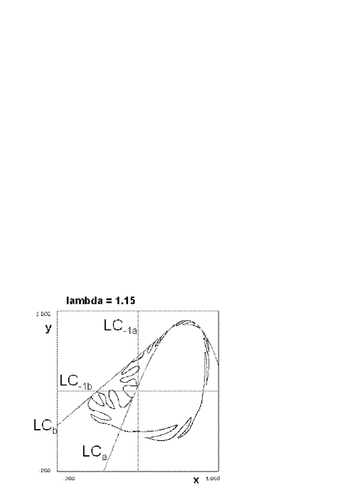
Figure 28: Oscillations increase.

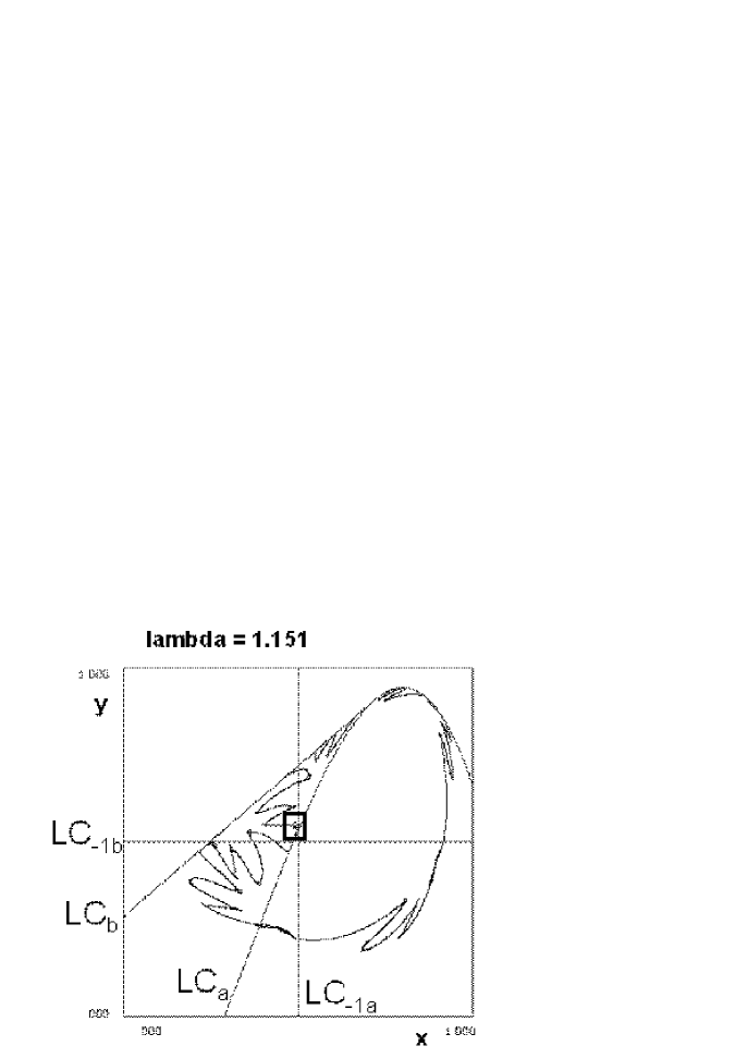
Figure 29: Curles issued from heteroclinic tangencies.

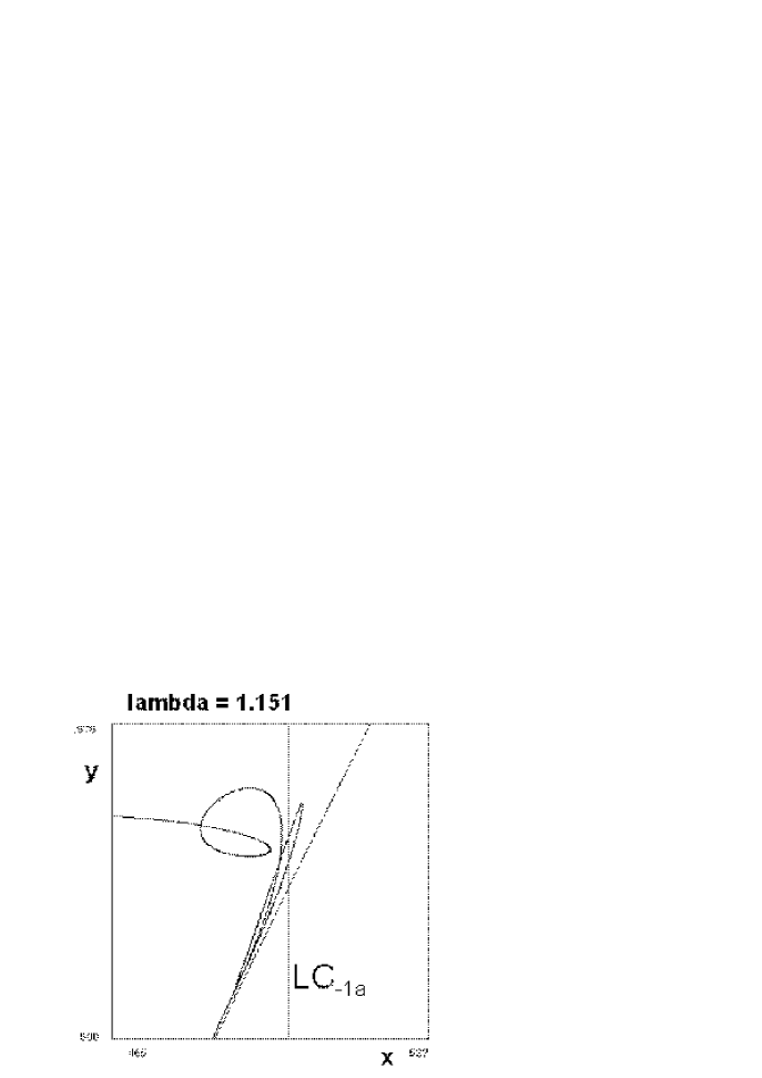
Figure 30: Enlargment of Figure 32

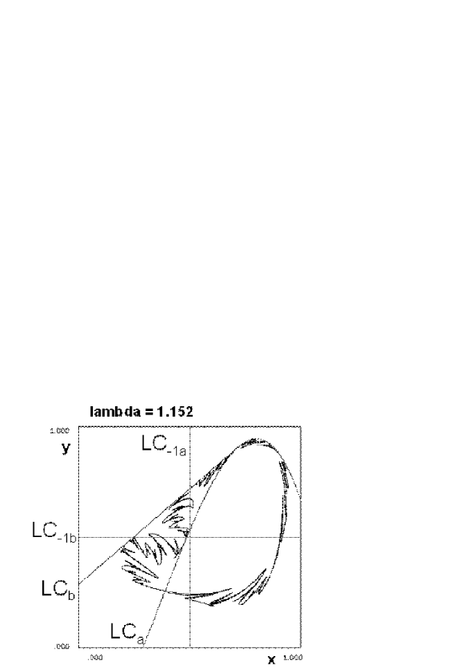
Figure 31: Oscillations increase on the $WCR$.

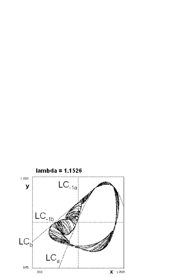
Figure 32: Chaotic attractor.

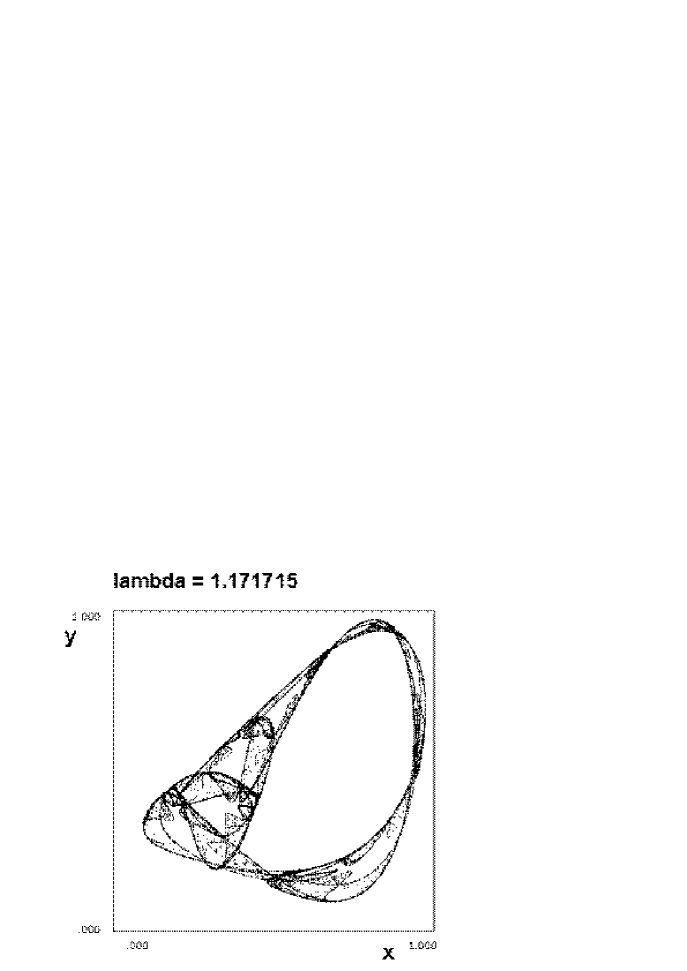
Figure 33: Chaotic attractor.

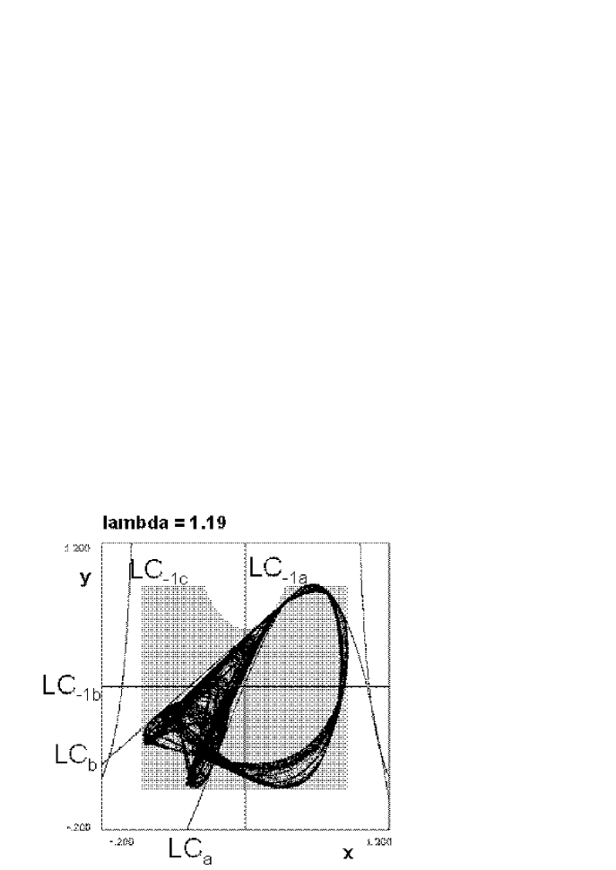
Figure 34: Contact bifurcation of the chaotic attractor with its basin boundary.

References

- [1]
- [2] Gardini, L., Abraham R., Fournier-Prunaret, D., Record, R., A double logistic map, Int. J. Bif. Chaos, vol. 4, 1 (1994), 145–176.
- [3] Kaneko, K., Chaotic but regular posi-nega switch among coded attractors by cluster–size variation, Phys. Rev. Lett., 63,(1989), 219–223.
- [4] Kaneko, K., Spatiotemporal chaos in one-dimensional and two-dimensional coupled lattices, Physica D, 37, (1989), 60–84.
- [5] Kaneko, K., Clustering, coding, Switching, hierarchical ordering and control in network of chaotic elements, Physica D, 41, (1990), 137–172.
- [6] Lopez-Ruiz, R., Perez-Garcia, C., Dynamics of maps with a global multiplicative coupling, Chaos, Solitons and Fractals, vol.1, 6 (1991), 511–528.
- [7] Lopez-Ruiz, R., Perez-Garcia, C., Dynamics of two logistic maps with a global multiplicative coupling, Int. J. Bif. Chaos, vol. 2, 2 (1992), 421–425.
- [8] Lopez-Ruiz, R., Fournier-Prunaret, D., Complex patterns on the plane : different types of basin fractalizations in a 2-D mapping,Int. J. Bif. Chaos, vol.13, 2 (2003), 281–310.
- [9] Mira, C.,,Chaotic Dynamics. From the one-dimensional endomorphism to the two-dimensional diffeomorphism, World Scientific Publishing, Singapore,(1987).
- [10] Mira, C., Fournier-Prunaret, D., Gardini, L., Kawakami, H., Cathala, J.C., Basin bifurcations of two-dimensional noninvertible maps. Fractalization of basins, Int. J. Bif. Chaos, vol. 4, 2 (1994), 343–381.
- [11] Mira, C.,Gardini, L., Barugola, A., Cathala, J.C.,Chaotic Dynamics in Two-Dimensional Noninvertible Maps, World Scientific Publishing, Singapore, series A, vol. 4,(1996).
- [12] Mira, C., Rauzy, C., Fractal aggregation of basin islands in two-dimensional quadratic noninvertible maps, Int. J. Bif. Chaos, vol. 5, 4 (1994), 991–1019.
- [13] Mira, C., Carcasses, J.P., Millerioux, G., Gardini, L. Plane foliation of two-dimensional noninvertible maps. Fractalization of basins, Int. J. Bif. Chaos, vol. 6, 8 (1996), 1439–1462.